How VMI Can Be Successful in Gas Distribution
A Solution Methodology for the Inventory Routing Problem
in Gas Distribution
P.J.H. Hulshof, MSc
August, 2008, University of Twente
Committee E.W. Hans, PhD, MSc
A.L. Kok, MSc A. Hoendervoogt, MSc J. Meesters, MSc
How VMI Can Be Successful in Gas Distribution, Peter Hulshof 2
Preface
I have experienced my student time as a marvellous time, studying, travelling, starting a company, participating in student organisations, and meeting many different people and cultures. I thank all my friends and family for this wonderful experience.
Graduation is a rough experience to many people, but I experienced it as an interesting period full of exploration as well. This was mainly because ORTEC provided me with an interesting project and all the support that I needed. ORTEC made it possible that I could visit two planning sites in the Netherlands and in the United Kingdom to learn more about the practice of gas distribution. I thank ORTEC for offering me this research project, and I especially thank Arjan Hoendervoogt en Janneke Meesters for their support. Additionally, I thank the complete department of ORTEC Oil, Gas and Chemicals, who I bothered with many questions, and Joaquim Gromicho and Goos Kant from ORTEC for the meetings we had about the algorithm design.
Next to ORTEC, I was also motivated by the enthusiasm of Erwin Hans and Leendert Kok, my supervisors at the University of Twente. I thank them for their unbiased views and challenging propositions that always kept me thinking. Additionally, I thank Professor Dror from the University of Arizona for sending me his articles by mail.
Graduation is not always a sweet journey, and I thank my girlfriend, Kirsten, and my roommate, Jesse, for helping me through the tougher periods.
It is very sad that my grandfather passed away three months before my graduation, he would have been as proud as the rest of my family is now. He inspired, and always will inspire me to study more and to reach for higher objectives. I thank my father, Jacques, my mother, Ineke, my sister, Annelies, and the rest of my family for all their support during my studies, and for teaching me more than I will ever learn somewhere else.
Peter Hulshof
How VMI Can Be Successful in Gas Distribution, Peter Hulshof 3
Abstract
This research is done at the department Oil, Gas, and Chemicals at ORTEC, a planning software company. We study the distribution of gas to commercial and residential customers that are not connected to a network of gas pipelines. These customers receive gas deliveries under a Vendor Managed Inventory (VMI) contract, which gives gas companies the flexibility to determine when and what volume to deliver, and what routes to choose. The decision problem that is associated with VMI for a large set of customers is the Inventory Routing Problem (IRP). Additionally, gas companies want to control the effects of the large seasonal peak in gas demand, to use the available resources efficiently. This research assumes customer usage to be deterministic, and we develop a solution for a region with multiple depots and vehicles with varying capacity (heterogeneous fleet). Introduction
To design a solution methodology to minimize distribution costs in the IRP for gas distribution, and mitigate the seasonal peak in customer deliveries.
We propose a solution methodology that increases the volume per kilometre, since it is an important indicator of distribution costs. Additionally, we balance the delivery volume in the planning period, to use the available resources efficiently. To mitigate the seasonal peak, we balance the delivery volume over a relatively long period, so that the workload is more equally divided over the year.
Objective
An algorithm is developed to select a certain delivery day in the planning period for every customer. The algorithm focuses on finding delivery days for customers that can receive a relatively large delivery compared to the customer’s capacity, while minimizing total travel distance. Customers that require a delivery in the planning period must be planned, and the customers that do not require a delivery in the planning period are planned according to the impact of the delivery on total travel distance and on future planning periods. The delivery volume is balanced according to the available vehicle capacity to efficiently use the available workforce and to smoothen the delivery volume over the course of a year.
Solution
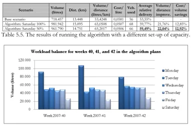
Actual delivery data from a large gas company are used to test the algorithm in a planning period of seven days. The computational experiments show that the solution increases the delivered volume per kilometre by more than 21%. The delivery volume is balanced on the short-term and long-term, and is responsive to changes in the vehicle capacity in the planning period.
Results
The solution decreases the costs for gas distribution, and requires an acceptable computation time. The long-term balance in delivery volume flattens the customer delivery curve, and thus helps in mitigating the seasonal peak.
How VMI Can Be Successful in Gas Distribution, Peter Hulshof 4
Contents
Preface ... 2
Abstract ... 3
Definitions ... 6
1 Introduction ... 7
1.1 Thesis structure ... 7
1.2 ORTEC ... 7
1.3 Problem description ... 8
1.4 Objective ... 9
1.5 Scope ...10
1.6 Research questions ...10
2 Context analysis ... 11
2.1 The Inventory Routing Problem ...11
2.1.1 The IRP in an example ...12
2.2 Gas distribution ...13
2.2.1 The economics of gas distribution ...14
2.2.2 Solution requirements for gas distribution ...15
2.3 ORION and SHORTREC ...15
2.4 The background solution: Period Scheduler ...16
2.4.1 Background solution analysis ...17
2.5 Solution requirements ...17
3 Literature analysis ... 18
3.1 Key principles in solving the IRP ...18
3.2 Solution methodology for the IRP ...19
3.3 Performance measurement for the IRP ...21
3.4 Seasonal peak problem ...21
3.5 Decision models to optimize the IRP solution ...22
3.5.1 Integer Linear Programming ...22
3.5.2 Mixed Integer Linear Programming ...23
3.5.3 Dynamic Programming ...23
3.6 Main conclusions from the literature ...23
4 Solution ... 24
4.1 Algorithm design ...24
4.1.1 Solution requirements...24
4.1.2 Assumptions ...24
4.2 Algorithm description ...25
4.2.1 Algorithm overview ...25
4.2.2 The algorithm in detail ...26
4.2.2.1Step 1: Customer selection ...26
4.2.2.2Step 2: Flexible clustering ...27
4.2.2.3Step 3: Generation of schedules ...28
4.2.2.4Step 4: Schedule assignment with an ILP for seed customers ...29
4.2.2.5Step 5: Schedule assignment with an ILP for clustered customers ...31
4.3 Alternative algorithm designs ...34
4.4 Distance types ...35
How VMI Can Be Successful in Gas Distribution, Peter Hulshof 5
5 Computational results ... 36
5.1 Experimental design ...36
5.1.1 Algorithm settings ...36
5.1.2 Dataset ...36
5.1.3 Assumptions ...38
5.2 Comparison base scenario and algorithm ...38
5.2.1 Weekly comparison ...38
5.2.2 Workload balance ...39
5.2.3 Different vehicle capacity set-up ...41
5.3 Sensitivity analysis ...42
5.3.1 Setting αin customer selection ...42
5.3.2 Long-term workload balance ...44
5.3.3 Short-term workload balance ...45
5.3.4 Distance types ...45
5.4 Testing alternative algorithm designs ...46
6 Conclusions and recommendations ... 47
6.1 Conclusions ...47
6.2 Recommendations ...48
6.2.1 Long-term recommendations ...48
6.2.2 Short-term recommendation ...48
6.3 Scientific contributions ...48
6.4 Future research ...49
References ... 50
Appendices ... 52
Appendix A: The Period Scheduler: Seed selection procedure ...53
Appendix B: The Period Scheduler: ILP model ...54
Appendix C: Extended literature summary ...55
C.1 Key principles in solving the IRP ...55
C.2 Solution methodology for the IRP ...57
C.3 Performance measurement for the IRP ...63
C.4 Seasonal peak problem ...64
Appendix D: Forecasted and actual customer usage curves ...65
Appendix E: Symbols used in the mathematical formulations ...68
Appendix F: Workload calculation: Step 4 ...70
Appendix G: Workload calculation: Step 5 ...72
Appendix H: Workload calculation: Improving the balance ...75
Appendix I: Alternative designs: Balance customers ...76
Appendix J: Alternative designs: Different objective functions ...80
Appendix K: Alternative designs: ILP with combination check ...82
Appendix L: Settings used in the computational tests ...83
Appendix M: Dataset overview ...84
Appendix N: Comparison actual routes and SHORTREC routes ...85
Appendix O: Computational results: The weekly comparison ...86
Appendix P: Computational results: The working time balance ...87
Appendix Q: Computational results: A different vehicle set-up ...88
Appendix R: Computational results: α parameter ...89
Appendix S: Computational results: Bandwidth parameter ...90
Appendix T: Computational results: Distance type parameter ...91
How VMI Can Be Successful in Gas Distribution, Peter Hulshof 6
Definitions
This research is about propane gas, and we refer to propane gas simply with gas. Propane gas is used for heating residential and company buildings.
An order is an intention to buy or sell a certain amount of goods. An order can be
pulled, meaning that an order is an instruction from the buyer that he wants to buy. If an order is pushed, an order is forecasted by the seller, and delivered to the buyer. A
delivery is a planned and scheduled order, waiting to be delivered, and an actual delivery is a completed delivery.
Volatility is the standard deviation in demand. A volatile good refers to a good that has a relatively unstable demand curve with many peaks. The safety stock is a certain amount of stock that is kept to buffer against stock outs. In a highly volatile market, safety stock should be chosen to be relatively high, because peaks in demand are larger, and thus the risk of a stock out is larger (Brown et al., 2002). A seasonal profile reflects the volatility of a good in a year, for instance an increase in demand in the winter period.
Workload balancing has the objective to balance the volume of work over periods of time, to have a relatively constant flow of work, and to mitigate the influence of volatility.
A client is a customer of ORTEC. In this thesis the gas companies are clients. A
customer needs to be replenished by ORTEC’s client. A location is a customer that needs to be visited in the routing problem.
A ‘must-go’ customer requires a delivery in the planning period, because the customer will reach safety stock otherwise. A ‘may-go’ customer will not reach safety stock in the planning period, but may be delivered to create efficient routes.
The visit frequency is the number of visits per period that are needed to replenish a certain customer. Slow-movers are customers that have a relatively low visit frequency, for instance once per year. Fast-movers have a relatively high visit frequency, for instance once per week.
A truck is a lorry without a trailer. The trailer is a compartment to store and transport goods in. In our thesis, the trailer is a large tank, which is pulled by a truck. A driver is an employee that drives the truck to its destination. A vehicle is a combination of a truck, a trailer, and a driver. Vehicle capacity may vary, and a certain vehicle type indicates a vehicle with a certain load capacity.
A depot is a central location in a region with a large stock of gas, and where vehicles can load and unload. In this thesis, it is assumed that depots have infinite stock.
A trip is a set of orders that can be delivered by a vehicle in one haul, with the restrictions on the driver’s work time and the vehicle’s capacity taken into account. A vehicle can perform multiple trips per day.
How VMI Can Be Successful in Gas Distribution, Peter Hulshof 7
1
Introduction
Gas is a commodity, which is of crucial importance to our daily lives. Gas is used for heating our houses or work environment. To deliver gas to their customers, gas companies make a complex set of decisions in exploration, production, and distribution. Although most customers are connected to large national networks of pipelines, some customers are not. For these customers, gas is supplied by trucks and stored in large tanks at the customer’s location. To make transportation by truck more efficient, gas companies supply gas to their customers according to a Vendor Managed Inventory (VMI) agreement. With VMI, the decision to deliver gas lies with the gas company, and not with the individual customer.
When a customer agrees with a VMI contract, a gas company can choose how often, when, and in what quantities the customer is replenished. In return, the gas company ensures that the customer will never run out of stock. In order to do this, a gas company needs to forecast and monitor the customer’s gas usage. This gas usage is influenced by the outside temperature, meaning that usage rises when temperature is low and vice versa. Due to this dependence, there is a high peak in gas demand in the winter months. This increases pressure on the gas company’s resources, and eventually leads to stock outs at customers in periods of high demand.
This research proposes a solution methodology to find a better distribution strategy when a gas company has the freedom that comes with VMI, and to mitigate the delivery peak in the winter months. The structure and lay-out of the thesis is discussed in Paragraph 1.1. This research has been done at ORTEC; we discuss the company in Paragraph 1.2. Paragraph 1.3 describes the problem, and Paragraph 1.4 states the research objective. The scope of the project is discussed in Paragraph 1.5, and Paragraph 1.6 clarifies the research questions.
1.1 Thesis structure
• Chapter 1 states an overview of the research. The company ORTEC is described, and we give a description of the problem.
• In Chapter 2, we analyze the context of the problem. We discuss the main problem, gas distribution, the involved software suites, and the background solution currently in place.
• Chapter 3 describes the literature that applies to the research questions in this thesis.
• Chapter 4 describes our solution, based on the information from Chapters 2 and 3.
• In Chapter 5, we discuss the computational results and a sensitivity analysis.
• In Chapter 6, we discuss the conclusions and the recommendations. We also discuss the scientific contributions of our report, and state ideas for future research.
1.2 ORTEC
How VMI Can Be Successful in Gas Distribution, Peter Hulshof 8
1.3 Problem description
Gas companies supply gas to their customers according to a VMI agreement. The gas company can optimize its decisions on the condition that at least a minimum stock of gas is always available to the customer. This minimum stock is called the safety stock, and it serves as a buffer to prevent stock outs. Because of VMI, gas companies forecast the customer usage, and have more freedom in creating their distribution plan. Additionally, customers do not need to dedicate resources to inventory management.
ORTEC provides a software solution called ORION to support gas companies in forecasting gas usage with historical delivery data. From the forecasted usage, orders are generated which are exported to SHORTREC, a software product that creates solutions for large instances of the Vehicle Routing Problem (VRP). The VRP is the problem of selecting a set of routes for a certain vehicle fleet in such a way that all orders are delivered at minimal costs (Dantzig and Ramser, 1959).
Figure 1.1. The two distinct phases in planning and scheduling of all customer deliveries.
ORION and SHORTREC decompose the problem of planning and scheduling into two clear phases that are illustrated in Figure 1.1.
ORION plans the delivery date of an order with an algorithm that minimizes the number of visits. This means a customer is served as late as possible, just before the customer reaches safety stock. According to Campbell and Savelsbergh (2004), this approach maximizes the volume deliverable to a customer, but may not create an optimal solution on the long-term, since it does not recognize geographical synergies between customers. The savings in synergy may be higher than the savings in minimizing the number of visits, for instance if two customers are located not far from each other, but should be visited on a different day according to ORION. Figure 1.2 illustrates this problem.
ORION plan for day one ORION plan for day two
depot depot
Figure 1.2. The blue arrow indicates that the order (in red) is more efficiently delivered, when it is delivered on the same day as customers in close vicinity.
Phase 1 - Planning
Generating orders in ORION
Phase 2 - Scheduling
How VMI Can Be Successful in Gas Distribution, Peter Hulshof 9 Figure 1.3. The actual weekly delivery volumes of gas in the Northern-England region
(NE-region) clearly show the seasonal peak in demand in the winter months
Figure 1.3 illustrates a large and long lasting peak in the demand for gas in the winter months; all other peaks and disturbances are explained in Paragraph 2.2. On average, the volume delivered to customers in the winter months is 1,5 times as high as the amount delivered in the summer months. The workload balance over a full year is offset by the large peak in demand in the winter months. This leads to stock outs at customers during the winter months and, in combination with a fixed fleet over the year, to unused trucks in the summer months. If we want to balance the workload over a full year, it is important to consider the expected demand in a longer period in the short-term plan. Currently, there is no available method in ORION or SHORTREC to plan and schedule orders, taking future total demand in the region into account.
Additionally, we study the problem of unstable workload balance on the short-term. To explain this problem, we provide an example: if fewer orders are planned on Wednesday than on Friday, we do not need all trucks on Wednesday. Then on Saturday, we need an emergency truck, since not all orders can be delivered on Friday, and this results in high costs.
In the literature, the problem described in this paragraph is referred to as an Inventory Routing Problem (IRP). The IRP is similar to a VRP with two additional questions: (1) when to serve a customer, and (2) how much to deliver to this customer. Paragraph 2.1 describes the IRP in detail. We extend the IRP with the problem of the seasonal peak in demand.
1.4 Objective
We identify two separate problems, the IRP, and the problem of the seasonal peak in demand in the winter period. We state a research objective that is directly applicable to these problems:
To design a solution methodology to minimize distribution costs in the IRP for gas distribution, and to mitigate the seasonal peak in customer deliveries.
Actual delivery volumes in the Northern-England region
How VMI Can Be Successful in Gas Distribution, Peter Hulshof 10
1.5 Scope
We examine the first of the two phases in Figure 1.1: the generation of orders. More specifically, we investigate the interaction in the first phase between the ORION and SHORTREC suites. We do not focus on the usage forecasting, but specifically on the translation of this usage forecast to orders. Additionally, our objective is not to find improvements in the optimization algorithms in SHORTREC. We exclude the problem of multiple tank compartments, which is common in the oil industry, and we investigate the situation with one compartment, because this setting is common in gas distribution.
1.6 Research questions
We set apart the seasonal peak problem from the IRP, because the seasonal peak problem is an extension of the IRP. Literature on the IRP with methods to solve the seasonal peak is not available.
The IRP
The answer to RQ1 analyzes the context of the IRP. RQ2 studies the available methods in theory and practice to solve the IRP. RQ3 connects the IRP to a short-term workload balance. RQ4 relates to the implementation and evaluation of our solution.
RQ1. How can we describe the classical IRP? [Paragraph 2.1]
a. What restrictions follow from the gas market? [Paragraph 2.2] b. What is the background solution? [Paragraph 2.4]
c. What are the solution requirements? [Paragraph 2.5]
RQ2. How can we solve the classical IRP? [Paragraph 3.2] a. When to serve a customer? [Paragraph 3.1]
b. How to reflect the long-term effect of a short-term decision? [Paragraph 3.1] c. How can we apply this method to our extension of the IRP? [Chapter 4] d. How to include the multi-depot problem? [Chapter 4]
e. What decision model can we use? [Paragraph 3.5]
RQ3. How to balance the short-term workload in the IRP? [Paragraph 3.2]
a. What criterion for balancing the workload should we use? [Paragraph 3.2]
RQ4. How can we apply our solution to ORION and SHORTREC? [Paragraph 6.2] a. What is the function of ORION and SHORTREC? [Paragraph 2.3]
b. How should the performance of our solution be measured? [Paragraph 3.3] c. What are the best settings for our solution? [Paragraph 5.3]
The seasonal peak
The answer to RQ5 results in a solution to the seasonal peak problem, since the workload is better balanced over a full year.
How VMI Can Be Successful in Gas Distribution, Peter Hulshof 11
2
Context analysis
This chapter discusses the background of the problem. Paragraph 2.1 describes the IRP as stated in the literature. Paragraph 2.2 discusses the gas market and its properties. Paragraph 2.3 goes into ORION and SHORTREC, and Paragraph 2.4 describes the current solution for the problem: the Period Scheduler. Paragraph 2.5 gives a set of solution requirements to guide our literature research in Chapter 3.
2.1 The Inventory Routing Problem
Campbell and Savelsbergh (2004) describe the IRP as the distribution of a single product from a single depot, to a set of N customers over a given planning horizon of length T, possibly infinity. Customer i consumes the product at a given rate Ui (volume per day), and its storage capacity is given by Ci. The start inventory at customer i is Ii0 at day t is 0. A fleet of M homogeneous vehicles, meaning the vehicles are all the same, is available for the distribution of the product. The vehicles have a fixed capacity Q. The objective is to minimize the distribution costs without causing stock outs at the customers, which is the same as the objective of VMI. In the IRP, three decisions play an important role:
(1) When to serve a customer?
(2) How much to deliver to a customer? (3) What delivery route to use?
When the size and date of the delivery are determined, the question what delivery route to use remains. This means a VRP for every day in the planning needs to be solved. Since the VRP is a generalization of the Travelling Salesman Problem1
(1) In our IRP the vehicle fleet is not homogeneous, i.e. we have trucks with varying capacity.
(TSP) and the TSP is NP-hard, the VRP is NP-hard as well (Garey and Johnson, 1979). An NP-hard problem is usually not solvable within polynomial time, meaning it can only be solved within reasonable time with a heuristic algorithm. Because of its complexity, the IRP is NP-hard as well, and we can only solve the IRP within reasonable time with a heuristic algorithm.
The classical IRP, which we described above, differs from our IRP on three points:
(2) Some customers can only be visited by a certain type of vehicle in our IRP. (3) Multiple depots need to be considered when solving the problem in our IRP.
The IRP is a long-term dynamical control problem. It is dynamical, since a decision today affects the situation tomorrow. This long-term dynamical control problem is hard to formulate and to solve. Therefore, approaches to solve the IRP are focused on solving a short-term planning problem. Two questions are important in these approaches:
(1) How to model and account for the long-term effect of short-term decisions? (2) What customers to include in the short-term planning period?
Following a short-term approach results in postponing as many deliveries as possible to a following planning period. This leads to problems in following planning periods.
How VMI Can Be Successful in Gas Distribution, Peter Hulshof 12 Figure 2.1. Distance in kilometres in the IRP example.
2.1.1 The IRP in an example
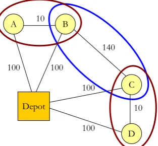
To illustrate the dynamics of the IRP, Bell et al. (1983) describe a simple example with four customers and one depot. Each customer has a fixed demand per day, a maximum capacity, and a starting inventory which is equal to its capacity; Table 2.1 displays the properties of all customers. Figure 2.1 illustrates the distances between the customers and the depot. There is one vehicle with a capacity of 5000 litres. Customers use the gas up to noon, and the vehicle starts delivering after noon. The vehicle can perform two trips per day, and we need a plan for the next two days.
Customer Daily usage (litres) Capacity (litres) Start inventory (litres) A 1000 5000 5000 B 3000 3000 3000 C 2000 2000 2000 D 1500 4000 4000
The obvious solution to this problem would be to deliver Customers A and B on the first trip and Customers C and D on a second trip, both trips on both days. We would deliver 7500 litres per day, and drive 420 kilometres per day.
A better solution is to deliver to Customers B and C on the first day, and deliver to Customers A and B, and
A B
C
D 100
100 100 100
140
10 10
Depot
to Customers C and D on the second day. Figure 2.2 illustrates this, where a circle illustrates a trip and the different colours display different days. We can deliver volume for two days to Customers A and D and for one day to Customers B and C in this solution, in a total of three trips spread out over two days. We get an average of 380 kilometres and 7500 litres per day.
Figure 2.2. Geographical display of the better solution.
Customer A B C D Total distance (km) Total volume (litres)
Trip 1 (Day 1) - 3000 2000 - 340 5000 Trip 2 & 3 (Day 2) 2000 3000 2000 3000 420 10000
Average per day 380 7500
Table 2.2. The better solution for the example.
A B
C
D 100
100 100
100
140
10 10
Depot
How VMI Can Be Successful in Gas Distribution, Peter Hulshof 13
2.2 Gas distribution
Gas is found in oil or gas fields, and it follows an intensive production process at a refinery before it is stored. From this storage, it can be supplied to depots in the market area by means of pipeline, boat, train or truck, in compressed or liquefied form. For customers that are not connected to the national grid, depots deliver gas by tank truck. This is also done for commercial customers, such as gas stations, who are selling gas to car owners. The customer stores the gas in a tank, and each customer requires a delivery between several times per week and once per year. Planners at the depots are responsible for the planning of these deliveries to make sure all customers have sufficient stock.
Figure 2.3. Forecasted weekly usage and actual weekly delivery volumes of gas in the Northern-England region in the weeks 2006-49 to 2007-48. The graph is different from
Figure 1.3, because these data only represent customers that are in the VMI program.
Figure 2.3 illustrates the annual demand curve which shows a large seasonal peak in demand in the winter months. This is caused by additional heating due to the lower temperature. The graph is constructed from actual delivery data of three depots in the Northern-England region in the UK (NE-region). These three depots serve 3.188 customers, of which 60% are in the VMI program, and deliveries are controlled by the gas company. The other 40% of the customers are not in the VMI program, and the demand of these customers is not forecasted, meaning these customers order gas themselves. We use the data of the NE-region frequently in this research.
In the graph of Figure 2.3, all customers that have no forecasted usage are excluded. This concerns (1) new customers, since there are insufficient data to determine their usage rates, and (2) customers that are not in the VMI program. Grain farms are customers that are not in the VMI program, because their demand depends on many factors that are difficult to forecast. Grain farms have a relatively large demand in the months August and September, to dry the harvested grain.
How VMI Can Be Successful in Gas Distribution, Peter Hulshof 14 Due to safety regulations, the maximum capacity at a customer is 85% of the customer’s tank capacity. An emergency delivery is scheduled, when a customer is out of stock, or nearly out of stock. The exact definition of an emergency delivery, is a delivery where the customer tank level is below 15%, and the order is added after a trip was created. There were 132 emergency deliveries in the period December 2006 until November 2007, and these are 0,8% of all orders in this period (15.929 orders). August and September have increased emergency deliveries, since grain farms have high and volatile demand in this period. Figure 2.4 illustrates the distribution of emergency orders over the year.
Figure 2.4. The number of emergency orders in the NE-region in the period December 2006 - November 2007.
Trips and restrictions
The average number of customers per trip in the NE-region is nine. This high number of stops per trip increases the complexity of calculating an optimal trip in the corresponding VRP. Many standard constraints apply to the calculation of these trips. Customers can be visited in time windows that are only bounded by the hours of daylight, and there is no need for customers to be available for the delivery. Additionally, two important restrictions apply in gas distribution: vehicle restrictions and equipment restrictions. Vehicle restrictions restrict the type of vehicle by which a customer can be visited. For instance, a customer that lives in an area that is very difficult to reach can only be visited by the smallest vehicle, since the other vehicles are too large for the roads to the customer. Equipment restrictions require certain equipment to be available in the vehicle to deliver to a customer. Although this restriction is not used in the NE-region, we add it to the solution requirements, since it is common in gas distribution.
2.2.1 The economics of gas distribution
The costs of gas distribution are mainly driven by volatility, travelled kilometres, and the number of visits to customers.
Volatility costs
Vehicle contracts are settled for a full year, so resources are fixed over the year. Volatility is a strong driver of cost, since the resources are fixed, but demand is not. Volatility is a cause for idle, or for emergency resources, and minimizing the effects of volatility is one of the objectives.
Vehicle fleet and travelled kilometres
How VMI Can Be Successful in Gas Distribution, Peter Hulshof 15 Number of visits
The number of visits to a customer should be kept to a minimum, since a visit means additional kilometres, and thus additional costs. The optimal number of visits to a customer can be calculated by dividing the customer’s usage by its capacity. This is optimal when a vehicle can only visit one customer per trip, but in gas distribution there are nine stops per trip. A customer can not be observed as an individual, but should be observed as a system, where customers in the vicinity influence the number of visits to this customer as well. This trade-off between minimizing the number of visits and minimizing the kilometres travelled is the crucial element of the IRP in gas distribution.
2.2.2 Solution requirements for gas distribution
The solution requirements for gas distribution are based on this paragraph:
(1) Travel to different areas in the region on a single day to be able to respond to emergency orders.
(2) Multi-depot approach, since a planner is usually responsible for a region with multiple depots in gas distribution.
(3) Heterogeneous fleet approach, because there are different types and sizes of vehicles in real-life instances of the IRP in gas distribution.
(4) Take in consideration vehicle and equipment restrictions. (5) Balance the workload to decrease volatility in deliveries.
2.3 ORION and SHORTREC
ORION and SHORTREC are two decision support software suites that communicate with each other by exchanging files. The suites are used by end-users at ORTEC’s clients, and they find good results with relatively low computation times.
Planners plan gas deliveries for a certain planning period, usually one day. Based on historical data of tank measurements (dip levels) and deliveries (drop sizes), ORION forecasts gas usage in the future. With the information on usage, ORION generates the orders just before a customer reaches safety stock, with the objective to minimize the number of visits. Figure 2.5 illustrates the ideal curve of a customer’s stock level.
stock level
time
maximum stock level
safety stock level
Figure 2.5. The ideal curve of a customer’s stock level to minimize the number of visits. The vertical lines are deliveries, and the diagonal lines illustrate usage. The top and bottom horizontal lines illustrate the maximum stock level and the safety stock level.
How VMI Can Be Successful in Gas Distribution, Peter Hulshof 16 Based on the orders from ORION, SHORTREC solves the VRPs for all orders that are planned on a specific day. SHORTREC produces a routing schedule that is created with a (1) constructive heuristic, and is optimized with (2) an improvement heuristic. A SHORTREC-user can select the savings-based or insertion heuristics as described in Poot et al. (2002). At the start of the algorithm, a trip is created for the customer that is farthest away from a depot. The main idea is to insert customers into this trip. These insertions come with certain costs in distance, and the customer with the lowest insertion costs is chosen. When a vehicle is filled, a new trip is started with the customer that is the farthest away from the depot. With SHORTREC, many restrictions can be taken into account: time windows, vehicle capacity, driver schedules, restricted routes, etc.
2.4 The background solution: Period Scheduler
The Period Scheduler is an algorithm that is created for the Period Vehicle Routing Problem (PVRP) for a large beverage company. This paragraph describes the Period Scheduler adjusted for gas distribution.
From the complete geographical area that is serviced by one depot, n separate seed points are chosen for every day of the planning period, so when there are five days, there are five seed points. These seed points are the centres of gravity of all customers, so they are fixed. The days of the planning period are assigned to the seed points according to their creation order, i.e. Seed 1 is assigned to Monday and Seed 2 to Tuesday, etc. See Appendix A for the detailed seed creation process.
Every customer is connected to a set of delivery scenarios, which contain percentages of the customer’s tank size that can be delivered on a certain day in the planning period. The Period Scheduler assigns one of the scenarios to the customer by solving an Integer Linear Programming problem (ILP), which is given in Appendix B. An ILP is a Linear Programming problem (LP) with a restriction to the possible values of one or more variables. The restricted variables can only be integer values. An ILP is NP-hard, where an LP is not (Garey and Johnson, 1979). An ILP where the integer restriction is ignored is called an LP relaxation. The ILP in the Period Scheduler is solved by rounding the outcome of the LP relaxation to integers.
The ILP has the objective to minimize the driving distance between the customer and the seed points, which are connected to a certain delivery day. For a ‘may-go’ customer a comparison between a delivery this week and a delivery next week is incorporated in the cost function. The cost function for not visiting the ‘may-go’ customer this week, and forwarding the delivery into the future, is given in Equation 2.1.
104 4
3
B A
ct
⋅
= for t = 6 (2.1)
How VMI Can Be Successful in Gas Distribution, Peter Hulshof 17 The workload is balanced by delivery volume per day in
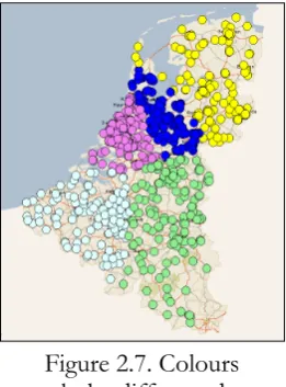
the ILP. The average expected usage per week is calculated for 13 weeks into the future, and this is set as the workload for the current week. The end-user can set the percentage of the workload that has to be delivered on every day of the week. For instance, the end-user can plan fewer orders on Friday to reserve capacity for expected pull orders. If the expected demand has an increasing curve in the next 13 weeks, we will deliver more in the current week than only the expected demand for the current week, and thus we get a moving average on the long term that takes into account the expected demand for the next 13 weeks. Figure 2.7 illustrates the customer assignment to five seed points.
2.4.1 Background solution analysis
In our solution, we consider the following aspects:
(1) The distance minimization of the Period Scheduler is a short-term perspective on cost. A long-term perspective on costs is only in the cost function for forwarding a ‘may-go’ customer by including the percentage of a ‘may-go’ customer’s capacity that can be delivered next week. Can this long-term approach also be incorporated in the cost function for delivery days within the planning period?
(2) The Period Scheduler lacks flexibility, since only one seed point is selected for each day. In case of emergencies outside the seed point’s region, it is difficult to reschedule a truck.
(3) The Period Scheduler can not cope with multiple depots in the planning region. (4) The Period Scheduler does not balance the workload considering vehicle capacity at a
depot on a certain day in the planning period, but uses manual balancing parameters. It is beneficial to connect the availability of resources to the workload that should be planned on a specific day.
2.5 Solution requirements
We describe the main requirements for our solution, based on Chapters 1 and 2:
(1) Relatively low computation times for real-life instances.
(2) The workload is balanced to cope with volatility on the short-term and the long-term. (3) Travel to different areas in the region on a single day to be able to respond to
emergency orders.
(4) Multi-depot approach, since a planner is responsible for a region with multiple depots in gas distribution.
(5) Heterogeneous fleet approach, because there are different types and sizes of vehicles in real-life instances of the IRP in gas distribution.
How VMI Can Be Successful in Gas Distribution, Peter Hulshof 18
3
Literature analysis
This chapter analyzes the literature on the IRP and seasonal peak mitigation. For the reader that is merely interested in the main insights, a summary is given in Paragraph 3.6. Paragraph 3.1 discusses key principles, which form the basis for finding a solution methodology for any type of IRP. Additionally, we discuss five solution methodologies in Paragraph 3.2. Paragraph 3.3 discusses performance measurement for the IRP, and Paragraph 3.4 illustrates the seasonal peak problem in the literature. Paragraph 3.5 discusses the available decision models that are frequently used in the literature on the IRP. The reader is referred to Appendix C for the summaries of the articles discussed in this chapter.
3.1 Key principles in solving the IRP
The key principles form a better understanding of the trade-off between long-term and short-term costs. When deliver an order earlier than its optimal delivery point?
Dror and Ball (1987)
Dror and Ball (1987) propose a short-term planning solution, in which the long-term effect of a short-term decision is reflected. They find that the relative delivery size is a key indicator of the impact of a short-term decision on the long-term cost. If the relative delivery size is small, it means the delivery size is far from optimal, and costs are higher. Their idea for relative delivery size is also used in the Period Scheduler. The relative delivery is calculated by dividing the delivery for the customer by its capacity:
Capacity
lume elivery Vo Possible D
(3.1)
Campbell, Clarke, Kleywegt, and Savelsbergh (1997)
Campbell et al. (1997) propose two assumptions to guide decisions in solving the IRP:
(1) Always try to maximize the quantity delivered, since this minimizes the number of visits to a customer on the long-term.
(2) Always try to send out a full truck load, since this maximizes utilization.
Yugang, Haozun, and Feng (2008)
Yugang et al. (2008) approach transportation cost in a way that includes distance as detour
distance, the additional distance that should be travelled if a customer is added to a trip.
This is illustrated in Figure 3.1, a trip between the Depot and Customer 1 will be: 2 * 100 = 200, and a trip including Customer 2 will be: 100 + 30 + 90 = 220. This means we increase the distance of the trip with 20.
Depot
Customer 2
Customer 1
100
30 90
How VMI Can Be Successful in Gas Distribution, Peter Hulshof 19 We state three measures for distance:
(1) Euclidean distance, distance that is given by measuring a straight line on a map between two locations.
(2) Real distance, distance that is given by measuring the minimum travel distance through a network of roads between two locations.
(3) Detour distance, distance that is given by the additional travel distance when a certain customer is inserted in an existing trip. This is measured as a real distance.
3.2 Solution methodology for the IRP
Bell et al. (1983), Federgruen and Zipkin (1984), Golden et al. (1984), and Blumenfeld et al. (1987) are among the first authors to describe a solution methodology for the IRP. Since then, researchers have defined approaches to solve the IRP for different problem instances. The main differences in these approaches are:
(1) A deterministic versus a stochastic approach, where customer usage is assumed to be either deterministic or stochastic. ORION uses deterministic customer usage.
(2) A decomposition versus an integrated approach, where a decomposition approach tries to find a solution for the IRP in a phased approach. The first phase finds a timing and quantity for a delivery, and the second phase solves the resulting VRPs. The integrated approach deals with the decision when and how much to deliver, and the VRPs, at the same time.
(3) Different decision models are used in the literature. Where most authors use an ILP to minimize cost or maximize revenue; other authors solve the IRP with Dynamic Programming (DP), or with heuristics.
All authors design solution methodologies for a homogeneous fleet. Although some methodologies cope with satellite reload facilities, no article has a multi-depot approach, where vehicles start and finish a day at multiple locations.
Golden, Assad, and Dahl (1984)
Golden, Assad, and Dahl (1984) state that the IRP is optimized along (1) a spatial dimension (distance) and (2) a temporal dimension (delivery timing). The authors use relative delivery size as a measure to reflect the temporal dimension. The distance is minimized and the relative delivery size is maximized. The authors use Equation 3.2 to select customers that have an opportunity to be delivered in a planning period.
α ≥
Capacity
lume elivery Vo Possible D
(3.2)
Dror and Trudeau (1988)
Dror and Trudeau (1988) investigate a stochastic IRP. The stochastic approach gives the opportunity to model route failures and stock outs in a simulation model. A route failure is a mismatch between the expected delivery volumes in a trip and the actual volumes, resulting in a trip with too little or too many customers. In our deterministic approach, it is difficult to test a solution for stock outs, since one can not simulate actual usage.
How VMI Can Be Successful in Gas Distribution, Peter Hulshof 20 Bard, Huang, Jaillet, and Dror (1998)
Bard et al. (1998) discuss a decomposed approach for the IRP with satellite reload facilities. The bi-criteria approach they propose is applicable to our IRP, since it combines the maximization of the relative delivery size with the objective to minimize the distance travelled. Bi-criteria problems can be approached in two ways:
(1) Both criteria are optimized simultaneously, by finding correct weights.
(2) Optimize the criteria sequentially by first optimizing one criterion and than the other.
The authors use the second, separate optimization approach, and this approach is similar to the current set-up of ORION and SHORTREC, where ORION always generates an order when safety stock is almost reached, and SHORTREC minimizes distance. Since we want to have a combination of both, we need to minimize distance, and maximize the relative delivery in one evaluation step. The authors use volume as a factor to balance the workload over the week, and every day should have an equal volume to be delivered.
Campbell and Savelsbergh (2004)
Campbell and Savelsbergh (2004) propose a methodology that is appropriate for our IRP. The methodology consists of two phases that resemble the current planning and scheduling in ORION and SHORTREC.
Phase II: Scheduling
Phase I: Planning
Cluster
generation Reducing the customer set Selection of routes
ILP 1 Set Partitioning
Critical Impending
Balance
ILP 2 Aggregation/
Relaxation
Trip construction
Insertion Heuristic
Figure 3.2. The solution methodology of Campbell and Savelsbergh (2004)
The authors reduce the problem size by creating clusters based on the knowledge that it should be possible to serve a cluster with one vehicle for a long period. They calculate the clusters once and re-calculate them when a new customer is added, or when customer usage patterns change. This form of ‘fixed pre-clustering’ requires large computation times, and is interesting in problem instances that are relatively small, since the customer set in these instances does not change often. With the high variability in customer usage curves and the many changes in the customer set in our IRP, we would update the clusters daily. We cluster in a different way, since we do want to use the distance minimization provided by clustering. ‘Must-go’ customers are the starting point for creating our clusters, since they form the basis for a solution methodology (Campbell and Savelsbergh, 2004). Clustering is also used by Jung and Mathur (2007) to minimize distances between customers before solving an actual VRP.
How VMI Can Be Successful in Gas Distribution, Peter Hulshof 21 Kleywegt, Nori, and Savelsbergh (2004)
Kleywegt et al. (2004) use an integrated approach. The authors apply Dynamic Programming (DP), where the solution space is enumerated in an intelligent way, thereby creating good results. Although their results look promising, it is not useful yet. Kleywegt et al. (2004) apply their methodology to a problem where trips consist of three stops or less, and solution times already take multiple days. Trips in gas distribution have on average nine stops, and since their computation times grow exponentially with the number of stops per trip; we can not use their solution methodology. This was noted by Campbell and Savelsbergh (2004) as well.
3.3 Performance measurement for the IRP
The IRP is an NP-hard problem, and because of its complexity, we have no optimal solution to compare our heuristic with. Usually, a lower bound can be calculated for an NP-hard problem, which is a good solution to a simple derivation of the actual problem. A lower bound for our IRP will be very weak, because the large number of customers and the large number of stops per trip result in a prohibitively large number of options to calculate (Song and Savelsbergh, 2007). Song and Savelsbergh (2007) are the only authors that study performance measurement for the IRP, and they state that volume per kilometre is the best measure to compare IRP solution methodologies for equal problem instances.
Solution performance measures
Other authors in the IRP literature define transportation cost by the factors in Table 3.1.
Factor Measure(s) Available after activity
Transported volume / Total used truck capacity
Truck utilization Scheduling
Number of trucks needed Scheduling Kilometres travelled
Distance Scheduling
Total planned volume Volume
Planning Transport cost per volume Scheduling Volume per order Planning Volume per kilometre Scheduling Working time
Driver cost Scheduling
Driving time Scheduling Relative delivery (Delivery volume / Customer Capacity)
Number of customer visits Planning
Table 3.1. Factors that influence transportation cost and measures to quantify them. Some measures are available after the planning phase, and others require the scheduling
phase to be completed as well.
3.4 Seasonal peak problem
Although some authors describe the seasonal demand peak (Dror and Ball, 1987), no author has ever written about a strategy to cope with this peak in gas distribution. Welch et al. (1971) propose five solutions for the seasonal peak in the production of gas, of which one is applicable to the distribution of gas as well.
How VMI Can Be Successful in Gas Distribution, Peter Hulshof 22 We propose two methods to mitigate the seasonal peak in demand:
(1) Take into account the future demand of all customers when assigning the orders to days. Use a workload constraint that balances the workload over a longer period than the planning period. This is also used in the Period Scheduler.
(2) Ensure customers with a large flexibility do not require a delivery in peak times, by forcing orders for these customers in quieter times. For example, customers that need one delivery per year receive a delivery in summer, to avoid deliveries when the peak is at its highest, in the middle of winter.
We study the use of Option (1) to balance the workload over a full year, because this solution methodology is connected to the IRP. The graphs in Appendix D illustrate that (2) is not used, it is recommended for future research.
3.5 Decision models to optimize the IRP solution
The IRP is frequently solved with an ILP in the literature. Next to ILP, we discuss other models that are used: Mixed Integer Linear Programming (MILP), and DP.
3.5.1 Integer Linear Programming
An ILP is NP-hard, but can be solved fast with efficient heuristics. These heuristics are found in programs like CPLEX and AIMMS, but these programs can not be implemented in our solution, since their license costs are relatively high. We must use a solver that has no license costs. To find alternative methods, we discuss branch-and-bound, Lagrangian relaxation, and rounding.
Branch-and-bound
In branch-and-bound (Winston, 1994, page 502-532) the feasible solutions to an ILP are systematically enumerated, such that the optimal integer solution is found. This is done by solving an LP relaxation, and setting the solution to the upper bound of the problem (in a maximization problem). By making use of a tree-like setup, and determining the upper bound of each node in the tree, one can determine if it is still useful to evaluate the branches that lie below a node. We can only use branch-and-bound for small problem instances, since our solver uses prohibitively long computation times for larger instances.
Lagrangian relaxation
The main idea behind Lagrangian relaxation of an ILP is to incorporate the interfering constraints into the objective function, with a certain weight or penalty if the constraint is not satisfied. The problem can be solved by finding the best weights and the lowest upper bound for the maximization problem. We do not use this method in our algorithm, since the application of Lagrangian relaxation is studied in a future graduation thesis at ORTEC.
Rounding
How VMI Can Be Successful in Gas Distribution, Peter Hulshof 23
3.5.2 Mixed Integer Linear Programming
A Mixed Integer Linear Programming problem (MILP) is an LP where a subset of the decision variables is set to binary integer variables. Usually, an MILP is solved faster than an ILP, because an MILP is less constrained. An MILP can be solved with Lagrangian relaxation and branch-and-bound.
3.5.3 Dynamic Programming
Dynamic Programming (DP) is used by Kleywegt et al. (2004). Since the computation time of their solution is prohibitively high, it is not an alternative for our solution.
3.6 Main conclusions from the literature
The literature provides us with five main insights:
(1) A decomposed approach, which separates the planning procedure from the
scheduling procedure, is better than an integrated approach. The integrated approach tries to combine planning and scheduling in one step, meaning the timing and size of the deliveries is combined with the creation of trips for all deliveries. This increases the problem’s complexity and uses a prohibitively large computation time.
(2) The long-term effect of a short-term decision can best be reflected by relative delivery size, which is the size of the delivery to a customer divided by the capacity of this customer. Relative delivery size illustrates the ‘earliness’ of an order, the lower it is, the more the delivery is pulled forward. Since pulling an order forward is costly, because it increases the number of visits to a customer, the relative delivery size should be maximized.
(3) The short-term costs are mainly driven by the distance that needs to be
travelled. This distance can be expressed in three ways: Euclidean distance, real distance, and detour distance.
(4) To have an equal workload balance on the short-term, we should balance the
total daily delivery volume in the planning period. A different balancing criterion, such as working time or travelled distance, requires an integrated approach, and a calculation of routes together with the timing of the order. Since we use a decomposed approach, we balance on volume.
(5) To mitigate the seasonal peak in demand, we balance the workload over a
How VMI Can Be Successful in Gas Distribution, Peter Hulshof 24
4
Solution
Based on Chapters 2 and 3, we design an algorithm in this chapter, which is the solution to our problem. Paragraph 4.1 summarizes the main considerations in designing the algorithm and Paragraph 4.2 illustrates the complete algorithm. Paragraph 4.3 displays the alternative designs of the algorithm. We discuss the distance types and settings of the algorithm in Paragraphs 4.4 and 4.5.
4.1 Algorithm design
We summarize the main insights drawn from Chapters 2 and 3, which show that the design has four important objectives:
(1) Create an efficient plan on the short-term, maximize the volume per kilometre. (2) Create an efficient plan on the long-term, minimize the number of visits.
(3) Balance the workload on the short-term, to use the available resources efficiently. (4) Balance the workload on the long-term, to mitigate the seasonal peak.
The volume per kilometre measures the efficiency of the plan on the short-term. The relative delivery is a measure for the long-term efficiency, the higher the relative delivery, the fewer the number of visits to this customer. The workload can be balanced on the short-term by equalizing the volume that has to be delivered per day. An equal workload balance on the long-term is achieved by calculating the average demand per period for a number of periods into the future, and delivering that volume in the current planning period. Peaks in demand are foreseen, and customers are replenished before this peak in demand.
Paragraph 4.1.1 and Paragraph 4.1.2 give the solution requirements and the assumptions that are used as input for the design of the algorithm.
4.1.1 Solution requirements
(1) Relatively low computation times for real-life instances.
(2) The workload is balanced to cope with volatility on the short-term and the long-term. (3) Travel to different areas in the region on a single day to be able to respond to
emergency orders.
(4) Multi-depot approach, since a planner is responsible for a region with multiple depots in gas distribution.
(5) Heterogeneous fleet approach, because there are different types and sizes of vehicles in real-life instances of the IRP in gas distribution.
(6) The solution is implemented and tested in the ORION and SHORTREC suites.
4.1.2 Assumptions
(1) Holding costs at the depot and at the customer are not taken into account. (2) Depots have an infinite supply of gas.
(3) Depots are not assigned to a customer; the algorithm is free to choose by which depot a customer is served.
How VMI Can Be Successful in Gas Distribution, Peter Hulshof 25
4.2 Algorithm description
We summarize the algorithm and illustrate the motivation behind the separate steps in Paragraph 4.2.1 and Figure 4.1. Paragraph 4.2.2 describes the algorithm in detail.
4.2.1 Algorithm overview
We start the algorithm with a set of customers, with certain start inventories and historical data, to calculate future usage. We finish the algorithm with a set of planned orders for a selection of these customers, on specific days in the planning period.
Step 1: Customer selection
We select the set of customers for the algorithm. We only select those customers that can at least receive a relative delivery size of α.
Motivation: To minimize the long-term cost, we have to minimize the number of visits to each customer. A high relative delivery size decreases the number of visits, since the optimal relative delivery size is 100% (Dror and Ball, 1987; Golden et al., 1984).
Step 2: Flexible clustering
We create clusters based on the set of ‘must-go’ customers.
Motivation: To minimize short-term cost, we have to minimize the distance travelled. By creating clusters based on distance, we aim to minimize the travelled distance (Campbell and Savelsbergh, 2004; Jung and Mathur, 2007).
Step 3: Generate schedules
We generate all possible delivery schedules for the customers that are in a cluster. A delivery schedule contains the relative delivery sizes per day of the planning period. For ‘may-go’ customers, it also contains a relative delivery size that corresponds with the end of the following planning period.
Motivation: The ILPs in Steps 4 and 5 need these schedules as input.
Step 4: Assignment of seed customers with an ILP
An ILP assigns seed customers to delivery schedules. The ILP plans all seed customer deliveries on a specific day and balances the number of seed customer deliveries over the depots and the planning period, with regards to the available vehicle capacity.
Motivation: The ILP has the objective to minimize the long-term cost by maximizing the relative delivery size (Dror and Ball, 1987; Bard et al., 1998). The number of seed deliveries is balanced, and not the volume, since we want to spread out the number of clusters, and thus the number of seeds, over the planning period. The volume is balanced in Step 5.
Step 5: Assignment of clustered customers with an ILP
An ILP assigns clustered customers to delivery schedules. The ILP plans all customer deliveries on a specific day in this step and balances the total volume of seed customer deliveries and clustered customer deliveries over the planning period, with regards to the available vehicle capacity.
How VMI Can Be Successful in Gas Distribution, Peter Hulshof 26
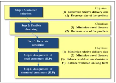
Step 1: Customer selection
Step 2: Flexible clustering
Step 3: Generate schedules
Step 4: Assignment of seed customers (ILP)
Step 5: Assignment of clustered customers (ILP)
Objectives: (1) Maximize relative delivery size (2) Decrease size of the problem
Objectives: (1) Minimize travel distance (2) Decrease size of the problem
Objectives: (1) Maximize relative delivery size (2) Minimize travel distance (3) Balance workload on short-term (4) Balance workload on long-term
Figure 4.1. An overview of the steps in the algorithm and their objectives.
4.2.2 The algorithm in detail
This paragraph explains the details of the separate steps in the algorithm and presents mathematical models that are used. Appendix E illustrates all mathematical symbols that are used in this chapter.
4.2.2.1 Step 1: Customer selection
The driver for long-term costs in the IRP is relative delivery size (Golden et al., 1984; Dror and Ball, 1987). The relative delivery size is given in the left term of Equation 4.1, and to maximize it, we choose to only consider customers that can receive a relative delivery above α. This is the approach of Golden et al. (1984).
α ≥
Capacity
lume elivery Vo Possible D
(4.1)
In Equation 4.1, maximum stock is the capacity of the customer’s tank that can be used because of safety reasons and regulations, and it is 85% of the total capacity of the customer’s tank. We can not set α too high, since it would result in stock outs.
‘Must-go’ customers
How VMI Can Be Successful in Gas Distribution, Peter Hulshof 27 4.2.2.2 Step 2: Flexible clustering
In order to minimize travel distance, clustering is a tool that is widely applied in the literature (Campbell and Savelsbergh, 2004; Jung and Mathur, 2007). Clustering is done based on distance between a customer and a certain reference point, which is called a seed.
In the literature, clustering is usually done before the actual planning phase and is no daily activity of a planner. In a large customer set, information on the customer base changes continuously, thus to ensure that clusters are up to date, clustering should be part of the planning process. In our solution, clusters are created in a fast procedure, by selecting a seed and adding other customers to this seed’s cluster. The closest customer is added first, and we add customers until the distance between a customer and the seed is above a certain threshold. All customers that are in the selection of customers can be selected into the clusters, including ‘must-go’ customers. These flexible clusters are computationally fast and based on the latest knowledge about the customer base.
The ‘must-go’ customers form the foundation of the problem (Campbell and Savelsbergh, 2004) and are therefore the basis for creating the clusters. The ‘must-go’ customer list is sorted, and the first customer on the sorted ‘must-go’ customer list is selected as a seed for the first cluster. We proceed until we have clustered all ‘must-go’ customers, either as a seed for a cluster or a customer that is selected in a cluster. A cluster can not include customers that were clustered earlier.
Sorting the ‘must-go’ customer list
The ‘must-go’ customer list is sorted on three criteria, which are explained in detail later:
(1) The number of days between the start of the planning period and the latest day of delivery of the customer: in ascending order.
(2) The number of deliveries for a customer in the planning period: in descending order. (3) The number of vehicle types that can visit the customer: in ascending order.
Rank Customer Days between start of planning period and delivery
Number of deliveries in planning period
Number of vehicle
types
1 Customer A 3 2 1
2 Customer B 3 2 >1
3 Customer C 3 1 >1
4 Customer D 4 1 1
5 Customer E 4 1 >1
Table 4.1. An example of a sorted ‘must-go’ customer list.
Table 4.1 illustrates a sorted ‘must-go’ customer list with five ‘must-go’ customers. Customers on the ‘must-go’ customer list can also be selected in a cluster. To optimize the use of clusters, we do not want a customer in a cluster to have a latest delivery date
earlier than the seed of that cluster, because that would cause problems in assigning the
How VMI Can Be Successful in Gas Distribution, Peter Hulshof 28 A customer that requires multiple deliveries in the planning horizon should be a seed customer, since the size of its cluster is larger to be able to deal with the multiple deliveries. This is explained in the part on cluster constraints below.
Additionally, we want to select the most restricted customers as a seed first, because it makes it easier to combine several ‘must-go’ customers into one cluster. All customers can be added to a seed that can be visited by only one vehicle type, and fewer customers can be added to a seed that can be visited by all vehicles. This is explained in the part on restrictions below.
Restrictions
In Paragraph 2.2, we pointed out that vehicle and equipment restrictions are specific to gas distribution. For both of these restrictions there is a simple rule to follow in creating the flexible clusters. The seed of a cluster is the most important customer in the cluster, since it is the ‘must-go’ customer on which the cluster is founded. To make sure that a complete cluster can be visited by one vehicle, we need to make sure the vehicle that will visit the seed customer can also visit all the other customers in the cluster. This simple rule makes it easy to evaluate if a certain customer can be added to a cluster.
Cluster constraints
Constraint parameters for the clusters are used. A maximum distance between the seed and the customer will ensure proximity of clustered customers to the seed customer. A minimum and maximum number of customers in one cluster are used to control the size of the cluster. This minimum and maximum number of customers is multiplied by the number of required deliveries of the seed customer to ensure the cluster is large enough.
Number of seeds per day
Additionally, we ensure that every day has at least one or more seeds, by first generating one or more clusters for every day in the planning period. We select the first ‘must-go’ customer on the list which has a latest delivery day that matches the day in the planning period, for which we are currently selecting a seed customer. We proceed with the next day in the planning period with the same procedure. If there are no ‘must-go’ customers left for a certain day, a ‘may-go’ customer may be selected as a seed customer. It is beneficial to find multiple seeds per day in the planning period, since this geographically spreads the customers throughout the region, which is good to handle emergency deliveries, and which helps in balancing the workload throughout the region for the depots.
4.2.2.3 Step 3: Generation of schedules
After clustering, there are seed customers and clustered customers. We have selected these customers on relative delivery size and on distance to the seed customers. All customers that are not selected or not clustered are not considered further to keep the problem small and tractable.
How VMI Can Be Successful in Gas Distribution, Peter Hulshof 29 The schedules F333 are for a ‘may-go’ customer with no delivery window on Sunday, and the 86% in the schedule with index 7 indicates that if the customer is not visited in this planning period, the customer requires a delivery of 86% of its maximum capacity by the end of the next planning period.
Schedule Index Monday Tuesday Wednesday Thursday Friday Saturday Sunday End of next planning period
F111 1 75% 35% 0 0 0 0 0 0
F111 2 75% 0 50% 0 0 0 0 0
F111 3 75% 0 0 65% 0 0 0 0
F222 1 60% 0 0 0 0 0 0 0
F222 2 0 65% 0 0 0 0 0 0
F222 3 0 0 0 75% 0 0 0 0
F333 1 50% 0 0 0 0 0 0 0
F333 2 0 53% 0 0 0 0 0 0
F333 3 0 0 56% 0 0 0 0 0
F333 4 0 0 0 59% 0 0 0 0
F333 5 0 0 0 0 62% 0 0 0
F333 6 0 0 0 0 0 65% 0 0
F333 7 0 0 0 0 0 0 0 86%
Table 4.2. An example with 13 schedules illustrating the delivery percentages per day in the planning period.
4.2.2.4 Step 4: Schedule assignment with an ILP for seed customers
Seed customers are the distance reference points for assigning the clustered customers in Step 5, thus we assign the seed customers to schedules first.
An ILP is used to assign the seed customers to a schedule. The schedules are connected to a certain day of delivery, or when there are multiple deliveries for a customer in the planning period, to certain days of the planning period. A seed customer is nearly always a ‘must-go’ customer, and a seed customer can not be forwarded to a following period, since we need the seed customers as a distance reference for the clustered customers.
We want to balance the number of clusters per day and per depot throughout the planning period, to ensure efficient use of capacity. Therefore we balance the number of seed deliveries, and not their delivery volume. We use seed deliveries, and not seed customers, since a seed customer may have multiple deliveries in the planning period.
Workload calculation
Appendix F explains these procedures in detail, but we explain the concepts here. We balance the number of seed deliveries over the planning period and over the depots, and the maximum workload is calculated by multiplying the total number of seed deliveries with the fraction of the total available vehicle capacity in the planning period, that is available at the specific depot, on the specific day. We select the maximum of this workload, and the expected number of seed deliveries for a depot and a day to ensure the problem is feasible. We can add a certain percentage of the maximum workload that can be used as a bandwidth for feasibility, but we do not use it in this part of the thesis.