Design of molecules and materials for applications in clean
energy, catalysis and molecular machines through quantum
mechanics, molecular dynamics and Monte Carlo simulations
Thesis by
Jose L. Mendoza-Cortes
In Partial Fulfillment of the Requirements for the Degree of
Doctor of Philosophy
California Institute of Technology Pasadena, California
2012
c
2012
Acknowledgments
I am in debt to my advisor Prof. William A. Goddard for his patience and discussions during my doctoral studies. I am deeply thankful to him for allowing me to pursue an independent way of doing research and showing me how to be a better scientist.
I would like to thank also many collaborators during these years: Prof. Omar M. Yaghi, Dr. Hiroyasu Furukawa, Dr. Ravinder Abrol, Dr. Andres Jaramillo-Botero, Dr. Robert Nielsen, Dr. Tod A. Pascal and Prof. Theodor Agapie. I learnt many things about science through discussions with them.
My special thanks to Prof. Yaghi, who has been an exemplary scientist and helped me to improve as a scientist. I also would like to thank Dr. Furukawa who was patient and tough enough with his vast experience.
I would like to acknowledge some of my colleagues for fruitful discussions about different scientific topics; Dr. Jamil Tahir-Kheli, Wei-Guang Liu, Ted Yu, Fan Liu, Ross Fu, Jacob Kanady, Emily Y. Tsui, Vaclav Cvicek and Hai Xiao. It is amazing how much you can learn by discussing with your colleagues.
Also I would like to thank the support of my friends over the years; there are many of them spread over the world but specially Jorge Cholula, currently in Germany and Naoki Aratani from Japan. I would like to thank Ernie Mercado for allowing me to have some Mexican food on campus. My gratitude to the California Institute of Technology which provided me with fellowship during my first year and also to the Roberto Rocca Program for providing support for two years.
Abstract
Contents
Acknowledgments iv
Abstract v
List of Tables xiii
List of Figures xxi
1 Introduction 1
2 Prediction of Structures of Metal-Organic Complex Arrays (MOCA) 7
2.1 Introduction . . . 7
2.2 Method I: QM/MM . . . 8
2.2.1 Methodology . . . 8
2.2.2 Quantum Mechanical Calculations . . . 8
2.2.2.1 The case of Platinum (Pt) . . . 9
2.2.2.2 The case of Rhodium (Rh) . . . 11
2.2.2.3 The case of Ruthenium (Ru) . . . 12
2.2.2.4 Dimers . . . 14
2.2.3 Structures Obtained from QM/MM . . . 17
2.2.4 Conclusions . . . 19
2.3 Method II: Structure Prediction Inspired in Enzymes . . . 20
2.3.1 Methodology . . . 20
2.3.2 Generation of Conformers for All Compounds . . . 20
2.3.3 Conclusions . . . 24
3 Coarse-Grained Potential for Hydrogels from Quantum Mechanics 26 3.1 Introduction . . . 26
3.2 Methodology . . . 27
3.2.2 The Finite Extensible No Linear Elastic (FENE) Potential . . . 27
3.3 FENE Potential . . . 28
3.3.1 Dihedral Conformation and the FENE Potential . . . 29
3.3.1.1 Quantum Mechanics for the Dihedral Angles in the [aam-aam] Dimer 29 3.3.1.2 Quantum Mechanics for the Dihedral Angles in the [xlinker] Monomer 31 3.3.2 Bond Strength and the FENE Potential . . . 32
3.3.2.1 Quantum Mechanics of [aam-aam] . . . 32
3.3.2.2 Quantum Mechanics of [amps-aam] . . . 33
3.3.2.3 Quantum Mechanics of [amps-amps] . . . 34
3.3.2.4 Quantum Mechanics of [xlinker] . . . 36
3.3.2.5 Quantum Mechanics of [xlinker-xlinker] . . . 37
3.3.2.6 Quantum Mechanics of [xlinker-aam] . . . 38
3.3.2.7 Quantum Mechanics of [xlinker-amps] . . . 39
3.3.3 Conclusions . . . 40
3.4 Reaction Rates from Transition State Theory . . . 43
3.4.1 Reaction Rates in Gas Phase and Water . . . 44
3.4.2 Conclusions . . . 46
4 Origin of the Positive Cooperativity in the Template-Directed Formation of Molecular Machines 48 4.1 Introduction . . . 48
4.2 Methodology . . . 49
4.3 Results and Discussion . . . 50
4.3.1 Experimental Coordinates vs MM vs QM . . . 50
4.3.2 Origin of the Positive Cooperativity . . . 51
4.3.3 Role of the Counter Anion . . . 55
4.4 Conclusions . . . 60
5 Design of New Models for the Oxygen Evolving Complex 62 5.1 Introduction . . . 62
5.2 Methodology . . . 64
5.3 Results and Discussion . . . 64
5.3.1 Validation of the Computational Methodology: Geometry . . . 64
5.3.2 Validation of the Computational Methodology: Redox Potentials . . . 67
5.3.3 Prediction of New Models that Resemble the OEC Both Structurally and Electronically . . . 70
6 Methane Storage in Metal-Organic Frameworks and Covalent-Organic
Frame-works 73
6.1 Adsorption Mechanism and Uptake of Methane (CH4) in Covalent-Organic
Frame-works: Theory and Experiment . . . 73
6.1.1 Introduction . . . 73
6.1.2 Methodology . . . 76
6.1.2.1 Force Field . . . 76
6.1.2.2 QM Determination of the vdW Force Field Parameters . . . 77
6.1.2.3 GCMC Procedure . . . 80
6.1.2.4 Structural Characteristics of COFs . . . 80
6.1.3 Results and Discussion . . . 80
6.1.3.1 Comparison Between Theoretical and Experimental Methane Ad-sorption . . . 80
6.1.3.2 Gravimetric Methane Uptake in Other COFs . . . 82
6.1.3.3 Adsorption Mechanism of Methane in COFs . . . 84
6.1.3.4 Isosteric Heat of Adsorption . . . 84
6.1.3.5 Delivery Amount in COFs . . . 87
6.1.4 Concluding Remarks . . . 87
6.2 Design of Covalent Organic Frameworks for Methane Storage . . . 89
6.2.1 Introduction . . . 89
6.2.2 Methodology . . . 90
6.2.2.1 Force Field . . . 90
6.2.2.2 Electrostatic Interactions . . . 91
6.2.2.3 Grand Canonical Monte Carlo . . . 91
6.2.2.4 Molecular Dynamics . . . 92
6.2.2.5 Topological Consideration in the Design of COFs . . . 92
6.2.3 Results and Discussion . . . 92
6.2.3.1 Delivery Volumetric Uptake in Designed COFs . . . 92
6.2.3.2 Isosteric Heat of Adsorption . . . 94
6.2.3.3 Stability of COFs . . . 95
6.2.3.4 Comparisons to Previous Computational Studies . . . 97
6.2.4 Concluding Remarks . . . 98
7 Clean Energy (H2) Storage in Metal-Organic Frameworks and Covalent-Organic
7.1 High H2Uptake in Li-, Na-, K- Metalated Covalent-Organic Frameworks and
Metal-Organic Frameworks at 298 K . . . 100
7.1.1 Introduction . . . 100
7.1.2 Computational Details . . . 101
7.1.2.1 Quantum Mechanics Calculations and Development of the Parame-ters for Nonbond Interactions . . . 101
7.1.2.2 Valence Bond Force Field . . . 102
7.1.2.3 Grand Canonical Monte Carlo Loading Curves . . . 102
7.1.3 Results and Discussion . . . 103
7.1.3.1 Nature of the Chemical Bond for the Li-Benzene (Li-Bz) Systems . 103 7.1.3.2 Gravimetric Uptake . . . 106
7.1.3.3 Volumetric Uptake . . . 110
7.1.3.4 Isosteric Heat of Adsorption . . . 113
7.1.3.5 Adsorption Mechanism of Molecular Hydrogen . . . 113
7.1.3.6 Comparisons to Previous Computational Studies . . . 115
7.1.4 Concluding Remarks . . . 116
7.2 Dependence of the H2Binding Energies Strength on the Transition Metal and Organic Linker . . . 117
7.2.1 Introduction . . . 117
7.2.1.1 Types of Interactions for H2 . . . 117
7.2.1.2 Langmuir Theory and the Optimal Enthalpy . . . 119
7.2.2 Computational Details . . . 121
7.2.3 Results and Discussion . . . 122
7.2.3.1 Current Linkers Used in Porous Frameworks . . . 122
7.2.3.2 Proposed Linkers Based on Experimental Crystal Structures . . . . 132
7.2.3.3 Alternative Strategy to Metalate COFs and MOFs . . . 135
7.2.4 Concluding Remarks . . . 138
Appendix 139 A Quantum Mechanical Calculations and Geometries on the Formation of Molecu-lar Machines 140 A.1 All QM Calculations . . . 140
A.2 Geometries for the R Family (2R-D-2PF6, 1R-D-2PF6, 2R-D-2PF6) and for the R’ Family (2R-Dp-2PF6, 1R-Dp-2PF6, 2R-Dp-2PF6) . . . 144
A.2.1 2R-D-2PF6-M06L . . . 144
A.2.3 0R-D-2PF6-M06L . . . 154
A.2.4 2R-Dp-2PF6-M06L . . . 157
A.2.5 1R-Dp-2PF6-M06L . . . 163
A.2.6 0R-Dp-2PF6-M06L . . . 168
B Generalization of the Sorption Process with Multilayers for Non-Self-Interacting Atoms and Molecules 171 B.1 Given a Topology . . . 171
B.2 Determine the Occupancy . . . 171
B.3 Gibbs Ensemble . . . 172
B.3.1 Monolayer Theory . . . 173
B.3.2 Restricted Multilayer Theory . . . 175
B.4 Hydrogen Molecule Case . . . 176
B.4.1 Monolayer Theory in H2 . . . 176
B.4.2 Multilayer Theory in H2 . . . 176
B.5 Supplementary Information . . . 179
B.5.1 NIST Data for H2 . . . 179
List of Tables
1.1 Ensembles for statistical mechanics. Estands for energy of the state; T, temperature;
V, volume;N, number of particles;µ, chemical potential. β is given by 1/(kT), where
k is the Boltzmann constant. The denominators Ω, Q, Ξ and ∆ are the partition
functions for each ensemble. . . 4
2.1 DFT energies for the Rhcis andtrans . . . 11
2.2 Binding energies (Ebind) for the different dimers obtained from DFT/MO6-2X and basis set LACVP**/6-31G** . . . 14
2.3 Energies for the top 10 conformers. R stands for rank. All the energies are in kcal/mol. 22 3.1 Energies for dihedral in the aam-aam . . . 30
3.2 FENE parameters obtained for different dihedral for the [aam-aam] dimer . . . 31
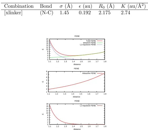
3.3 [xlinker] FENE parameters for the FENE potential from QM . . . 32
3.4 [aam-amps] FENE parameters for the FENE potential from QM . . . 34
3.5 [amps-amps] parameters for the FENE potential from QM . . . 35
3.6 FENE parameters . . . 37
3.7 [xlinker-xlinker] parameters for the FENE potential from QM . . . 37
3.8 [xlinker-aam] parameters for the FENE potential from QM . . . 39
3.9 [xlinker-amps] parameters for the FENE potential from QM . . . 40
3.10 All the parameters for the FENE potential from QM. I and II stand for different explored C-C bonds . . . 42
3.11 Parameters for water . . . 45
3.12 Free energy (G) of all the reactions in gas phase. Energies are in kcal/mol. . . 47
3.13 Free energy obtained from QM and the derived reaction constant (k) from TST . . . 47
4.3 Root mean square distance (RMSD) for the comparison between experimental structure for 2R·2PF6 and the QM and MM methods. Column 2 and 3 shows the estimation of the R(π−π) interaction for benzene (Bz) in the stopper of the dumbbell (D), first rotaxane (R1) and second rotaxane (R2) . . . 52 4.4 Comparison of binding energies for the Formation of 1R-2PF6 and 2R-2PF6. All the
units are in kcal/mol. . . 52 4.5 ∆Ggasand ∆Gsolv with respect to isolated rotaxanes rings and dumbbell. The solvent
used is CH3CN. All the units are in kcal/mol. . . 55 4.6 ∆Ggasand ∆Gsolvwith respect to isolated rotaxanes rings and dumbbell. All the units
are in kcal/mol. . . 58 4.7 Dipole moments (µ, /Debye) obtained from Electrostatic potential (ESP) charges and
Mulliken charges. The ESP and Mulliken charges have been normalized. . . 59
5.1 Oxidation/reduction potentials for the Mn3CaO4compound with respect to ferrocene/ ferrocenium. Solvents: dimethylacetamide (DMA) and dimethylformamide (DMF). . . 68 5.2 Oxidation/reduction potentials for the Mn4O4 compounds with respect to ferrocene/
ferrocenium. Solvent: dimethylacetamide (DMA). . . 69 5.3 Bond distances for the fourth Mn shown and its first coordination shell as it is shown
in Figure 5.7. . . 70
6.1 Pore size (PSize), surface area (SA), pore volume (VP), and density of the Framework without guest molecules (ρ) for the studied COF series . . . 76 6.2 Nonbonded FF parameters developed to fit the RI-MP2 calculations . . . 78 6.3 Most-stable interaction geometries for clusters considered in this work . . . 79 6.4 Isosteric heat of adsorption (Qst), surface area (SA), pore volume (VP), and uptake of
the framework series at 298 K (Where Tot = total, Exc = excess, and Del = delivery) 95 6.5 MD statistics for the frameworks obtained at 298 K . . . 97
7.1 Properties of the frameworks used in this work: surface area (SA), pore volume (VP), and density (ρ) . . . 101 7.2 Nonbonded FF parameters used for this study based on MP2 for Li and CCSD(T) for
Na and K . . . 102 7.3 Electronic energy for the optimized systems using different basis sets (6-31G**++ and
6-311G**++) and different functionals (M06 and B3LYP) is presented . . . 104 7.4 Zero-point energy (ZPE), vibrational enthalpy (Hvib), total enthalpy (Htot), vibrational
7.5 Different interactions H2 can have with other entities that can be used to tune the ∆H◦
ads . . . 118 7.6 DOE targets for H2 storage system for light-duty vehicle and the estimation of the
optimal ∆H◦
ads under these conditions using the Langmuir model . . . 120 7.7 Delivery amount obtained using ideals ∆H◦
ads and different temperatures . . . 121 7.8 Binding energies (∆H◦bind) obtained for the ground state of linkerBBHand different
number of physisorbed H2. We also show ∆H◦bind for the linker + TM(n)Cln + H2. The H-H bond of isolated H2is 0.741 ˚A . . . 123 7.9 Binding energies (∆H◦bind) obtained for the ground state of linkersPIPandPIPEand
different number of physisorbed H2. We also show ∆H◦bindfor the linker + TM(n)Cln + H2. The H-H bond of isolated H2 is 0.741 ˚A . . . 127 7.10 Binding energies (∆H◦bind) obtained for the ground state of linker PIAand different
number of physisorbed H2. We also show ∆H◦
bind for the linker + TM(n)Cln + H2. The H-H bond of isolated H2is 0.741 ˚A . . . 130 7.11 Binding energies (∆H◦bind) obtained for the ground state of linkerBPYand different
number of physisorbed H2. We also show ∆H◦
bind for the linker + TM(II)Cl2 + H2. The H-H bond of isolated H2is 0.741 ˚A . . . 132 7.12 Binding energies (∆H◦bind) obtained for the ground state of linkerBPYMand
differ-ent number of physisorbed H2. We also show ∆H◦bind for the linker + TM(II)Cl2 + H2. The H-H bond of isolated H2is 0.741 ˚A . . . 134 7.13 Binding energies (∆H◦bind) obtained for the ground state of all linkers (BBH, PIP,
PIPE, PIA,BPY, andBPYM) + Pd shown in Figure 7.19 reacting with different number of H2. For each case the spin is 0. The H-H bond of isolated H2is 0.741 ˚A . . 137
A.1 Free energies in gas and solvated phase including quantum corrections. The solvent used is CH3CN. Units:kcal/mol . . . 141 A.2 Electronic Energy (E,scf), Zero Point Energy (ZPE), Solvation energy for CH3CN
(Esolv). Units:kcal/mol . . . 142 A.3 Free energies in gas and solvated phase including quantum corrections. The solvent
used is CH3CN. Units:kcal/mol . . . 143 A.4 Electronic Energy (E , scf), Zero Point Energy (ZPE), Solvation energy for CH3CN
List of Figures
1.1 Theoretical multiparadigms. (a) was adapted from [1], (b) is courtesy of Julius Su, and
Part (c) is courtesy of Andres Jaramillo-Botero. . . 3
1.2 Uptake for CH4 for COFs and MOFs and observation of the sorption mechanism for the uptake . . . 5
1.3 The design of two new COFs that overcome the DOE target at room temperature. They perform better than MOF-177, currently on the market. . . 6
1.4 MOF200-Li and COF102-Li reach the 2015 DOE target. . . 6
2.1 Metal-organic complex arrays (MOCA). QM was used for the black part, including the metal. MM was used for the pink part. Fmoc stands for fluorenylmethyloxycarbonyl. 9 2.2 Structures used for the QM calculations. For the calculations in gas phase we did not use the counter anion but the absolute charge that is shown. . . 10
2.3 Coordinate scan for the dihedrals CCCC and CCCO of the Pt case. The pink lines indicate the dihedral angle used. . . 11
2.4 Different dihedral angles tested for the Rh complex. The pink lines indicate the dihedral angle used. . . 12
2.5 Ru complex . . . 13
2.6 3D-representation of the optimized structure obtained for each of the dimers considered in this study. . . 17
2.7 Final configuration obtained using the QM/MM method for all the arrays denominated MOCA A, B, C, D, E and F . . . 20
2.8 Population of all conformers generated for MOCA A to F . . . 21
2.9 Population of conformers generated for Compound A, B, C, D, E and F . . . 22
2.10 Top 1st conformer for all compounds obtained by using method II . . . 25
3.2 All monomers used are presented: (a) acrylamide (71.08) (b) 2-acrylamido-2-methyl propane sulfonate−1 (206.24 g/mol) (c) sodium 2-acrylamido-2-methyl propane
sul-fonate (229.23 g/mol) and (d) N,N’-methylenediacryl amide(154.17 g/mol). . . 29
3.3 The dihedral used for the aam-aam dimer is shown in (a) and (b) with magenta and green colors, respectively. The 360◦ point should be equivalent to the O◦ for a con-strained dihedral scan, however we executed a relaxed scan. . . 29
3.4 Bond energies for aam-aam with dihedrals 173.9◦ and 179.4◦ . . . 30
3.5 xlinker dihedral used. (a) The structure used is shown in red and the dihedral angle explored is magenta. (b) 3D representation of the xlinker with the dihedral used shown in green. The blue dots in (c) are reoptimized structures with the dihedrals shown in green. . . 31
3.6 Bond scan for most stable xlinker dihedrals . . . 32
3.7 Bond strength for a used conformation of aam-aam . . . 33
3.8 [aam-aam] FENE potential for structures in Figure 3.7 . . . 33
3.9 amps-aam used. The scan used is shown with a magenta arrow. . . 34
3.10 [amps-aam] FENE potential for structures in Figure 3.9 . . . 34
3.11 amps-amps neutral and anion used. The scan used is shown with a magenta arrow. . 35
3.12 [amps-amps] FENE potential for structures in Figure 3.11 . . . 36
3.13 xlinker used. The scan used is shown with a magenta arrow. . . 36
3.14 [amps-amps] FENE potential for structures in Figure 3.13 . . . 37
3.15 xlinker-xlinker used. The C-C bond scan used is shown with a magenta arrow. . . 38
3.16 [amps-amps] FENE potential for structures in Figure 3.15 . . . 38
3.17 xlinker-aam used. The scan used is shown with a magenta arrow. . . 39
3.18 [xlinker-aam] FENE potential for structures in Figure 3.17 . . . 40
3.19 xlinker-amps used. The scan used is shown with a magenta arrow. (b) and (e) are equivalent. . . 41
3.20 [xlinker-aam] FENE potential for structures in Figure 3.19 . . . 41
3.21 All QM results around the equilibration point . . . 42
3.22 For all studied reactions, the free radical polymerization mechanism is assumed . . . . 45
3.23 This plot shows the product (left) and reactant (right) . . . 45
4.1 Reaction for the template directed formation of rotaxanes for the (a)RFamily and for the (b)R’family . . . 49
4.3 Compounds for the R family (a,b and c; xR-D-2PF6) and for the R’ family (d,e and f; xR-Dp-2PF6). Colors are C: grey, O:red, N:blue, F: green, P:purple and H:not shown. rotaxanes are colored in full red in order to distinguish them from the atoms in the dumbbell. . . 52 4.4 Distances for the optimized structure for the (a) 2R-D-2PF6 (R family) and for (b)
2R-Dp-2PF6 (R’family). In the R family we observe rotaxane-rotaxane interaction while in the R’ family, the distance between rotaxane rings is too large for them to interact. Distance between stopper and rotoxane ring is marked in black. Distance between first and second rotoxane is marked in red. Distance between first and second -NH2- site is marked in blue. The optimal rotaxane-rotaxane interaction distance is 3.6 ˚A. . . 55 4.5 xR-D-2anion compounds. . . 56 4.6 xR-Dp-2anion compounds. . . 57 4.7 Free energies in the gas phase for (a) gas phase and (b) solvated phase for the R
Family: 2R-D-2PF6 and 2R-D-2F (top) and for theR’Family: 2R-Dp-2PF6 and 2R-Dp-2F (bottom). The positive cooperativity is only observed with the PF−6 (or I−, not shown) counter anion. . . 58 4.8 Dipole moments (µ) from ESP charges obtained for the (a)RFamily (2R-D-2PF6and
2R-D-2F) and for the (b)R’family (2R-Dp-2PF6 and 2R-Dp-2F) . . . 60
5.1 (a) Fundamental chemical reactions that take place in the production of O2 that start with the conversion of solar energy (hν) to an electron and a hole in the chlorophyll center called P680. (b) The catalytic cycle of the Oxygen-evolving complex (OEC) is shown where every oxidation is defined as a S-state (Sn). (Inset) The full description of the OEC is shown. . . 63 5.2 Complexes synthesized in the Agapie group containing (left) a Mn3Ca and (right) a
Mn4 cubane. Notice how the Ca in Mn3 at the top have been substituted by one Mn to give Mn4. . . 63 5.3 Comparison of geometries obtained from experiment (colored: Ca; magenta, Mn; light
5.4 Comparison of geometries obtained from experiment (colored: Ca; magenta, Mn; light blue, O; red, C; grey, H; white) and theory (black) using the simplified ligand. We show the root mean square (RMS) to compare all the atoms in the structure (top) and the cubane (bottom). The structures with this simplified ligand are almost identical to the ones obtained with the full ligand (Figure 5.3). . . 66 5.5 Oxidation/reduction for the Mn3CaO4compound. Color code: Ca; magenta, Mn; light
blue, O; red, C and H; black. . . 68 5.6 Oxidations/reductions for the Mn4O4 compound. Color code: Ca; magenta, Mn; light
blue, O; red, N; dark blue, C and H; black . . . 69 5.7 New models for the OEC that includes the fourth Mn giving a CaMn4O4type cluster;
(a) CaMn4-NH2, similar to S1 (b) CaMn4-bipy, similar to S1 and (c) CaMn4-acac, similar to S2. Color code: Ca; magenta, Mn; light blue, O; red, N; dark blue, C; black and H; grey . . . 71
6.1 Molecular structures of building units used for COF synthesis (outside black box) and their COF formation reactions (green box, boroxine; blue box, ester) . . . 75 6.2 Atomic connectivity and structure of crystalline products for (a) 2D-COFs and (b)
3D-COFs. Unit cells are shown in blue lines. Atom colors: C, black; O, red; B, pink; Si, yellow; H, blue . . . 77 6.3 Comparison of the optimized FF energies with QM (MP2-RI) for four configurations:
(a) CH4-CH4; (b) C6H6-CH4; (c) B3O3H3-CH4; (d) Si(CH4)4-CH4. FF results are shown as dashed lines while the QM results are shown by empty symbols. Each con-figuration has four plausible geometrical structures shown to the right, where C atoms are brown, B pink, O red, Si yellow, and H white. Configurations interacting through the edges are not shown. The insets show the accuracy in fitting to the equilibrium distance. Data plotted here as the BSSE corrections are included in the Supporting Information. . . 79 6.4 Predicted (open triangles) and experimental (closed circles) methane isotherms at 298 K
in excess uptake gravimetric units (wt %): (a) COF-5; (b) COF-8. The total predicted uptake is shown by open squares. . . 81 6.5 Predicted gravimetric methane isotherms at 298 K: (a) total and (b) excess uptake
6.6 Ensemble average from the GCMC steps for methane adsorption in 2D-COFs at various pressures. Atom colors are the same as in Figure 6.2; the average of the methane gas molecules is shown in blue. The accessible surface is shown in purple and was calculated using the vdw radii of every atom of the framework and the methane kinetic radii: (a) COF-10, pore diameter = 35 ˚A; (b) COF-5, pore diameter = 27 ˚A; (c) COF-8, pore diameter = 16 ˚A; (d) COF-6, pore diameter = 11 ˚A. . . 85 6.7 Ensemble average of methane molecules at different pressures: (a) 103; (b)
COF-105; (b) COF-108. Atom colors: C, gray; O, red; Si, yellow; B, pink. The average of the methane gas molecules is in blue. The accessible surface was calculated as in Figure 6.6. COF-102 has the same sorption profile as COF-103 and it is not shown. . 86 6.8 (a)PredictedQst values for COFs as a function of pressure. We have added the
calcu-lated values for MOF-177 for comparison. (b) VP versusQst for COFs. There are two groups, based on the structural analysis: 2D-COFs (-1, -5, -6, -8, -10), which laid in a line with the same slope. Also the 3D-COFs (-102, -103, -105, -108) have a common line. Both lines coincide at VP ∼1.53 cm3/g andQ
st ∼10.6 kJ/mol. . . 86 6.9 Predicted volumetric methane isotherms at 298 K for COFs: (a) total uptake isotherm
and (b) delivery uptake isotherm (the difference between the total amount at pressure p and that at 5 bar). Here the black dashed line indicates the uptake for free CH4gas. MOF-177 uptake is added for comparison. . . 88 6.10 Building blocks used in this study for designing new COFs. The inset shows the types
of condensation. . . 90 6.11 CH4 uptake for the best COF performers. The delivery amount using a base pressure
of 1 bar is reported. The best performers at 35 bar are shown along with some that perform best at 300 bar. Solid lines indicate published compounds. . . 94 6.12 Heat of adsorption calculated for the compounds in Figure 6.11. The results for the
remaining compounds are in the Supporting Information. . . 96 6.13 Lattice parameter variations obtained from MD for several COFs. The lattice
parame-ters are in Angstroms (˚A) and time in nanoseconds (ns). COF-103 and COF-105-Eth-trans are not shown; the statistics are summarized in Table 6.5. . . 97
7.1 Structures of the Li-doped COFs and MOFs studied in this work. Hydrogen atoms have been omitted for clarity. . . 103 7.2 Calculations of the thermodynamics for the Li species were obtained using M06 and
7.3 (a) Molecular orbital (MO) diagram for Li-Bz system. Units for the vertical axis are Hartrees. (b) Highest occupied molecular orbital (HOMO) for the Li-Bz for the gas phase, for the implicit THF and for explicit THF obtained from M06 and B3LYP. Atoms colors are C, green; H, white; and Li, pink. The colors of the orbitals yellow and dark blue represent an arbitrary positive and negative sign. (c) Mulliken and electrostatic charges for Li-Bz (g), Li-Bz (implicit THF), and Li-Bz (explicit THF) . . 107 7.4 Delivery gravimetric uptake obtained for the studied COFs and MOFs, also the
met-alated analogs with Li, Na, and K are shown. MOF180 and MOF205 as well as the metalated cases are reported in the SI. In (a), we show the delivery amount using 1 bar as the basis, while in (b) we show the delivery amount using 5 bar as the basis. The error bars at each calculated point are shown, while on some cases they are too small to fit inside the symbols. . . 109 7.5 We show the correlation of pore volume (VP) vs wt% delivery for different COFs:
pristine (dotted line), COF-Li (double dotted line), COF-Na (continuous line), and COF-K (dashed line). In (a) 1 bar is used as the basis, while in (b) it is 5 bar. Different colors represent different pressures. . . 111 7.6 Delivery volumetric uptake obtained for the pristine, Li-, Na-, and K-metalated COFs
and MOFs are shown. In (a) we used 1 bar as the basis, while in (b) we used 5 bar as the basis. The error bars at each calculated point are shown, and in some cases, they are too small to fit inside the symbols. Bulk H2is shown for comparison. . . 112 7.7 Heat of adsorption obtained for the pristine COFs and MOFs, as well as the analogs
metalated with Li, Na, and K. MOF180 and MOF205 as well as for the metalated cases are reported in the SI. Top plots show the error bars at each calculated point, and in the bottom plots, the error bars are too small to fit inside the symbols. . . 114 7.8 Sorption mechanism for pure and Li-metalated COF102 . . . 114 7.9 We show the ensemble average of molecular hydrogen for MOF177 (bottom) and
MOF177-Li (top) at 298 K. Atoms colors are Zn, purple; C, gray; O, red; and the average of molecular hydrogen is shown in green. MOF200, MOF180, and MOF210 have a similar mechanism to MOF177 and they are not shown; the same applies to their metalated analogs. . . 115 7.10 We show the ensemble average of molecular hydrogen for MOF205 (bottom) and
MOF205-Li (top) at 298 K. Atom colors are the same as in Figure 7.9. . . 115 7.11 Interactions H2can have; noncovalent interactions and orbital interactions. The
7.12 We show the normalized uptake (n/nm = uptake/sorption capacity) for three different temperature conditions (left: 233K, center: 298K, right: 358K) using the Langmuir model and ∆S◦ = -8R. We can see that the magnitude ∆H
ads have a strong effect on the amount that can be delivered between 3 and 100 bar, i.e., a small value (3 kJ/mol) gives poor uptake and poor delivery, a large value (25 kJ/mol) gives high uptake but poor delivery. The ideal ∆Hads gives both a high uptake and high delivery. . . 120 7.13 Connectivity developed in linkers used for COFs and MOFs where sites for metalation
are present. The pink circle indicates the sites where transition metals can be placed. 122 7.14 Different binding energies ∆H◦bindat 298K obtained forBBHligand interacting with
four physisorbed H2. We have focused on isoelectronic TM. PdCl2is shown for compar-ison. The error bars estimate the different configurations. Mn(II), Cr(III) and Ni(II) show strong interactions with the first H2 but there is no evidence of formation of hydride (Table 7.8). . . 123 7.15 Different binding energies ∆H◦
bind at 298K obtained for thePIPEligand interacting with four physisorbed H2. PdCl2 is shown for comparison. The error bars estimates the different configurations. Mn(II), Cr(III) and Cu(II) show strong interactions with the first H2but there is no evidence of formation of hydride (Table 7.9). . . 128 7.16 Different binding energies ∆H◦bind at 298K obtained for thePIA ligand interacting
with four physisorbed H2. We have focused on isoelectronic TM. PdCl2 are shown for comparison. The error bars estimate the different configurations. Mn(II), Cr(III) and Sc(II) show strong interactions with the first H2 but there is no evidence of formation of hydride (Table 7.10). . . 131 7.17 Different binding energies ∆H◦
bind at 298K obtained for the BPY ligand interact-ing with four physisorbed H2. We have focused on isoelectronic TM. The error bars estimate the different configurations. . . 133 7.18 Different binding energies ∆H◦
bind at 298K obtained for theBPYM ligand interact-ing with four physisorbed H2. We have focused on isoelectronic TM. The error bars estimate the different configurations. . . 134 7.19 Alternative option for metalating the linkers using metallic Pd(0). Our calculations
show that all these reactions are favorable, and therefore it should be a viable mode for putting metals inside extended structure. Note that in the reaction from PIP to
7.20 (left) Our calculations showed that Pd(0) binds to the different linkers studied here. (Right) The plot shows the energetics when the H2 interacts with the compounds formed with Pd(0) shown in Figure 7.19. The first H2 forms a hydride converting the Pd(0) into Pd(II). The subsequent H2 interacts strongly by physisorption with the formed Pd(II)H2. BPYM shows two H2 bound chemically because it has two Pd per
linker. . . 137
B.1 Topological constrain . . . 172
B.2 Determination of number of adsorption sites . . . 172
B.3 Assumption from Langmuir theory . . . 173
B.4 Isotherms of H2uptake using our generalization . . . 177
B.5 Isotherms of H2uptake using our generalization . . . 177
B.6 Isotherm of H2 uptake using the theory by Bhatia and Myers . . . 177
B.7 Assumption for the multilayer theory . . . 178
B.8 Assumption for the multilayer theory . . . 178
B.9 Models studied with DFT/MO6 . . . 179
B.10 Experimental data for ∆H of H2 . . . 180
Chapter 1
Introduction
The intention of this chapter is to give the reader a short introduction to the theory involved in the simulations described in every chapter. For a broader description of the theory the reader is encourage to consult the books by Jensen and the one by Cramer.[1, 3]
Our understanding of particles moving started with Newton’s three laws and more specifically his second law:
F=ma.
From this point of view we learned that since p=mv then,
F=dp
dt =m dv
dt =ma
and we assumed at the time that m = constant. We also thought that we could predict the trajectory/interaction of every particle of the universe back and forward if we could determine the position and momentum at a given time in space of each one. However there were two revolutions that changed this view, the relativistic theory by Einstein and quantum mechanics.
The relativistic theory by Einstein found that at high velocities mass is no longer a constant, and that the maximum velocity any particle can reach is the velocity of light (c). This can be abstracted in the following equation:
m= p m0 1−v2/c2
in the interaction and another theory is needed. The explanation was then quantum mechanics, which at low velocities is represented in the Schr¨odinger equation:
HΨ =idΨ dt
where
H=
p2
2m
+V.
This theory was further developed to include the relativistic postulate of Einstein. This was done by Dirac and the equation resembles the one at low velocities:
HΨ =idΨ dt
but with a difference in the expression for the Hamiltonian operator:
H= (cα·p+βmc2)+V.
In here, theαandβare 4×4 matrices and thus the relativistic wave function has three components. In the limit of c → ∞, the Dirac equation reduced to the Schr¨odinger equation and the large components of the wave function reduce to theαandβ spin-orbitals.[1]
From these equations, in principle, we could calculate all the kinetics of any one particle. However, there is the three-body problem, which means that we can solve analytically the expression for the interaction of two particles, but that if we have three particles, the equations are no longer solvable by exact methods, only by approximate methods. This is a big drawback to the initial belief that we can calculate all the interactions of all particles. All this view is syntesized in Figure 1.1a. It is commonly understood that relativistic effects started to be observed at 1/3c and that quantum effects started to be observed at 1 atomic mass unit (amu).
Many techniques have been created to get to a certain degree of accuracy to a solution to the many-body problem. These techniques are created by using the formulas for classical and quantum mechanics and the power of computers to numerically calculate many interactions. Techniques in the domain of classical mechanics are included within the so-called molecular dynamics (MD) or molecular mechanics (MM), which basically uses Newtons equations, and treats every part with a model of balls and strings with a potential assigned to every interaction. Techniques in the domain of quantum mechanics include: the Hartree-Fock method (HF), density functional theory (DFT), Møller-Plesset perturbation theory (MP2,MP3,..), coupled cluster (CC), configuration interaction (CI), and so on. They use basis sets or plane waves to represent electrons and protons.[1, 3]
(a) Mass versus Velocity (b) Length versus Time
(c) Temperature versus number of atoms
Figure 1.1: Theoretical multiparadigms. (a) was adapted from [1], (b) is courtesy of Julius Su, and Part (c) is courtesy of Andres Jaramillo-Botero.
Entrophy(S) is defined as the logarithm of the number of states accesible(g) to the system (S=
kBlogg). Thus the more states are available the higer the entropy. At absolute zero temperature, the ground state multiplicity (g(0)) has a well-defined multiplicitly. From the quantum point of view, at absolute zero the system is in its lowest sets of quantum states. And, the relation between temperature and entropy is given by 1/T = (∂S/∂U)N,V.[4] Therefore, at room temperature we can reduce the macroscopic problem two variables; length and time where the corresponding number of particles increase as shown in Figure 1.1b. If a higher temperature is used and the number of particles is increased, where the time is still in the nanosecond range, then the paradigms changes as it is shown in Figure 1.1c.
Ei. Finding the probability distribution will give us the answer about the mean of any quantity
(ensemble average) we want to know from the system. Since the ensemble average is dependent on the ensemble chosen, the expression is different and we show such properties on Table 1.1.
However, the mean obtained for a given physical quantity doesn’t depend on the ensemble chosen at the thermodynamic limit. In this expression the denominator is known as the partition function and to obtain is the main goal of methods such as molecular dynamics trajectories or Monte Carlo methods. The denominators on Table 1.1; Ω,Q, Ξ and ∆ are the partition function for each ensemble. This function allows us to calculate all the thermodynamically properties under the conditions of the ensemble. The derivation and expression of the partition function for each ensamble is beyond the scope of this chapter but there are many resources where this can be found.[5, 4]
Table 1.1: Ensembles for statistical mechanics. E stands for energy of the state; T, temperature;
V, volume; N, number of particles; µ, chemical potential. β is given by 1/(kT), where k is the Boltzmann constant. The denominators Ω,Q, Ξ and ∆ are the partition functions for each ensemble.
Ensemble Independent variables Probability distribution
Microcanonical (E,V,N) πi=Ω1
Canonical (T,V,N) π(Ei) = 1
Qe− βEi
Grand Canonical (T,V,µ) π(Ei, Ni) =1Ξe−β(Ei+µNi) Isothermal isobaric (T,P,N) π(Ei, Vi) =∆1e−β(Ei+P Vi)
In Chapter 2, we use Molecular Mechanics (MM) combined with Quantum Mechanics (QM) to calculate different energies of structures. In Chapter 3, we use QM to calculate transition states and develop a coarse grained force field for molecular dynamics (MD). Chapters 4 and 5 uses QM based methods to predict the energetics of different molecules such as redox potential and electronic configurations. Finally, in Chapter 6 and Chapter 7, we use QM to calculate the interaction potential for many molecular components and then we use the Grand Canonical ensemble to obtain the number of interacting particles for a given chemical potential.
The highlight of Chapter 2 is that we can predict structures for this future catalyst and we enumerate the characteristics of the building parts in order to have a two- or three-centered reaction center. The most important results that we found in Chapter 3 is that we can predict the reactions rates for cross linking polymers and this can be compared to the brute-force coarse grained force field.
recognition site and the more interaction with the rotaxane ring is obtained. The interaction with the recognition site serves as the first directed template mechanism (clipping) for the formation of the rotaxane rings. This has many implications for the future synthesis of rotaxanes because we predict that we can control the positive cooperativity by changing the charge population on the recognition site by tuning the softness of the counter anion.
In Chapter 5, presents new models that have oxidation states that are similar to the S0, S1 and S2 states of the biological oxygen evolution complex (OEC). We have accomplished these different electronic states by modifying the original host ligand or by adding common linkers such as bipyridine or acetylacetonate. Thus we show that we can obtain compounds that resemble the OEC both structurally and electronically.
In chapter 6, I validated our methodology by comparing with experiments (Figure 1.2). I also report for the first time the methane uptake for benchmark MOF-177. Along the way I investigated for the first time the sorption mechanism by studying the ensemble for the methane uptake in Covalent-Organic Frameworks (COFs).
Figure 1.2: Uptake for CH4for COFs and MOFs and observation of the sorption mechanism for the uptake
In the second part of this chapter (Figure 1.3) I present predictions for new COFs that have an optimal structure for methane uptake that reach the DOE target. I calculate the uptake up to 300 bar and found that two new structures COF-102-Ant and COF-103-Eth-trans have an optimal pore diameter for an optimal delivery amount of methane.
C B OH OH
4
COF102-Ant
O B
A
C
20.00 Angstroms
Si BOH OH
4
COF103-Eth-trans 15.00 Angstroms O
B
A
C
Figure 1.3: The design of two new COFs that overcome the DOE target at room temperature. They perform better than MOF-177, currently on the market.
with H2. I use Quantum Mechanical calculations to obtain the binding energy and to predict a new strategy to metalate ligand sites.
HOMO-gas HOMO-THF Implicit HOMO-THF Explicit
HOMO orbitals
Chapter 2
Prediction of Structures of
Metal-Organic Complex Arrays
(MOCA)
Jose L. Mendoza-Cortes, Vaclav Cvicek, Ravinder Abrol, William A. Goddard III
2.1
Introduction
We implement two methods with the objective of finding the most stable conformational state of the structures denominated as metal-organic complex arrays (MOCA). The main objective is to understand such possible structures in order to predict possible enzymatic activity.
MOCA are terpyridine appended and L-tyrosine protected with Fluorenylmethyloxycarbonyl (Fmoc) molecules that are metalated selectively with Pt(II), Rh(III) or Ru(II) ions. These building block then are assembled into a sequence using protocols of solid state peptide synthesis.[6]
The structures that are available experimentally are mono-, di-, tri-, tetra-, penta- and hexamers containing one of the three previously selected transition metals.[6] The structures used in this study are shown in Figure 2.1. However the 3D coordinates of such structures are not available experimentally. Such knowledge is important because we can predict the possible catalytic activity due to the folding of structure and possible accessible sites for a specific molecule. The structure can be studied by NMR but the 3D-dimensional coordinates can be very challenging due to the difficulty in crystalizing such molecules.
2.2
Method I: QM/MM
Method I uses a hybrid method combining quantum mechanics (QM) and molecular mechanics (MM). It is important to mention that we are not interested in the boundary between the QM and MM Hamiltonian; we are only interested in the bonding and position of the monomers. Therefore, this method is a simple generation of the coordinates around the metal with QM, while the rest is handled by MM (Figure 2.1).
2.2.1
Methodology
Quantum Mechanics (QM). We used density functional theory (DFT) with a functional that has
been corrected for dispersion interaction: M06-2X[7]. In some cases we used B3LYP[8] hybrid DFT functional as comparison. All the calculations we performed in the Jaguar code.[9] Here we used the 6-31G** basis set. We used mainly M06-2X because it gives the best estimation for π−π
interaction energies and in this problem we will have many such interactions. For the TM we used the Los Alamos LACVP**++, which includes relativistic effective core potentials.[10] The unrestricted open-shell procedure for the self-consistent field calculations was used. All geometries were optimized using the analytic Hessian to determine that the local minimum has no negative curvatures (imaginary frequencies).
Molecular Mechanics (MM). During minimization the organics were optimized with universal
force field (UFF) [11] but the QM structures were kept constant. We use a cutoff of 12 ˚A, for the noncovalent interactions. The charges used for the QM part are the Mulliken charges; while the MM part is from the QeQ calculations.[12]
2.2.2
Quantum Mechanical Calculations
N
N N
Pt+ Cl
OH
(a) Pt
N
N N
Rh
CO2CF3
CO2CF3
Cl
OH
(b) Rh
N
N N
Ru2+
N N N
OH
(c) Ru
Figure 2.2: Structures used for the QM calculations. For the calculations in gas phase we did not use the counter anion but the absolute charge that is shown.
optimized structure we realized that we might have obtained a local minimum. This compound has two main degrees of freedom: the dihedral angles between the benzenes (CCCC) and the one including a benzene and the OH (CCCO). Such dihedrals are illustrated in Figure 2.3.
In order to find the global minimum we assume that the dihedral conformer would be the major differentiator. Thus we carried a coordinate scan for these dihedral angles, each step of 30◦.
The first dihedral angle studied is the CCCC angle. The results are shown in Figure 2.3a and b. The plot suggests that the most stable configurations are at 30, 150, 210 and 330◦. We can see that the barriers are different between 30 and 150◦ versus 150 and 210◦. For the first one we have a high
barrier of 3.5 kcal/mol while for the second one we have a barrier of 2.1 kcal/mol. The same values are repeated for the 210 and 330◦ and for 330 and 30◦. We would expect to see only one type of
barrier but this suggests that the OH might be playing a role. This is a low-resolution scan to give us an idea of the kind of energy surface for this degree of freedom. Next we optimize the structure starting with the dihedral angle mentioned before. For a specific example, we arbitrarily start with the 330◦ and find that optimized structure has a value of 324◦. For our purposes the plot suggests that the profile for the 4 states is equivalent and we do not need to optimize this dihedral angle to a higher resolution. This information can be stored in our structure generator code to give the same probability to each of these angles.
Secondly, we studied the CCCO dihedral as shown in Figure 2.3c and the results are shown in Figure 2.3d. We used the same procedure as for CCCC and we found a more standard dihedral profile: one type of barrier with three equivalent angles. We can see from the plot that under consideration of the resolution of the conformer scan, there are two equivalent angles at 0 and 180◦
2.2.2.4 Dimers
The last parameters we obtained from QM calculations are the energy interactions between dimers. We calculated such interaction because when observing Figure 2.2 we can observe that such inter-action will play an important role in the folding or general structure of the MOCA.
Thus, we optimize the geometry for all possible dimer interactions. There are only 6 possible dimer interactions; Pt+1-Pt+1, Pt+1-Rh(0), Pt+1-Ru+2, Rh(0)-Rh(0), Rh(0)-Ru+2and Ru+2-Ru+2. Our DFT/MO6-2X results are shown in Table 2.2.
Since we did not use counter anion for the positively charged complexes, we obtain a repulsive energy for the interaction containing two positively charged molecules. Such is the case of Pt+1 -Pt+1, Pt+1-Ru+2and Ru+2-Ru+2. The magnitude of the repulsion is positively correlated with the magnitude of the charge present in the dimers. The least repulsion interaction is for the Pt+1-Pt+1 dimer (12.6 kcal/mol), followed by the Pt+1-Ru+2(33.2 kcal/mol) and Ru+2-Ru+2(119.3 kcal/mol). On the other hand, when only one of the complexes is a charged species then the energy is attractive. This is the case for the Pt+1-Rh(0), Rh(0)-Rh(0) and Rh(0)-Ru+2 interactions. All the magnitude of the attractive interactions are very similar; around 35 kcal/mol.
Table 2.2: Binding energies (Ebind) for the different dimers obtained from DFT/MO6-2X and basis set LACVP**/6-31G**
Dimer Functional Ebind(kcal/mol) Pt+1-Pt+1 MO6-2X 12.6
Pt+1-Rh(0) MO6-2X -36.9 Pt+1-Ru+2 MO6-2X 33.2 Rh(0)-Rh(0) MO6-2X -33.6 Rh(0)-Ru+2 MO6-2X -35.7 Ru+2-Ru+2 MO6-2X 119.3
The geometry obtained for the Pt+1-Pt+1 dimer is shown in Figure 2.6a. The energetics for the dimers is repulsive, however the intramolecular distance of the optimized structure is around 3.3 ˚
The optimized dimer structure for Pt+1-Rh(0) dimer is shown in Figure 2.6b. The nature of this interaction is attractive and this binding energy is 36.9 kcal/mol. For this structure we found three sources of attractive interactions. First there areπ−πinteractions between two pyridine molecules separated by almost 3.5 ˚A. The magnitude of this interaction is not considerable when compared to H bond. For example, the benzene dimer has binding energy of 2–3 kcal/mol.[15] The second source is a hydrogen bond interaction between the F of the CO2CF3− ligand linked to Rh(0) and
the H from the pyridine ring bounded to Pt+1. This hydrogen bond can be represented as a typical
C-H· · ·F. The distance between these atoms is around 3.0 ˚A. This is a typical distance for a moderate
hydrogen bond with mostly electrostatic interactions.[13, 14]. The Mulliken population charge for the C-H from pyridine is +0.19 and for the F from equatorial CF3is -0.29. The atomic electrostatic potential charge (ESP) for H from pyridine is +0.13 and -0.17 for F in the same hydrogen bond. Finally, the third source of interaction is another hydrogen bond that occurs between the OH at the tails of both linkers. This H bond can be thought of as a typical O-H· · ·O interaction. In this interaction the hydrogen bond donor, OH, is from the linker from the Pt+1, and the acceptor, O, from the Rh(0) linker. The distance between H and the acceptor O is 2.0 ˚A, this is typical distance for this interaction.[14] The Mulliken charge for H is +0.36 (ESP=+0.40) and for O is -0.57 (ESP=-0.60). This is more evidence of such hydrogen bond. These three attractive interactions can count for the binding of 36.9 kcal/mol for this dimer.
Next, we studied the interaction of the Rh(0)-Rh(0) dimer. The optimized structure is shown in Figure 2.6d. This interaction is attractive, with a magnitude of 33.6 kcal/mol. For this case, we no longer have the O-H· · ·O interaction as in the Pt+1-Rh(0) case. However, in this dimer there are still three types of interactions: dispersion forces and two types of hydrogen bonds. The dispersion forces are responsible for the close distances between the benzene and the pyridine rings of both linkers. This distance varies from 3.1 ˚Afor the benzene-benzene interaction, and 3.4 ˚Afor pyridine-pyridine. The contribution to the binding should not be significant since the value for the benzene dimer is 2–3 kcal/mol [15], however for the H bond, this interaction can go from less than 4 to 40 kcal/mol.[16] Also the first type of hydrogen bond that we observed is a three-centered hydrogen bond that has the form C-H1· · ·Cl· · ·H2-C, with the C-H belonging to the same pyridine ring. The distance for this interaction is around 2.7 ˚A. To corroborate that there is a hydrogen bond we also calculated the Mulliken and ESP charges. We found that H1 and H2 have Mulliken charges of +0.15 and +0.16, respectively. On the other hand, Cl has a Mulliken charge of -0.38. The ESP charges for H1, H2 and Cl are +0.15, +0.16 and -0.46, respectively, which are very similar to the Mulliken charges. Finally, the second type of hydrogen bond occurring in this dimer is rather interesting. It is a four-centered hydrogen bond which involves three different H atoms (H1, H2 and H3) interacting with a single Cl atom. Each of these H atoms belongs to a different pyridine ring. The C-H. . .Cl distances are around 2.5 ˚A. In order to fully characterize such an H bond, we calculate its Mulliken and ESP charges. The Mulliken charges for H1, H2, H3 and Cl are +0.12, +0.14, +0.13 and -0.41, respectively, while the ESP charges are +0.13, +0.13, +0.15 and -0.41 for the same atoms. Both methods give the same result: the electronegative atom Cl is forming a hydrogen bond with the H of the C-H present in three different pyridines. This can be characterized as a strong hydrogen bond.[13, 14]
second strong interaction is a three-centered hydrogen bond that includes H10, H11 and H12 from different pyridine in the same linker bound to Ru+2, interacting with a Cl bound to Rh(0). The distances for H10· · ·Cl, H11· · ·Cl and H12· · ·Cl are 2.8, 2.4 and 2.4 ˚A. The Mulliken charges for H10, H11, H12 and Cl are +0.12, +0.18, +0.19 and -0.46 (ESP charges are +0.11, +0.16, +0.14 and -0.50), respectively. The H10· · ·Cl can be considered weaker than the other two hydrogen bonds because of their longer distance and lower charge difference, either Mulliken or ESP charges.
Finally, we studied the dimer which is formed by complexes with the Ru+2-Ru+2 metal centers. We started with a guess of this interaction and we minimized the structure, then we found the geometry that is shown in 2.6f. As we discussed above, even we get a repulsive energy of 119.4 kcal/mol we obtain this dimer separated by only 3.4 ˚A, this is because we found a local minima which is above zero in magnitude. If the true global minima needs to be found then an MD method is necessary, with this we will observe the dimer going apart from each other. This dimer is a case where the small dispersion interaction is competing against a strong Coulomb repulsion of a charge +2 interacting with another charge +2.
(a) Pt+1-Pt+1dimer (b) Pt+1-Rh(0) dimer (c) Pt+1-Ru+2dimer
(d) Rh(0)-Rh(0) dimer (e) Rh(0)-Ru+2dimer (f) Ru+2-Ru+2dimer
Figure 2.6: 3D-representation of the optimized structure obtained for each of the dimers considered in this study.
2.2.3
Structures Obtained from QM/MM
order to avoid such problem, we use the geometries generated by QM as described above and we only allow relaxing the atoms from the peptide. This way we keep the information from QM and we do not have to define the Hessian in the interface. Therefore, this method is more like a constrained MM. Next we defined a cutoff for the van der Waals of 12 ˚A, these interactions are assigned even for the structure obtained from the QM. The purpose is to capture any noncovalent interaction within this MM scheme. We minimized the structures using the UFF force field and a conjugated gradient minimization scheme with at least 5,000,000 steps. From this we obtained the structures shown in Figure 2.7. In these structures we used the Mulliken charges into the MM code, while we use Qeq[12] charges for the peptides. Before the minimization we equilibrate the charges in order to keep a proper global consistency.
The perspective used for these structures does not show all the details about the interactions having place. For example for the compound A (Figure 2.7a) the aromatic ring of Fluorenylmethy-loxycarbonyl (Fmoc) is interacting with the benzene ring of the L-tyrosine, the closest distance for the benzene-benzene of these two entities is 3.5 ˚A. There is also a small interaction between the C-H from Fmoc and the O of L-tyrosine. The C-H· · ·O interaction distance is 3.6 ˚A, and the charges for the H and O atoms after minimization are +0.11 and -0.32, respectively.
Compound B has an array than can be described as Fmoc-(L-tyrosine-Pt)-(L-tyrosine-Pt). We also found other interactions that are not easy to see for the optimized compound B (Figure 2.7b). The first interaction is between the aromatic ring of Fmoc and the benzene of the linker of the farthest Pt+1. The closest distances for these rings are 3.5 and 3.7 ˚A. The second interaction is a weak hydrogen bond between the H in the CH2 of the Fmoc group and the O in the tail of the farthest L-tyrosine. The separation for the C-H· · ·O is 3.2 ˚A, and the charges for these atoms are +0.11 for the H and -0.33 for the O. The Pt+1are far apart with a distance of 28.6 ˚A, which suggest that it might have low catalytic activity.
Compound C can be described as an Fmoc-(L-tyrosine-Ru)-(L-tyrosine-Pt)-(L-tyrosine-Rh) ar-ray. The optimized structure for this compound is shown in Figure 2.7c. The Fmoc in compound D interacts slightly with the benzene of the Pt+1 ligand, their separation at the closest range is of 3.9 ˚A. There is also a hydrogen bond between the H of the CH2 from the tail of the Ru+2 ligand and the O of the carbonyl from the L-tyrosine-Pt. The distance for this C-H· · ·O is of 2.8 ˚A. The charges for the H and O involved in the H bond are +0.14 and -0.51, respectively. The distance between the metal centers are as follows: the Ru-Pt distance is 32.3 ˚A, the Pt-Rh distance is 32.1 ˚
A, and the Rh-Ru distance is 18.5 ˚A.
formed by the four metallic centers of this molecule resembles a distorted rectangle with each metallic center in one of the corners. The distorted square then has the following distances between metallic centers: Pt1-Pt2; 28.2, Pt2-Ru; 17.2, Ru-Rh; 30.1 and Rh-Pt1; 20.7 ˚A. Thus, this array looks less promising for a catalytic multicenter. We can see that the Rh for this case does not interact with the Ru because it is too close for the dihedral to align in this interaction.
Compound E is formed by five metal centers and the array is described as Fmoc-(L-tyrosine-Rh1)-(L-tyrosine-Pt1)-(L-tyrosine-Ru)-(L-tyrosine-Pt2)-(L-tyrosine-Rh2). The aromatic ring of Fmoc in this molecule is interacting with the benzene ring of the linker bound to Pt1. We also found two interesting H bond between a cabonyl and the H of an amine. The first C=O· · ·H-N interaction is at the distance of 2.4 ˚A, with the O having a charge of -0.42 and the H a charge of +0.21. The carbonyl belongs to the Fmoc group and the -NH belong to the peptide of L-tyrosine-Pt1. The second of this type of interaction is between the C=O from the 3rd peptide; (L-tyrosine-Ru) and the NH from the 5th peptide (L-tyrosine-Rh2). The distance for the C=O· · ·H-N interaction is 2.6 ˚A, and the charges for the O and for the H are -0.51 and +0.21, respectively. The distances between the closest metallic centers are as follow: Rh1-Ru; 12.3, Ru-Rh2; 12.1, Pt1-Pt2; 16.3 with all units in ˚A. All the other distances between metal centers is beyond 26 ˚A. The Rh is more likely to interact with the second nearest neighbors, as we can observe for this case and Rh1 interacting with Ru or Ru interacting with Rh1 which are separated for one monomer with Pt.
Compund F is the final array we studied, the sequence is described as Fmoc-(L-tyrosine-Pt1)-(L-tyrosine-Rh1)-(L-tyrosine-Pt2)- (L-tyrosine-Ru)-(L-tyrosine-Pt3)-(L-tyrosine-Rh2). The aromatic ring of Fmoc is interacting this time with the benzene ring of the linker bound to Pt1. We also found a hydrogen bond C=O· · ·H-N that is apart by a distance of 2.4 ˚A, with the O having a charge of -0.51 and the H a charge of +0.21. The carbonyl belongs to the 1st peptide (L-tyrosine-Pt1) and the -NH belong to the 3rd peptide (L-tyrosine-Pt2). However, the most relevant interaction found for this structure is the H bond of nature F· · ·H-C, with the F from the CO2CF3− ligand bound to
Rh2 and H from one of the pyridines bound to the Ru. The H bond between the F and H is of 2.7 ˚
A. The charges for H and F are +0.19 and -0.32, respectively. This interaction makes the Ru-Rh2 distance only 10.9 ˚A apart! The other other relevant distances are: Pt1-Pt2; 14.4, Pt2-Pt3; 12.7, and Rh1-Ru; 21.9 ˚A. All the other intermetallic distances are over 25 ˚A.
2.2.4
Conclusions
(a) A (b) B (c) C (d) D (e) E (f) F
Figure 2.7: Final configuration obtained using the QM/MM method for all the arrays denominated MOCA A, B, C, D, E and F
mostly electrostatic H bonds between the linkers of the metallic centers and this can help to create a multicenter multi catalytic region. We also found that the hydrogen bond network happens mostly in the polypeptide chain when CO2CF3− of the Rh(0) is not involved. The metallic centers do not
interact with peptidic part due to the rigidity of their ligands.
2.3
Method II: Structure Prediction Inspired in Enzymes
This method uses a random generator in order to sample completely random structures. This is in order to capture the folding and most likely interaction in the MOCA compounds.
2.3.1
Methodology
The QM structures obtained from QM were used here. This means that all the most stable dihedral angles, as well as the bond lengths were conserved. These optimized structures were attached to the backbone peptide (organic part) and the conformers were generated with a random generator approach. This code generates 2,000–20,000 conformers of the compounds A, B, C, D, E and F. We then run 1,000 steps minimization of the whole structure with the Universal Force Field[11] while the structures obtained from QM were left constant. We then analyze the different conformers and classify them according to their energies with the lowest being the most favorable.
2.3.2
Generation of Conformers for All Compounds
functional groups with metal, again randomly sampling the rotatable torsions, which were described in the previous section.
Because the number of conformers is proportional to the number of degrees of freedom we gen-erated 2,000 to 20,000 configurations for the compounds A to F, where A has less degree of freedom than B, and so on. Then we executed 1,000 steps with the conjugated gradient minimization scheme. This allows us to scan through a big database of structures.
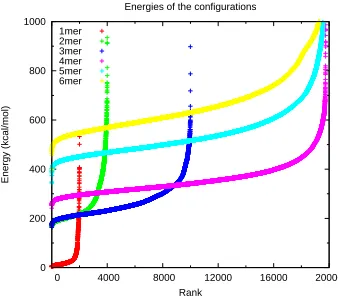
The landscape for the ranking of all the generated structures can be observed in Figure 2.8. We assume there are enough configurations because there is a low enough dip in the beginning of the plot. In other words, there are a few structures with energy lower than the energy of a typical randomly generated structure.
0 200 400 600 800 1000
0 4000 8000 12000 16000 20000
Energy (kcal/mol)
Rank Energies of the configurations
1mer 2mer 3mer 4mer 5mer 6mer
Figure 2.8: Population of all conformers generated for MOCA A to F. Color code: 1mer(A), red; 2mer(B), green; 3mer(C), navy blue; 4mer(D), cyan; 5mer(E), light blue; and 6mer(F), yellow.
In order to determine our best configuration we take the 10 most stable configurations. We can see that we obtain the most stable configuration when we zoom in for the first ranks. In Figure 2.9a and b, we can see that how the configurations for A converges to the most stable ones with 2,000 structures. This is the same case for compound B which the convergence plot can be observed in Figure 2.9c and d for 4,000 structures. For compound C, 10,000 structures were used (Figure 2.9e and f) For compounds D, E and F; 20,000 conformers were used and the convergence curve can be seen in Figure 2.9g-f.
The structures ranked as 1st for each of the compounds are shown in Figure 2.10. Compound A obtained by this method (Figure 2.10a) resembles the one obtained by method I (Figure 2.7a). The main difference is the structure obtained by method II does not have the Fmoc interacting with the O of L-tyrosine. The distance for C-H· · ·O interaction is 5.0 ˚A (compared to 3.6 ˚A from method I). The root mean square (RMS) for the comparison between these two structures is 4.2.
The structure obtained for B is shown in Figure 2.10b. In this structure we do not find any interaction between the Fmoc and the benzene ring of the L-tyrosine or the linkers. There are not hydrogen bonds as in the structure for B found by method I (Figure 2.7b). The Pt+1-Pt+1distances are 22.6 ˚A which is a smaller distance to the one obtained from method I; 28.6 ˚A. When overlapping the structures obtained for B from method I and II, we found that the RMS is 7.86.
Method II gives for Compound C the structure shown in 2.10c. The structure obtained with method II does not show C-H· · ·O Hydrogen bond as the one obtained from Method I (Figure 2.7c). However, there is a very interesting feature found for this structure. The distance between the center Rh to Ru is of only 10.1 ˚A! This is similar to this type of interaction found for compound E and F from method I. Compound C can be defines as the array : Fmoc-(L-tyrosine-Ru)-(L-tyrosine-Pt)-(L-tyrosine-Rh). From our conclusions of method I, we found that the Rh-Ru interaction can be found once the Rh and the Ru are separated by one monomer. We did not find this interaction from method I for compound C but we found such configuration as the most stable from method II. This shows the complementary of both methods to gives a nearly full representation of the important interactions and most stable structures. This suggests that also compound C can have catalytic processes where these two metals can be involved at the same time. The structures for C from the two different methods give similar structures with a RMS of 7.28.
The optimized structure obtained for compound D obtained from method II is shown in Figure 2.10d. Compound D can be described as an Fmoc-(L-tyrosine-Pt1)-(L-tyrosine-Pt2)-(L-tyrosine-Rh)-(L-tyrosine-Ru) sequence. In the most stable structure generated from this method we observe a very interesting interaction between the Rh and Pt1 at a distance 10.3 ˚A. This is the main difference with the structure generated from method I, where such interaction was not found (Figure 2.7d). This also corroborates our postulate that Rh can interact with a second nearest neighbor, and in this case is the monomer with Pt1. The RMS for the overlap of the structures of D obtained from Method I and II is 10.1, which indicates they are not very similar.
Compound E can be represented as follows; Fmoc-(L-tyrosine1-Rh1)-(L-tyrosine2-Pt1)-(L-tyrosi-ne3-Ru)-(L-tyrosine4-Pt2)-(L-tyrosine5-Rh2) and the optimized structure obtained from method I is shown in Figure 2.10e. The Fmoc interacts slightly with the benzene ring from the L-tyrosine binded to Rh1, their separation is about 3.7 ˚A. There are also two hydrogen bonds of nature
N-H· · ·O=C between L-tyrosine1(C=O) and L-tyrosine3(N-H), as well as between L-tyrosine3(C=O)
feature found in this structure is the interaction between Rh1 and Pt1. The separation for this metallic center is 7.1 ˚A, which is the closest interaction we found for any structure. In this interaction of dimers we found a hydrogen bond between the F from the CO2CF3 ligand bounded to Rh1 and the C-H from the pyridine bounded to Pt1. The separation for this C-H· · ·F interaction is 2.9 ˚A with charges for F of -0.32 and for H of +0.17. This kind of interaction in a dimer was already suggested by our QM calculations but it was not observed for the structure E obtained from method I (Figure 2.7e). The RMS for the overlap of the most stable structures obtained from method I and method II is 9.3. This would suggest they are very different however they mostly differ in one dihedral that contains Rh1 and Rh2. This explains why we do not observe the Rh-Ru close interaction but the Rh-Pt interaction with this method.
Compound F is described by the array Fmoc-(L-tyrosine-Pt1)-(L-tyrosine-Rh1)-(L-tyrosine-Pt2)-(L-tyrosine-Ru)-(L-tyrosine-Pt3)-(L-tyrosine-Rh2) and the structure obtained from method II is shown in Figure 2.10f. The main interaction observed for this structure is the presence of the dimer interaction between Pt1 and Rh2. It is the same type of interaction observed for compound E. The Pt1 and Rh2 centers are separated by 7.9 ˚A. There is also a hydrogen bond between the C-H from the pyridine bounded to Pt1 and the F from the CO2CF3 ligand bounded to Rh2. The separation for the C-H· · ·F interaction is 3.1 ˚A with charges for H of +0.18 and for F of -0.32. It is also interesting to note that the adjacent F interacts with the Pt1 center since they are separated by 3.3 ˚
A. The structure from method I and II when overlapped gives a RMS of 16.0 which suggest that these structures are very different.
2.3.3
Conclusions
Compound C have a structure with the Rh-Ru distance of 10.1 ˚A, similar to the distance for this interaction found for compound E and F obtained from Method I. We did not find this interaction from method I for compound C but we found such configuration as the most stable from method II. This also strongly supports our earlier conclusions that Rh(0) is necessary to obtain close distances between metallic centers and if Rh-Ru interaction were to occur, they should be separated by one monomer. Method II also shows for the first time that compound D can present interactions between Rh and Pt. For this type of interaction they do not necessarily need to be second nearest neighbors since the Rh-Pt is not as restricted as the Rh-Ru interaction. This interaction is also observed for compound E and F between Rh and Pt, however we did not observe the Rh-Ru close interactions given by method I for these cases. Our observations show the complementary of both methods, method I observes the Rh-Rh interactions and method II observes the Rh-Pt interactions.
Chapter 3
Coarse-Grained Potential for
Hydrogels from Quantum
Mechanics
Jose L. Mendoza-Cortes, Andres Jaramillo-Botero, William A. Goddard III
3.1
Introduction
Hydrogels are aqueous polymer systems that may exhibit significant strength depending on their composition and structure (e.g. crosslinking). The equilibrium between strength and elasticity makes these materials a potential scaffolding material for cartilage, tendons and ligaments.[21]
There have been many attempts to understand the source of the strength in double network polymer hydrogels at the molecular level, and through the use of atomistic molecular simulations.[22] However, modeling and simulation of important events that occur during the synthesis process, such as percolation, are beyond the capabilities of current atomistic Molecular Dynamics (MD) simulations. To overcome some of these limitations, in particular those associated with the large length and time scales, we proposed the use of a coarse-grained model parameterized from the finer atomistic scale. [23, 24]
Thus, this chapter describes a coarse grained Force Field parameterized from quantum me-chanics (QM) in order to understand the dynamics of polymer hydrogels. The specific polymers described as an example of the parameterization procedure are poly-acrylamide (poly-[aam]) and poly-2-acrylamido-2-2methylpropanesulfonic acid (poly-[amps]).
3.2
Methodology
This section present the methods used from Quantum Mechanics (QM) to calculate the potential energy that can be fitted to a functional form which defines the coarse grained potential.
3.2.1
Molecular Mechanics and Quantum Mechanics
In order to have a good initial guess of the structural features of monomers, dimers, trimers, or even tetramers, we minimized these with the Dreiding force field. [25] The initial guess obtained from molecular mechanics were used to calculate the potential curve of bond breaking and dihedral angles using first principles QM. For this, we used Unrestricted Density Functional Theory (UDFT) with the M06-2X[7] functional as implemented in the Jaguar code[9] and a 6-31G** basis set. All geometries were optimized using the analytic Hessian to confirm that the local minimum had no negative curvature (imaginary frequencies). By studying the transition state we confirm that there is one and only one imaginary frequency.
3.2.2
The Finite Extensible No Linear Elastic (FENE) Potential
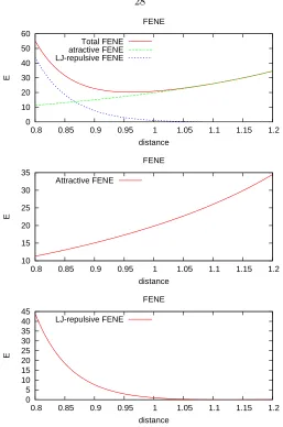
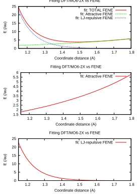
FENE stands for Finite Extensible Nonlinear Elastic. It was initially proposed by Kremer and Grest.[26]
E=−0.5KR02ln
"
1−
r R
![Figure 1.1: Theoretical multiparadigms. (a) was adapted from [1], (b) is courtesy of Julius Su, andPart (c) is courtesy of Andres Jaramillo-Botero.](https://thumb-us.123doks.com/thumbv2/123dok_us/1052545.1131613/24.612.131.520.53.428/figure-theoretical-multiparadigms-adapted-courtesy-julius-courtesy-jaramillo.webp)

![Figure 3.10: [amps-aam] FENE potential for structures in Figure 3.9](https://thumb-us.123doks.com/thumbv2/123dok_us/1052545.1131613/55.612.188.463.332.538/figure-amps-aam-fene-potential-for-structures-figure.webp)
![Table 3.5: [amps-amps] parameters for the FENE potential from QM](https://thumb-us.123doks.com/thumbv2/123dok_us/1052545.1131613/56.612.150.503.192.416/table-amps-amps-parameters-the-fene-potential-from.webp)