Figure 1: Municipalities ordered in decreasing order by the number of words in our corpus (top). Proportion of words (x-axes) occurring in at most the number of municipalities indicated by the y-axes (bottom).
used as a simple way of handling the problem of incomplete data (see examples in Figures 2 and 3).
To find clusters of words with tight distributions in the same regions, those words whose occurrences consist of only one cluster are selected for the second phase. In the second phase the hierarchical clustering algorithm is employed, and the words are clustered with respect to the similarity of the distributions of their occurrences. We defined the distance of two distributions of dialect words as the average of the pairwise distances between the occurrences of the words, that is, dist(w1, w2) = Pk
i=1 Pn
j=1d(mi, m
0
j)/kn.wherew1 andw2 are words,
the municipalities of occurrences being m1, . . . , mk, and
m01, . . . , m0n, respectively, and d(mi, m 0
j) is the distance between the occurrences mi of w1, andm
0
j of w2. Here
we used the Euclidean distances between the occurrences.
The first-phase algorithm can also be employed to find words with geographically isolated regions of occurrences. In that case two occurrences are assigned to the same clus-ter unless there are at leastk >> 0successive
municipal-Figure 2: Example of a tight distribution (ensipoikainen), one skip allowed in the adjacency graph.
Figure 3: Example of a distribution with two geographi-cally isolated distribution areas (aanata’anticipate, fore-see’).
ities without occurrences between them. Then, if several clusters are found, they are isolated from each other. If needed, the resulted occurrences in each region can be fur-ther clustered to evaluate, for instance, whefur-ther they are sufficiently tight for the purposes of the current analysis.
5.
Results
Western dialects
1. South-Western dialects
2. Mid-South-Western dialects
3. Tavastian dialects
4. Southern Ostrobothnian dialects
5. Central and Northern Ostrobothnian dialects
6. Northernmost dialects
Eastern dialects
7. Savonian dialects
8. South-Eastern dialects
Figure 4: Finnish dialects (Savij¨arvi and Yli-Luukko, 1994)
the successive municipalitiesk, l∈ M in the path it holds that eitherk ∈ Ma, orl ∈ Ma (or both). HereM is the set of all the municipalities. In other words, in the path single municipalities with no occurrence are allowed but two successive municipalities with no occurrence are not allowed. Applying these criteria on the corpus resulted in 1012 distributions (6 % of total). An example of a distri-bution satisfying the requirements is given in Figure 2. Of course we also conducted trials with other parameter values with slightly different results. Allowing several skips in a path in the neighbourhood graph rapidly extends the set of distributions.
In the second phase we clustered the selected distributions by the hierarchical clustering algorithm, and stopped the clustering when 100 clusters were left. Most of the clusters consisted of single words. Four of the resulting clusters in-cluded more than 100 words, and 11 of them consisted of more than 20 words. Figures 5 and 6 illustrate the cov-ers of the geographical regions of the largest clustcov-ers. The greater the circle drawn on the municipality, the greater the proportion of the words of the cluster that occur in the mu-nicipality.
For comparison of the results, we also present a division of Finnish dialects into eight regions in Fig. 4, the division
be-ing mainly based on phonological and morphological fea-tures (Savij¨arvi and Yli-Luukko, 1994).
Figure 5: Summary of clustering the tight distributions, West Finland.
The largest cluster in the sense of number of dialect words (237 words, Figure 5, top-left) agrees very closely on the area of Southern Osthrobothnian dialects in Fig. 4. There is a relatively large set of core municipalities that cover remarkable proportions of the dialect words in the clus-ter. Hence, a large set of representative words can be as-signed to the district. The distinctiveness of the Southern Osthrobothnian dialects has been noticed in earlier studies as well. Still, the gradual change of lexicon is indicated by the fact that there are municipalities from dialect regions 3a and 7g that also share part of the word distributions in the cluster.
the distributions but the individual word distributions scat-ter to the Southern Osthrobothnian and Tavastian regions.
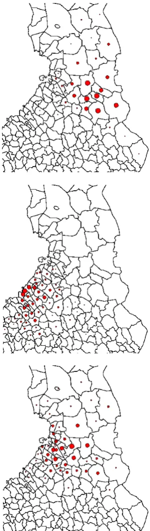
Figure 6: Summary of clustering the tight distributions, East Finland.
The Savonian dialect region is large, and all the clusters summarized in Fig. 6 include word distributions that cover municipalities in the region. The gradual change of lexicon between the regions of Fig. 4 is demonstrated by several of the clusters in Fig. 6. The largest of the clusters (104 words, top-left) settles down in the south-east, the emphasis being on the Tavastian and Savonian dialect regions, only very slightly reaching the southernmost municipalities in the province of Karelia, and the region of the South-Eastern dialects. A kind of counterpart is the centre-left cluster
(58 words) that is located around the town of Lappeen-ranta (area 8c in Fig. 4), and thus, has its geographical emphasis in South Karelia. The bottom-left cluster of 28 words covers municipalities further to the north-east, in the South-Eastern as well as the Savonian regions. The right-side clusters (top: 59 words, centre: 57 words) are located in the Savonian region; the small cluster of 5 words on the bottom-right also reaches the Northern Osthrobothnian re-gion.
The clusters in Fig. 7 include the distributions of 27 (top), 32 (centre), and 15 (bottom) words. The regions are mainly Savonian (top), Central and Northern Osthrobothnian (cen-tre), and Central/Northern Osthrobothnian and Savonian (bottom).
The rest of the words were assigned to clusters of only 1–5 word distributions. The total of 908 words (90 % of all the selected distributions) belonged to the clusters summarized in Figures 5–7.
The small sizes of the clusters in the north and north-east apparently reflect the use of pairwise Euclidean distances when employing the hierarchical clustering algorithm in the second clustering phase. Hence, further experiments with the shortest-path distance measure could reveal more when it comes to the distributions in the north.
In the case of isolated regions of occurrences, the first-phase algorithm could be used to easily find distributions with several geographically distinct areas. For instance, when requiring two separate areas that could not be reached with less than seven steps in the neighbourhood matrix, and with at least three occurrences in both areas, 857 dis-tributions were selected. (An example was given in Fig. 3). Clustering these distributions is apparently much harder than in the case of tight distributions. We clustered each of the distinct subdistributions of a dialect word separately, and, finally, we assigned two wordsw1andw2to the same
cluster, if for each separate set of occurrences of w1, one
of the separate sets of occurrences of w2 belonged to the
same cluster after the second-phase clustering. This prac-tice resulted in some interesting clusters but in general more sophisticated methods should be devised.
6.
Ongoing and future work
Figure 7: Summary of clustering the tight distributions, Central/North Finland.
We are currently modeling the sampling process of the mu-nicipalities and the missing data by Bayesian hierarchical modeling with spatial (Markov random field) dependen-cies, and implementing efficient Markov chain Monte Carlo simulators for estimating the model parameters. The goal is to evaluate whether modifying the data based on the model influences the observed linguistic variation. One of the in-teresting features of such models is the possibility of taking ancillary information, such as known water routes, histor-ical borders etc. into account when modeling the spatial
interaction between areas.
7.
Conclusion
In connection with the project for a comprehensive dic-tionary of Finnish dialects geographical distributions of a large set of dialect words have been stored in electronic form. These 17,126 distributions comprise the corpus stud-ied in this paper. We demonstrate how simple clustering algorithms can be used to extract representative sets of di-alect words for different regions. More complex cluster-ing methods are needed for automatically clustercluster-ing words appearing in two or more areas that are geographically far from each other, and isolated in the sense that there are no occurrences between the areas.
8.
References
S. Embleton and E. S. Wheeler. 1997. Finnish dialect atlas for quantitative studies. Journal of Quantitative Linguis-tic4 (1–3):99–102.
W. Heeringa and J. Nerbonne. 2002. Dialect areas and dialect continua. Language Variation and Change
13:375—398.
S. Hyv¨onen, A. Leino, and M. Salmenkivi. 2006. Mul-tivariate analysis of dialect data. Manuscript submitted
toLiterary and Linguistic Computing(under review
pro-cess).
L. Kettunen. 1940. Suomen murteet III A. Murrekartasto. Suomalaisen Kirjallisuuden Seura.
J. Nerbonne, and W. Kretzschmar 2003. Introducing Com-putational Techniques in Dialectometry. Computers and
the Humanities, 37:245–255.
J. Nerbonne, and P. Kleiweg. 2003. Lexical Distance in LAMSAS. Computers and the Humanities, 37:339–357. A. Leino, S. Hyv¨onen, and M. Salmenkivi. 2006. Mit¨a murteita suomessa onkaan? Murresanaston kvantitati-ivista analyysia.Viritt¨aj¨a, 37:245–255.
M. Palander, L. L. Opas-H¨anninen, and F. Tweedie. 2003. Neighbours or enemies? competing variants causing dif-ferences in transitional dialects. Computers and the
Hu-manities, 37:359—372.
I. Savij¨arvi and E. Yli-Luukko. 1994. J¨ams¨an ¨aij¨an
mur-rekirja. Suomalaisen Kirjallisuuden Seuran
toimituk-sia 618. Suomalaisen Kirjallisuuden Seura.
Tuomi, Tuomo (toim.) 1989. Suomen murteiden sanakirja.
Johdanto. Kotimaisten kielten tutkimuskeskuksen