Term Contributed Boundary Feature using Conditional Random Fields for Chinese Word Segmentation Task

(1)

Term Contributed Boundary Feature using Conditional Random

Fields for Chinese Word Segmentation Task

Tian-Jian Jiang†‡ Shih-Hung Liu*‡ Cheng-Lung Sung*‡ Wen-Lian Hsu†‡ †

Department of Computer Science, National Tsing-Hua University *

Department of Electrical Engineering, National Taiwan University ‡

Institute of Information Science, Academia Sinica

{tmjiang,journey,clsung,hsu}@iis.sinica.edu.tw

Abstract

This paper proposes a novel feature for conditional random field (CRF) model in Chinese

word segmentation system. The system uses a conditional random field as machine learning

model with one simple feature called term contributed boundaries (TCB) in addition to the

“BIEO” character-based label scheme. TCB can be extracted from unlabeled corpora

automatically, and segmentation variations of different domains are expected to be reflected

implicitly. The dataset used in this paper is the closed training task in CIPS-SIGHAN-2010

bakeoff, including simplified and traditional Chinese texts. The experiment result shows that

TCB does improve “BIEO” tagging domain-independently about 1% of the F1 measure

score.

Keywords: Term contributed boundary, Conditional Random fields, Chinese word segmentation.

1. Introduction

Word segmentation is a trivial problem for most Western language, since there are clear

delimiters (e.g. spaces) for individual words. However, for some Asia languages such as

Chinese, Japanese and other language do not have word delimiters, word segmentation

problem will be encountered if we want to do some further language processing, e.g.

information retrieval, summarization and so on. Thus, the Chinese word segmentation could

be viewed as a fundamental problem for natural language processing.

Chinese word segmentation is still a challenging issue, and there is contest held in

SIGHAN community [1]. The CIPS-SIGHAN-2010 bakeoff task of Chinese word

segmentation is focused on cross-domain texts [2]. The design of data set is challenging

particularly. The domain-specific training corpora remain unlabeled, and two of the test

corpora keep domains unknown before releasing, therefore it is not easy to apply ordinary

(2)

(3)

function might be value one when is the state B, is the state I, and is the

character “全”.

1

− t y

max

Y

t

y xt

Given such a model as defined in Eq. 1, the most probable labeling sequence for an input

sequence X is as follow.

)

|

(

arg

*

X

Y

P

y

=

_Λ (2)

Eq. 2 can be efficiently calculated by dynamic programming using Viterbi algorithm. The

more details about concepts of CRF and learning parameters could be refer to [7]. Figure 1

shows the CRF tagging, which is based on BIEO label training, in test phase when given the

un-segmented input.

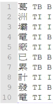
Figure 1. Illustration of CRF prediction

3. Term Contributed Boundary

The word boundary and the word frequency are the standard notions of frequency in

corpus-based natural language processing, but they lack the correct information about the

actual boundary and frequency of a phrase’s occurrence. The distortion of phrase boundaries

and frequencies was first observed in the Vodis Corpus when the bigram “RAIL

ENQUIRIES” and trigram “BRITISH RAIL ENQUIRIES” were examined and reported by

O'Boyle [8]. Both of them occur 73 times, which is a large number for such a small corpus.

“ENQUIRIES” follows “RAIL” with a very high probability when it is preceded by

“BRITISH.” However, when “RAIL” is preceded by words other than “BRITISH,”

“ENQUIRIES” does not occur, but words like “TICKET” or “JOURNEY” may. Thus, the

bigram “RAIL ENQUIRIES” gives a misleading probability that “RAIL” is followed by

“ENQUIRIES” irrespective of what precedes it. This problem happens not only with

word-token corpora but also with corpora in which all the compounds are tagged as units

since overlapping N-grams still appear, therefore corresponding solutions such as Zhang et al.

(4)

We uses suffix array algorithm to calculate exact boundaries of phrase and their

frequencies [10], called term contributed boundaries (TCB) and term contributed frequencies

(TCF), respectively, to analogize similarities and differences with the term frequencies (TF).

For example, in Vodis Corpus, the original TF of the term “RAIL ENQUIRIES” is 73.

However, the actual TCF of “RAIL ENQUIRIES” is 0, since all of the frequency values are

contributed by the term “BRITISH RAIL ENQUIRIES”. In this case, we can see that

‘BRITISH RAIL ENQUIRIES’ is really a more frequent term in the corpus, where “RAIL

ENQUIRIES” is not. Hence the TCB of “BRITISH RAIL ENQUIRIES” is ready for CRF

tagging as “BRITISH/TB RAIL/TI ENQUIRIES/TI,” for example, “TB” means beginning of

the term contributed boundary and “TI” is the other place of term contributed boundary.

In Chinese, similar problems occurred as Lin and Yu reported [14, 15], consider the

following Chinese text:

“自然科學的重要” (the importance of natural science) and

“自然科學的研究是唯一的途徑” (the research on natural science is the only way).

In the above text, there are many string patterns that appear more than once. Some

patterns are listed as follows:

“自然科學” (natural science) and

“自然科學的” (of natural science).

They suggested that it is very unlikely that a random meaningless string will appear

more than once in a corpus. The main idea behind our proposed method is that if a Chinese

string pattern appears two or more times in the text, then it may be useful. However, not all the patterns which appear two or more times are useful. In the above text, the pattern “然科”

has no meaning. Therefore they proposed a method that is divided into two steps. The first

step is to search through all the characters in the corpus to find patterns that appear more than

once. Such patterns are gathered into a database called MayBe, which means these patterns

may be “Chinese Frequent Strings” as they defined. The entries in MayBe consist of strings

and their numbers of occurrences. The second step is to find the net frequency of occurrence

for each entry in the above database. The net frequency of occurrence of an entry is the

number of appearances which do not depend on other super-strings. For example, if the content of a text is “自然科學，自然科學” (natural science, natural science), then the net

frequency of occurrence of “自然科學” is 2, and the net frequency of occurrence of “自然科” is

zero since the string “自然科” is brought about by the string “自然科學.” They exclude the

appearances of patterns which are brought about by others; hence their method is actually

equivalent to the suffix array algorithm we apply for calculating TCB and TCF, and the annotated input string for CRF will be “自/TB 然/TI 科/TI 學/TI”. The Figure 2 demonstrates

(5)

(6)

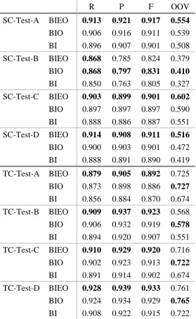
4.2.1 Experiments of Comparison with BI, BIO and BIEO

Experiments here evaluate the performance between three different label schemes “BI”, “BIO”

and “BIEO” for two types (SC and TC) in four domains (Test-A, Test-B, Test-C and Test-D).

The result shows in Table 1. The scheme “BIEO” outperforms “BI” and “BIEO” on F1

measure, except at SC-Test-B. The domain B is computer science and its test data mingles

many English words. In the end of section 4.2.2, we will deal with this problem using

post-processing for English words.

R P F OOV

SC-Test-A BIEO 0.913 0.921 0.917 0.554

BIO 0.906 0.916 0.911 0.539

BI 0.896 0.907 0.901 0.508

SC-Test-B BIEO 0.868 0.785 0.824 0.379

BIO 0.868 0.797 0.831 0.410

BI 0.850 0.763 0.805 0.327

SC-Test-C BIEO 0.903 0.899 0.901 0.602

BIO 0.897 0.897 0.897 0.590

BI 0.888 0.886 0.887 0.551

SC-Test-D BIEO 0.914 0.908 0.911 0.516

BIO 0.900 0.903 0.901 0.472

BI 0.888 0.891 0.890 0.419

TC-Test-A BIEO 0.879 0.905 0.892 0.725

BIO 0.873 0.898 0.886 0.727

BI 0.856 0.884 0.870 0.674

TC-Test-B BIEO 0.909 0.937 0.923 0.568

BIO 0.906 0.932 0.919 0.578

BI 0.894 0.920 0.907 0.551

TC-Test-C BIEO 0.910 0.929 0.920 0.716

BIO 0.902 0.923 0.913 0.722

BI 0.891 0.914 0.902 0.674

TC-Test-D BIEO 0.928 0.939 0.933 0.761

BIO 0.924 0.934 0.929 0.765

BI 0.908 0.922 0.915 0.722

(7)

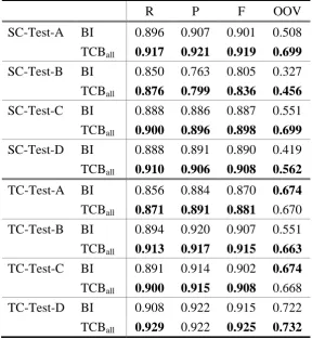
4.2.2 Term Contributed Boundary Experiments with BI as Baseline

In this section, we evaluate the performance of term contributed boundary as a feature in CRF

model training. The label scheme “BI” of ground truth has been treated as baseline for

comparison with TCB features, which label scheme is also “BI”. There are several different

experiments that we have done which are showed in Table 2 and Table 3a and Table 3b. The

configuration is about the trade-off between data sparseness and domain fitness. For the sake

of OOV issue, TCBs from all the training and test corpora are included in the configuration of

results. For potentially better consistency to different types of text, TCBs from the training

corpora and/or test corpora are grouped by corresponding domains of test corpora. Table 2,

Table 3a and Table 3b provide the details, where the baseline is the character-based “BI”

tagging, and others are “BI” with additional different TCB configurations: TCBall stands for

the TCB extracted from all training data and all test data; TCBa, TCBb, TCBta, TCBtb, TCBtc,

TCBtd represents TCB extracted from the training corpus A, B, and the test corpus A, B, C, D,

respectively.

R P F OOV

SC-Test-A BI 0.896 0.907 0.901 0.508

TCBall 0.917 0.921 0.919 0.699

SC-Test-B BI 0.850 0.763 0.805 0.327

TCBall 0.876 0.799 0.836 0.456

SC-Test-C BI 0.888 0.886 0.887 0.551

TCBall 0.900 0.896 0.898 0.699

SC-Test-D BI 0.888 0.891 0.890 0.419

TCBall 0.910 0.906 0.908 0.562

TC-Test-A BI 0.856 0.884 0.870 0.674

TCBall 0.871 0.891 0.881 0.670

TC-Test-B BI 0.894 0.920 0.907 0.551

TCBall 0.913 0.917 0.915 0.663

TC-Test-C BI 0.891 0.914 0.902 0.674

TCBall 0.900 0.915 0.908 0.668

TC-Test-D BI 0.908 0.922 0.915 0.722

TCBall 0.929 0.922 0.925 0.732

(8)

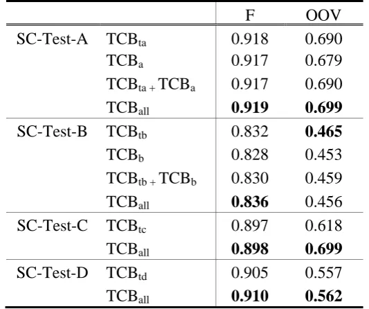
F OOV

SC-Test-A TCBta 0.918 0.690

TCBa 0.917 0.679

TCBta + TCBa 0.917 0.690

TCBall 0.919 0.699

SC-Test-B TCBtb 0.832 0.465

TCBb 0.828 0.453

TCBtb + TCBb 0.830 0.459

TCBall 0.836 0.456

SC-Test-C TCBtc 0.897 0.618

TCBall 0.898 0.699

SC-Test-D TCBtd 0.905 0.557

TCBall 0.910 0.562

Table 3a. Simplified Chinese Domain-specific TCB vs. TCBall

F OOV

TC-Test-A TCBta 0.889 0.706

TCBa 0.888 0.690

TCBta + TCBa 0.889 0.710

TCBall 0.881 0.670

TC-Test-B TCBtb 0.911 0.636

TCBb 0.921 0.696

TCBtb + TCBb 0.912 0.641

TCBall 0.915 0.663

TC-Test-C TCBtc 0.918 0.705

TCBall 0.908 0.668

TC-Test-D TCBtd 0.927 0.717

TCBall 0.925 0.732

Table 3b. Traditional Chinese Domain-specific TCB vs. TCBall

Table 2 indicates that F1 measure scores can be improved by TCB about 1%,

domain-independently. Table 3a and Table 3b give a hint of the major contribution of

(9)

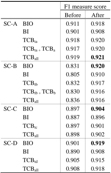
In order to deal with English words, we apply post-processing to the segmented data. It

simply recovers alphanumeric sequences according to their original segments in the training

data. Table 4 shows the experiment result after post-processing. The performance has been

improved, especially on the domain B of computer science, since its data consists of a lot of

technical terms in English.

F1 measure score

Before After

SC-A BIO 0.911 0.918

BI 0.901 0.908

TCBta 0.918 0.920

TCBta + TCBa 0.917 0.920

TCBall 0.919 0.921

SC-B BIO 0.831 0.920

BI 0.805 0.910

TCBtb 0.832 0.917

TCBtb + TCBb 0.830 0.916

TCBall 0.836 0.916

SC-C BIO 0.897 0.904

BI 0.887 0.896

TCBtc 0.897 0.901

TCBall 0.898 0.902

SC-D BIO 0.901 0.919

BI 0.890 0.908

TCBtd 0.905 0.915

TCBall 0.908 0.918

Table 4. F1 scores before and after the English problem fixed

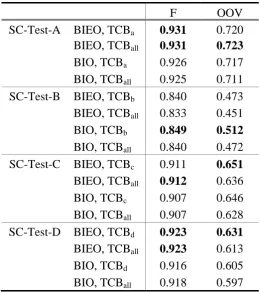
4.2.3 Term Contributed Boundary Experiments with BIO and BIEO

In this section we combine the TCB feature with “BIEO” to compare with “BIO”. Table 5a

and Table 5b show the experimental results. We find that our TCB feature is robustness,

which would not affected by different label scheme. This meets our conjecture, and the

(10)

F OOV SC-Test-A BIEO, TCBa 0.931 0.720

BIEO, TCBall 0.931 0.723

BIO, TCBa 0.926 0.717

BIO, TCBall 0.925 0.711

SC-Test-B BIEO, TCBb 0.840 0.473

BIEO, TCBall 0.833 0.451

BIO, TCBb 0.849 0.512

BIO, TCBall 0.840 0.472

SC-Test-C BIEO, TCBc 0.911 0.651

BIEO, TCBall 0.912 0.636

BIO, TCBc 0.907 0.646

BIO, TCBall 0.907 0.628

SC-Test-D BIEO, TCBd 0.923 0.631

BIEO, TCBall 0.923 0.613

BIO, TCBd 0.916 0.605

BIO, TCBall 0.918 0.597

Table 5a. Simplified Chinese Domain-specific TCB vs. TCBall with BIO and BIEO

F OOV

TC-Test-A BIEO, TCBa 0.909 0.747

BIO, TCBa 0.904 0.744

BIO, TCBall 0.906 0.744

TC-Test-B BIEO, TCBb 0.943 0.771

BIO, TCBb 0.945 0.804

BIO, TCBall 0.945 0.804

TC-Test-C BIEO, TCBc 0.931 0.737

BIO, TCBc 0.928 0.743

BIO, TCBall 0.929 0.745

TC-Test-D BIEO, TCBd 0.942 0.768

BIO, TCBd 0.944 0.778

BIO, TCBall 0.943 0.777

(11)

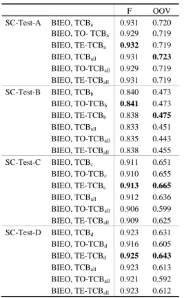
For the sake of consistency, we do extra experiments using label schemes either “BIEO”

or “BIO” to label TCB features, and denote them as TE-TCB and TO-TCB. In these schemes,

“TB,” “TI,” “TE” and “TO” are tags for the head of TCB, the middle of TCB, the tail of TCB,

and the single character word of TCB, respectively. TE-TCB uses all tags but TO-TCB

excludes the tag “TE.” Table 6a and Table 6b show the comparisons between the original

TCB, TO-TCB and TE-TCB. The result suggests that TO-TCB and TE-TCB may not have

stable and significant improvements to the original TCB scheme that consists of only “TB”

and “TI.” We suspect that it is because single character words of TCB and the tail character of

TCB sometimes conflict with the word boundaries of gold standard, after all the concept of

TCB is from suffix pattern, not from linguistic design.

F OOV

SC-Test-A BIEO, TCBa 0.931 0.720

BIEO, TO- TCBa 0.929 0.719

BIEO, TE-TCBa 0.932 0.719

BIEO, TCBall 0.931 0.723

BIEO, TO-TCBall 0.929 0.719

BIEO, TE-TCBall 0.931 0.719

SC-Test-B BIEO, TCBb 0.840 0.473

BIEO, TO-TCBb 0.841 0.473

BIEO, TE-TCBb 0.838 0.475

SC-Test-C BIEO, TCBc 0.911 0.651

BIEO, TO-TCBc 0.910 0.655

BIEO, TE-TCBc 0.913 0.665

SC-Test-D BIEO, TCBd 0.923 0.631

BIEO, TO-TCBd 0.916 0.605

BIEO, TE-TCBd 0.925 0.643

(12)

F OOV TC-Test-A BIEO, TCBa 0.909 0.747

BIEO, TO-TCBa 0.905 0.732

BIEO, TE-TCBa 0.907 0.733

TC-Test-B BIEO, TCBb 0.943 0.771

BIEO, TO-TCBb 0.935 0.734

BIEO, TE-TCBb 0.941 0.759

TC-Test-C BIEO, TCBc 0.931 0.737

BIEO, TO-TCBc 0.930 0.722

BIEO, TE-TCBc 0.931 0.731

BIEO, TE-TCBall 0.932 0.730

TC-Test-D BIEO, TCBd 0.942 0.768

BIEO, TO-TCBd 0.939 0.758

BIEO, TE-TCBd 0.944 0.769

BIEO, TE-TCBall 0.944 0.779

Table 6b. Comparisons between TCB and TX-TCB for Traditional Chinese test set

4.3 Error Analysis

The most significant type of error in our results is unintentionally segmented English words.

Rather than developing another set of tag for English alphabets, we applies post-processing to

fix this problem under the restriction of closed training by using only alphanumeric character

information. Table 4 compares F1 measure score of the Simplified Chinese experiment results

before and after the post-processing.

The major difference between gold standards of the Simplified Chinese corpora and the

Traditional Chinese corpora is about non-Chinese characters. All of the alphanumeric and the

punctuation sequences are separated from Chinese sequences in the Simplified Chinese

(13)

For example, a phrase “服用/simvastatin/（/statins類/的/一/種/）,” where ‘/’ represents the word

boundary, from the domain C of the test data cannot be either recognized by “BIEO” and/or

TCB tagging approaches, or post-processed. This is the reason why Table 4 does not come along

with Traditional Chinese experiment results.

Some errors are due to inconsistencies in the gold standard of non-Chinese character, For

example, in the Traditional Chinese corpora, some percentage digits are separated from their

percentage signs, meanwhile those percentage signs are connected to parentheses right next to

them.

5. Conclusions

This paper introduces a simple CRF feature called term contributed boundaries (TCB) for

Chinese word segmentation. The experiment result shows that it can improve the basic

“BIEO” tagging scheme about 1% of the F1 measure score, domain-independently.

Further tagging scheme for non-Chinese characters are desired for recognizing some

sophisticated gold standard of Chinese word segmentation that concatenates alphanumeric

characters to Chinese characters.

Acknowledgement

The CRF model used in this paper is developed based on CRF++ version

0.49, http://crfpp.sourceforge.net/

The TCBs and TCFs are calculated by YASA (Yet Another Suffix Array) version 0.2.3,

http://yasa.newzilla.org/

6. References

[1] SIGHAN, http://sighan.cs.uchicago.edu/

[2] CIPS-SIGHAN-2010, http://www.cipsc.org.cn/clp2010/

[3] Ma, Wei-Yun and Keh-Jiann Chen, “Introduction to CKIP Chinese Word Segmentation

System for the First International Chinese Word Segmentation Bakeoff,” in Proceedings

of ACL, Second SIGHAN Workshop on Chinese Language Processing, pp. 168–171,

2003.

[4] Lawrence R. Rabiner, “A Tutorial on Hidden Markov Models and Selected Applications

in Speech Recognition,” in Proceedings of the IEEE, Vol. 77, No. 2, pp. 257–286, 1989.

(14)

Information Extraction and Segmentation,” in Proceedings of ICML, 2000.

[6] John Lafferty, Andrew McCallum, and Fernando Pereira, “Conditional Random Fields:

Probabilistic Models for Segmenting and Labeling Sequence Data,” in Proceedings of

ICML, pp. 591–598, 2001.

[7] Hanna M. Wallach, “Conditional Random Fields: An Introduction,” Technical Report

MS-CIS-04-21, Department of Computer and Information Science, University of

Pennsylvania, 2004.

[8] Peter O'Boyle, A Study of an N-Gram Language Model for Speech Recognition, PhD

thesis, Queen's University Belfast, 1993

[9] Ruiqiang Zhang, Genichiro Kikui, and Eiichiro Sumita, “Subword-Based Tagging by

Conditional Random Fields for Chinese Word Segmentation,” in Proceedings of the

Human Language Technology Conference of the NAACL, pp. 193–196, New York, USA,

2006.

[10] Cheng-Lung Sung, Hsu-Chun Yen, and Wen-Lian Hsu, “Compute the Term Contributed

Frequency,” in Proceedings of the 2008 Eighth International Conference on Intelligent

Systems Design and Applications, pp. 325–328, Washington, D.C., USA, 2008.

[11] Fuchun Peng and Andrew McCallum, “Chinese segmentation and new word detection

using conditional random fields,” in Proceedings of Coling-2004, pp. 562–568, Geneva,

Switzerland, 2004

[12] Huihsin Tseng, Pichuan Chang, Galen Andrew, Daniel Jurafsky, and Christopher

Manning, “A Conditional Random Field Word Segmenter for SIGHAN Bakeoff 2005,”

in Proceedings of the Fourth SIGHAN Workshop on Chinese Language Processing, Jeju,

Korea, 2005.

[13] Nianwen Xue and Libin Shen, “Chinese Word Segmentation as LMR Tagging,” in

Proceedings of the Second SIGHAN Workshop on Chinese Language Processing, 2003.

[14]Yih-Jeng Lin and Ming-Shing Yu, “Extracting Chinese Frequent Strings without a

Dictionary from a Chinese Corpus and its Applications,” Journal of Information Science

and Engineering, Vol. 17, pp. 805–824, 2001.

[15] Yih-Jeng Lin and Ming-Shing Yu, “The Properties and Further Applications of Chinese

Frequent Strings,” Computational Linguistics and Chinese Language Processing, Vol. 9,