Predicting discharge at ungauged catchments : parameter estimation through the method of regionalisation

(1)

Predicting discharge

Predicting discharge at ungauged catchments

at ungauged catchments

Parameter estimation through the method of regionalisation

(

Φ

)

=

|

ˆ

R

L

H

θ

(2)

(3)

(4)

- Master Thesis -

Date: 24.11.2006

Title: Predicting discharge at ungauged catchments: Parameter estimation through the method of regionalisation.

Author: D.L.E.H. Deckers

E-mail: [email protected]

Graduation Committee: Dr. M.S. Krol (University of Twente) Dr. ir. M.J. Booij (University of Twente)

(5)

i

I.

Preface

Exactly two and a half years ago I stood for an important decision. After just ending my previous study I had to decide what my next step would be. Making choices is tough. One of the options was to start applying for work. Though, an other interesting option arose by means of an information day at the University of Twente. It persuaded me to enter a new study and my choice was made: Civil Engineering and Management with the differentiation Watermanagement.

Two years went by. But suddenly I stood at the beginning of the end of my second study. At first I tried finding an external assignment since it would hopefully had some practical aspects. However it was not the case. Happily, my current supervisor had posted an interesting research on the intranet and an internal assignment it became. The result lies in front of you.

Half a year I have worked on my master thesis and eventually everything comes to an end. Instead of a more practical side, I can honestly say the assignment turned out to be pretty scientific. Moreover, I can affirm that it has been a very exciting and educational period for me and I would recommend everybody to include such ‘scientific aspects’. Nevertheless, I could not have established this amount of profound research without good advise, motivation and triggering of my supervisors Martijn Booij (UT), Maarten Krol (UT) and Tom Rientjes (ITC). Therefore my well-meant gratitude.

In addition, I would like to thank my girlfriend Daniëlle for her “long-distance” support throughout the week and distraction in the weekends, my parents for total support during the whole study and my fellow students for the pleasant coffee-times, lunch-strolls and many interesting discussions in room number W-122.

Everybody, thanks. Dave Deckers

Acknowledgements

(6)

(7)

iii

II.

Summary

The ability to predict flows at gauged and ungauged catchments is an important goal in hydrology. The reason why prediction is of importance is for instance the ability to estimate impacts of climate or land use change on the discharge regime. For such purposes hydrological models are generally used all over the world. However, in order to be able to predict discharge values for concerning model parameters have to be determined. In general, this is done by calibrating the model against observed discharge using efficiency criteria which evaluate model performance. Yet, with respect to the ungauged catchment topographic and climatic properties are available, but no observed discharge data. Hence, the ungauged catchment can not be calibrated and model parameter values have to be determined using other sources of information. The objective of this study contributing to this issue is as follows: Contribute to reducing uncertainty in the prediction of discharge regime at the ungauged catchments through application of the method of regionalisation based on establishing relationships between model parameters of the hydrological model HBV and climatic and physiographic data using 61 well gauged catchments in the United Kingdom.

The hydrological model HBV is used in this study which can be appointed as a conceptual model. It therefore contains model parameters which not have a direct physical interpretation and hence, model parameter values can not be estimated in the field. The model is run at a time step of one day and requires data on precipitation, actual temperature and potential evapotranspiration in order to be able to simulate discharge. Actual temperature and potential evapotranspiration are calculated using several data sets available at databases from which authorization was requested. For the potential evapotranspiration the formula of Penman-Monteith is applied since it was not directly available. The data sets of precipitation and observed discharge regimes are gathered from another free admissible database.

The classical approach of regionalisation is applied in this study and consists of three steps. The first step implies calibration of the catchments against an observed discharge regime in order to identify model parameter values. Objective functions, which are quantitative measures to estimate model performance, are used to determine the model parameter set which generates the best fit between the observed discharge and the calculated discharge. This is called the optimum parameter set. Secondly, for each selected model parameter it is tried to establish a relationship with climatic and physiographic data. All established relationships together, merged in the hydrological model HBV, are called the regional model. Finally, model parameter values can be estimated by applying the established regional model in order to be able to predict discharge at the ungauged catchment. In this study the performance of the regional model is validated in order to evaluate model performance of the regional model.

With respect to model calibration, at first appropriate model parameters are selected. In this study, the essence is to establish a robust regional model which can adequately predict all the different aspects of the hydrograph such as total average flows, high flows and low flows. Other regionalisation studies, where much experience has been gained are used to select appropriate model parameters. In total 7 model parameters are selected: FC, BETA, LP, ALFA, Kf, Ks and

(8)

iv

values has been a reaction to a commonly known problem in model calibration which is called equifinality. It means that many combinations of parameter values provide equally good model fits to the observed data. Applying a multiple objective function deals with the problem of equifinality. For 48 out of 61 catchments the optimum parameter sets are derived. Regarding the remaining 13 catchments, 8 are used for validating the regional model and 5 are omitted due to different reasons. Based on two conditions, satisfactory catchments are selected to be used for establishing the relationships. The conditions are related to the commonly used Nash-Sutcliffe coefficient (R2_{) and to the relative volume error (}_RV_E_{). In total 17 catchments satisfy both}

conditions.

In order to be able to determine relationships between model parameters and physiographic and climatic data, so called physical catchment characteristics (PCCs) have to be selected. Based on commonly used PCCs in other regionalisation studies and on availability of the required data, in total 14 PCCs are selected which are the catchment area, mean elevation, hypsometric integral, catchment shape, standard average annual rainfall, five types of land use and four types of geology and soils. Subsequently, relationships are established by performing simple and multiple linear regression analysis. In both cases for each model parameter relationships are derived which are evaluated based on statistical and hydrological significance. Also scatter plots between model parameters and PCCs are evaluated since it is assumable that clear non-linear relationships can occur. Eventually for all model parameters significant relationships are derived with the exception of Ks. However, three out of six selected regression equations still are questionable on the basis of

hydrological interpretation.

After having determined the relationships between model parameters and PCCs, the established regional model is validated using the ungauged catchment. In order to be able to draw conclusions regarding model performance well observed discharge data are required and therefore several well gauged catchments are supposed to be ungauged. In order to assess the robustness of the regional model it is assumed that in total 8 well gauged catchments are sufficiently since they are selected based on much physiographic and climatic diversity. Assessing the performance of the regional model is done by comparing it to the performance of the ungauged catchments using the optimum parameter set and using the default parameter set. In this way judgment is made due to change in model performance of the regional model. With respect to model parameter Ks in the

regional model, a default value is used.

After evaluation of model performance of the regional model against the optimum parameter set, it can be concluded that in general the model performs not satisfactorily. At the start of this study it was expected that overall model performance which is represented by R2_{would decrease,}

but within an acceptable range. However, the decrease of R2_{turns out to be considerable for}

(9)

v

III.

Samenvatting

Het voorspellen van afvoer regimes in goed alswel in slecht bemeten stroomgebieden is een belangrijk doel binnen het vakgebied van de hydrologie. Met goed bemeten stroomgebieden worden stroomgebieden bedoeld waar klimatologische data zoals neerslag en temperatuur van beschikbaar is, stroomgebiedbeschrijvende data zoals het gemiddelde verhang en de grootte van het stroomgebied alswel lange termijn data van het gemeten afvoer regime aanwezig is. Reden waarom dit van belang is, is bijvoorbeeld de mogelijk om het effect van klimaatsverandering op het afvoer regime te voorspellen. Hiervoor worden in het algemeen hydrologische modellen gebruikt. Om het voorspellen mogelijk te maken moeten voor betreffende modelparameters waarden worden bepaald. Normaliter worden deze verkregen door het model te kalibreren met de gemeten afvoer regimes. Echter, in slecht bemeten stroomgebieden is deze data niet aanwezig en kunnen derhalve de benodigde parameterwaarden niet worden bepaald waardoor andere bronnen van informatie gebruikt moeten worden. Het doel van dit onderzoek sluit aan bij het laatst genoemde probleem welke is verwoordt als: Draag bij aan het verkleinen van de onzekerheid in het voorspellen van afvoer regime in het slecht bemeten stroomgebied door toepassing regionalisatie welke gebaseerd is op het vaststellen van relaties tussen modelparameters van het hydrologische model HBV en klimatologische alswel stroomgebiedbeschrijvende gebruik makend van 61 goed bemeten stroomgebieden in het Verenigd Koninkrijk.

Het hydrologische model HBV is in deze studie gebruikt wat geclassificeerd wordt als een conceptueel model. Hierdoor bevat het modelparameters die niet directe fysiek geïnterpreteerd kunnen worden en daardoor zijn bijbehorende waarden niet direct in het veld te bepalen. Het model simuleert met een tijdstap van een dag en vereist neerslag, actuele temperatuur en potentiële evapotranspiratie om te kunnen simuleren. De actuele temperatuur en de potentiële evapotranspiratie zijn berekend gebruik makend van verschillende data sets die beschikbaar zijn gemaakt door de British Atmospheric Data Centre. De berekening van de potentiële verdamping is gebaseerd op de formule van Penman-Monteith. De vereiste data sets van waargenomen neerslag en afvoer regime zijn verzameld van een andere vrij toegankelijke data base.

De klassieke aanpak van regionalisatie is in deze studie toegepast en is opgebouwd uit drie stappen. In de eerste stap worden de stroomgebieden gekalibreerd met de gemeten afvoer verlopen om geschikte modelparameter waarden te bepalen. Doelfuncties, welke een kwantitatieve maat zijn om de prestaties van het model te bepalen, worden gebruikt om de optimale parameter set te bepalen. Vervolgens wordt in de tweede stap voor elke modelparameter relaties bepaald met de klimatologische en gebiedsbeschrijvende data. Alle vastgestelde relaties tezamen vormen het regionale model. In de laatste stap worden voor elke modelparameter waarden bepaald in het slecht bemeten stroomgebied gebruik makend van het vastgestelde regionale model. Daarnaast is in deze studie ook het regionale model gevalideerd om een oordeel te geven over de prestaties van het regionale model.

Met betrekking tot de kalibratie van het model zijn allereerst geschikte modelparameters geselecteerd. In deze studie is het de essentie om een robuust regionaal model te bepalen die adequaat alle aspecten van een hydrograaf kan voorspellen zoals het gemiddelde afvoer regime maar ook de piek afvoeren en de laag water afvoeren. Andere regionalisatie studies waar veel evaring is opgedaan zijn geëvalueerd en hierop gebaseerd zijn in deze studie in totaal 7 modelparameters geselecteerd, te weten FC, BETA, ALFA, LP, Kf, Ks en PERC. De optimale

(10)

vi

van een meervoudige doelfunctie is vervolgens bepaald welke van de willekeurig gegenereerde parameter sets de optimale parameter set is. Deze meervoudige doelfunctie is opgebouwd uit vier enkelvoudige doelfuncties die ieder evenredig ten opzichte van elkaar een bepaald aspect van de hydrograaf evalueren. Implementatie van een meervoudige doelfunctie om de optimale parameter set te bepalen is een reactie op een algemeen erkend probleem binnen model kalibratie wat

equifinality wordt genoemd. Dit impliceert dat verschillende combinaties van parameterwaarden

resulteert in even goede model prestaties. Toepassing van een meervoudige doelfunctie pakt het probleem van equifinality aan. Voor 48 van de 61 stroomgebieden zijn uiteindelijk optimale parameter sets bepaald. Van de resterende 13 stroomgebieden zijn er 8 geselecteerd om het regionale model te valideren en zijn er 5 weggelaten om verschillende redenen. Stroomgebieden die na de kalibratie zijn geselecteerd om het regionale model vast te stellen, zijn geselecteerd aan de hand van 2 opgestelde voorwaarden. Deze voorwaarden hebben betrekking op de volgende doelfuncties: de Nash-Sutcliffe coëfficiënt (R2_{) en de relatieve volume fout (}_RV_E_{). In totaal voldoen}

17 stroomgebieden aan deze gestelde twee voorwaarden.

Om überhaupt relaties vast te stellen, moeten er naast de optimale parameterwaarden ook zogenaamde fysieke stroomgebiedkarakteristiek (FSK) geselecteerd zetten. Gebaseerd op frequent gebruikte FSKen in andere regionalisatie studies en op beschikbaarheid van de benodigde data zijn in deze studie 14 FSKen geselecteerd, te weten oppervlakte, gemiddelde hoogte, hypsometrische integraal, vorm van het stroomgebied, gemiddelde jaarlijkse hoeveelheid neerslag, vijf type land gebruik en vier classificaties hydrogeologie. Het daadwerkelijk vaststellen van de relaties is uitgevoerd door enkelvoudige en meervoudige lineaire regressieanalyse. In beide gevallen zijn de relaties geëvalueerd met betrekking tot statistische significantie en vanuit de hydrologische integriteit van de vastgestelde relaties. Daarbij is voor de enkelvoudige lineaire regressieanalyse ook nog een visuele evaluatie van scatter plots tussen modelparameters en FSKen uitgevoerd aangezien het aannemelijk is dat er ook duidelijk niet-lineaire relaties zich voor kunnen doen. Uiteindelijk zijn voor alle modelparameters statistisch significante relaties vastgesteld met de uitzondering van Ks. Echter, de hydrologische integriteit van drie van de zes vastgestelde relaties

worden nog steeds sterk in twijfel getroffen.

Nadat de relaties tussen modelparameters en FSKen zijn vastgesteld, is het regionale model gevalideerd op slecht bemeten stroomgebieden. Om conclusies te kunnen trekken met betrekking tot de prestaties van het regionale model is voldoende goed bemeten afvoer data benodigd en daardoor zijn enkele goed bemeten stroomgebieden als slecht bemeten verondersteld. Om de robuustheid van het regionale model te beoordelen is het aangenomen dat 8 goed gemeten stroomgebieden voldoende zijn aangezien de selectie ervan gebaseerd is op diversiteit in klimatologische data alswel gebiedsbeschrijvende data. Beoordeling van de prestaties van het regionale model is gebaseerd op vergelijking met de model prestaties naar aanleiding van de optimale parameter set en naar aanleiding van een standaard parameter set. Met betrekking tot modelparameter Ks is er in het regionale model een standaard parameterwaarde gebruikt.

Na evaluatie van de prestaties van het regionale model met de optimale parameter set kan geconcludeerd worden dat het regionale model inadequaat presteert. Aan het begin van deze studie werd weliswaar verwacht dat de prestaties zouden afnemen met betrekking tot het regionale model, maar in beperkte mate. De afname blijkt echter behoorlijk te zijn voor bijna alle 8 stroomgebieden kijkend naar de enkelvoudige doelfunctie R2_{. Bovendien, de afname van de andere}

(11)

vii

IV.

2.1. Hydrological processes 5 2.1.1. Hydrological cycle 5 2.1.2. Rainfall-runoff components at catchment scale 6 2.2. Classification of hydrological models 8 2.2.1. Technique of solution 8 2.2.2. Model scale 9 2.3. Model selection 9 2.4. HBV model 10 2.4.1. Precipitation accounting routine 12 2.4.2. Soil moisture routine 12 2.4.3. Quick runoff routine 13 2.4.4. Baseflow routine 14 2.4.5. Transformation function 14 2.4.6. Routing routine 14 2.4.7. Adjustments HBV-model 15 3. Study area and data organization... 17

3.1. Climatic data 17 3.1.1. Precipitation 18 3.1.2. Temperature 19 3.1.3. Potential evapotranspiration 19 3.2. Physiographic data 21 3.2.1. Elevation 21 3.2.2. Catchment size 22 3.2.3. Land use 22 3.2.4. Geology 23 4. Process of regionalisation ... 25

4.1. Introduction 25

4.2. Approach of regionalisation 25

4.2.1. Similarity of spatial proximity 25

4.2.2. Similarity of catchment characteristics 26

4.3. Selection of approach of regionalisation 26

(12)

viii

4.3.2. Problems in model calibration 27

5. Calibration ...29

5.2.2. Selected approach of calibration 31

5.3. Objective function 31

5.3.1. Single objective function 31

5.3.2. Multiple objective function 33

5.4. Methodology Monte Carlo Simulation 33

5.4.1. Composition of multiple objective function 33

5.4.2. Feasible parameter space 34

5.4.3. Number of calibration runs 35

5.4.4. Critical threshold 36

5.4.5. Moving average 36

5.4.6. Initial conditions 37

5.4.7. Calculation of the SOFs 37

5.4.8. Selection conditions for to be used catchments 37

5.5. Model parameter sensitivity 37

6. Establishing the regional model ...39

6.1. Physical catchment characteristics 39

6.1.1. Method of selecting physical catchment characteristics 39

6.1.2. Selected physical catchment characteristics 40

6.2. Regression analysis 43

6.2.1. Concept of regression analysis 43

6.2.2. Significance and strength 45

6.3. Approach of establishing the regional model 46

7. Validation ...49

7.1. Methodology of validation 49

7.1.1. Validation tests 49

7.1.2. Selected validation test 50

7.2. Method of assessing the validated catchments 50

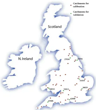
7.3. Catchments for validation 51

7.3.1. Approach of selecting the catchments for validation 51

7.3.2. Selected catchments 52

(13)

ix

8.3.2. Evaluation of the performance of the regional model 74

8.3.3. Additional evaluation of the regional model applied at the calibration catchments 76

8.3.4. Conclusion 79

9. Conclusions, discussion and recommendations ... 81

9.1. Conclusions 81 9.2. Discussion 82 9.3. Recommendations 84 References ... 85

Definitions ... 89

Glossary of abbreviations ... 91

Symbols... 93

Appendices ... 97

A. IAHS, PUB and TDWG... 99

B. Catchments in the study area... 101

C. Calculation potential evapotranspiration ... 103

D. Data assimilation ... 109

E. Evaluating potential evapotranspiration ... 113

F. Values for the required model parameters ... 115

G. Brief description sensitivity model parameters ... 117

H. Benchmarked physical catchment characteristics ... 125

I. Summarized physical catchment characteristics... 127

J. Extended description of relationships ... 129

K. Adjusted parameter space ... 131

L. Optimum parameter set ... 133

(14)

(15)

1 - Introduction

1

1.

Introduction

1.1.

1.1.1.1.

1.1. Scope of the researchScope of the researchScope of the researchScope of the research

The ability to predict flows in ungauged and gauged catchments is an important goal in hydrology. Ungauged catchments here refer to catchments where topographic and climatic properties are available, but no observed discharge data. Reason why prediction at the ungauged and gauged catchment is of importance is for instance:

• the possibility to predict high and low flow regimes, set up by respectively rainfall events and dry spells, to evaluate the consequences on socio-economic level or ecological health of the river system;

• estimating impacts of climate or land use change on the discharge regime.

For these purposes, hydrological models are generally used all over the world (Singh, 1995). Prediction of these discharge regimes in ungauged and gauged catchments brings along a given degree of uncertainty which is reflected in model output. Several underlying aspects as addressed in for instance Hunink (2005) cause this uncertainty, which are:

• Different types of hydrological models which are used as a tool to establish these predictions each have a specific model structure since they represent real world hydrological processes differently.

• Transferring input data from the measurement scale to the model grid scale also introduces uncertainty in model output. The obtained data in the field often has to be aggregated in a way to correspond to the spatial scale required for the hydrological model. Furthermore, the obtained data in the field also has a degree of uncertainty arising from the natural variability these data have.

• The identification of appropriate model parameter values called calibration required for simulating the model also introduces uncertainty in model output.

Minimizing these addressed uncertainties causes predictions to be more accurate and hence, better operational and strategic water management is applicable. Regarding this thesis the main objective concerns the latter cause i.e. reducing the predictive uncertainty associated with identifying appropriate model parameters values.

(16)

1 - Introduction

2

Contribute to reducing predictive uncertainty with respect to discharge regimes in ungauged catchments through application of the method of regionalisation based on establishing relationships between parameters from the hydrological model HBV and physiographic and climatic data from 61 well gauged catchments in the United Kingdom.

determined in the preceding literature study of Deckers (2006), regionalisation will be based on establishing relationships between model parameters and physiographic as well as climatic data.

PUB

Recently, flow prediction in ungauged catchments got more attention, which shows a program launched in 2003 by the International Association of Hydrological Sciences (IAHS) that is aiming to make major research advances, in a coordinated way in this field. This initiative, called Predictions in Ungauged Basins (PUB) aims at “formulating and implementing appropriate science programmes to engage and energize the scientific community, in a coordinated manner, towards achieving major advances in the capacity to make reliable predictions in ungauged basins.” (Sivapalan et al., 2003). The objective of this study associates with this initiative. The Top-Down modelling Working Group (TDWG) within PUB made hydrometric data available of 61 well gauged catchments in the United Kingdom in order to contribute to this aim. For more information about IAHS, PUB and the Top-Down modelling Working Group, see appendix A.

1.2. 1.2. 1.2.

1.2. Objective and research questionsObjective and research questions Objective and research questionsObjective and research questions

The University of Twente is interested in using the data from 61 well gauged catchments in the United Kingdom with respect to the formerly addressed issue i.e. uncertainty in parameter identification. Therefore, the objective of this research is stated as follows:

In order to acquire the knowledge that is needed to fulfil the objective in a structured way several research questions are determined.

Main question

Based on a comparison between calibration and validation results, in what way and how is the performance of the regional model applied in ungauged catchments, which comprehends the established relationships merged in the hydrological model HBV, affected?

Sub-questions

1. What are effective and efficient HBV model parameters to relate to physical catchment characteristics?

2. Which criteria should be used in order to calibrate the HBV model as well as to evaluate the performance of the regional model?

3. Which physical catchment characteristics are available and useable to relate to HBV model parameters?

4. Which statistically significant and hydrologically sensible relationships between the model parameters and physical catchment characteristics can be derived?

(17)

1 - Introduction

3 1.3.

1.3.1.3.

1.3. Outline of the reportOutline of the reportOutline of the reportOutline of the report

(18)

1 - Introduction

(19)

2 - Hydrological modelling

5

2.

Hydrological

Hydrological modelling

modelling

To get insight in hydrological modelling, first insight in hydrological processes is acquired. In paragraph 2.1 the hydrological processes of importance with respect to rainfall-runoff generation are expounded. Furthermore, different aspects concerning hydrological modelling such as the technique of solution and scale issues are described in paragraph 2.2. Subsequently, in paragraph 2.3 selection of the model is expounded which is used in this study. At last, in paragraph 2.4 a brief description of the selected model is given.

2.1. 2.1.2.1.

2.1. Hydrological processesHydrological processesHydrological processesHydrological processes

The processes occurring in and above a catchment, from formation of rainfall to generation of stream flow that leaves the catchment through a river, are many and complex. The most important ones, with respect to rainfall-runoff transformation, are described here. This will lead to a better understanding of the rainfall-runoff processes conceptualized by the HBV model. This is of importance when the hydrologist’s knowledge and expertise is required in assessing model output. 2.1.1.

2.1.1.2.1.1.

2.1.1. Hydrological cycleHydrological cycleHydrological cycleHydrological cycle

The basis of generating rainfall-runoff processes lies in the hydrological cycle. The hydrological cycle can be explained by the interdependence and movement of all forms of water on earth. It usually is described in terms of six major components which are precipitation, infiltration, evaporation, transpiration, surface runoff and groundwater flow. This is shown in figure 2-1. While the driving force of this circulation is derived from the radiant energy received from the sun, evaporation can be stated as the start of the cycle. Therefore, the ocean is the earth’s principal reservoir; it stores over 97 percent of the terrestrial water. Water evaporates into water vapour, where it contributes to clouds formation in the atmosphere. Here it condensates and may give rise to precipitation (e.g. rainfall or snowfall). In the terrestrial portion of the cycle not all of this precipitation reaches the ground surface because some is intercepted by the vegetation cover or by the surfaces of buildings and other structures, and respectively transpires and evaporates back into the atmosphere. The precipitation reaching the ground surface may then collect in order to form

surface runoff, it may infiltrate into the ground or it evaporates back up into the sky (Ward and Robinson, 1990). After infiltration of the precipitation into the soil, the flow process becomes very unpredictable since the catchment runoff behaviour is closely related to the subsurface

(20)

6

physiography, geometry and geology (Rientjes, 2005). This aspect (i.e. these flow processes) is expounded in the following section. In addition, another dominating process arising from catchment precipitation which contributes to rainfall-runoff generation is described.

2.1.2. 2.1.2. 2.1.2.

2.1.2. RainfallRainfall----runoff RainfallRainfallrunoff runoff componentsrunoff componentscomponentscomponents at catchment scale at catchment scale at catchment scale at catchment scale

Catchment precipitation lies on the basis of runoff generating. Through four aggregated flow processes, precipitation can arrive at the outlet point of the catchment. These are through:

• direct precipitation onto the water surface; • overland flow;

• throughflow; • groundwater flow.

These terms are used widely and relatively unambiguously in the literature. However, based on the conditions of the soil which the precipitation bears, the last three flow processes each can embrace several distinctive flow processes. This is outlined below and is illustrated in figure 2-2.

Direct precipitation onto the water surface

Not all of the four addressed flow processes are of equal importance in contributing to the total channel discharge. For example, the contribution of direct precipitation onto the water surface is normally small simply because the perennial channel system occupies only a small percentage of catchment areas. However, where catchments contain a large area of lakes or swamps, open channel precipitation may be persistently important (Ward and Robinson, 1990). This is shown in figure 2-2 by number 8. Furthermore, this flow process is unambiguous.

Overland flow

Precipitation falling on the surface, resulting in a flow of water over the land surface by means of a thin water layer sheet flow is called overland flow. Two types of overland flows can be distinguished based on the conditions of the soil which the precipitation bears. These are the Horton overland flow and the saturation overland flow.

• the Horton overland flow occurs when the intensity of the rainfall is greater than the infiltration capacity of the soil and when the rainfall causes storage of water at the land-surface. This happens when rainfall events are heavy and where mountainous slopes are bare or covered by thin vegetation. This is shown in figure 2-2 by number 1.

• the saturation overland flow occurs when the soil becomes saturated due to the rise of the phreatic groundwater level up to the land surface. Since the infiltration capacity becomes zero, the precipitation cannot infiltrate anymore and will runoff on top of the land surface. It is mostly generated at the bottom part of hill slopes with shallow phreatic groundwater levels. This is shown in figure 2-2 by number 2.

Throughflow

Water that does infiltrate into the soil and then moves laterally through the upper soil horizons towards the stream channel is called throughflow. This throughflow takes place above the phreatic groundwater level. The water above the phreatic groundwater level occurs in two distinct forms, which are in unsaturated form and saturated form. Three types of throughflow can be distinguished, which are the unsaturated subsurface flow, the perched subsurface flow and the macro pore flow.

(21)

7 • Perched subsurface flow occurs where lateral conductivity in the surface horizons of the

soil is substantially greater than the overall vertical hydraulic conductivity through the soil profile. When for instance an impermeable rock layer underlies a top layer, subsurface water will be discharged on top of this rock layer. This is shown in figure 2-2 by number 4.

• Water moving through macro pores and / or small natural pipes is called macro pore flow. Water flow exhibits as ‘free’ flow and, as such, is not controlled by suction head gradients (Rientjes, 2005). It can occur either in the saturated as well as the unsaturated form. This is shown in figure 2-2 by number 5.

Groundwater flow

The groundwater flow is the flow of water in the saturated zone. Since water commonly only moves very slowly through the ground, the outflow of groundwater into the channel may lag behind the occurrence of precipitation by several days, weeks or even years. It tends to be very regular since the saturated zone acts as a large storage zone of percolated water. In general, groundwater flow represents the long-term component of total runoff and is particularly important during dry spells when precipitation, overland flow and throughflow are absent. In addition, the groundwater flow contribution can be rapid or delayed (Ward and Robinson, 1990). These are shown in figure 2-2 respectively by number 6 and 7.

However, persistent misuse of other terms which are outlined here such as quickflow and slowflow respectively direct runoff and baseflow can result in unnecessary confusion. In order to provide consistent terminology, these definitions also are expounded. The terms quickflow and slowflow are commonly used with respect to the hydrograph. The hydrograph represents the runoff generated from a catchment against time. It has to be interpreted as the integral effect of all upstream processes due to rainfall. Under quickflow is understood the sum of channel precipitation, the overland flow and rapid throughflow, and will represent the major runoff contribution during storm periods and most floods. The slowflow on the contrary is the sum of the groundwater runoff and the delayed throughflow. This slowflow can be regarded as continuous flow through often long, dry periods. As can be noticed, a distinction is made between rapid and delayed throughflow. This arises from the fact that there is a variety of possible throughflow

(22)

8

routes, as described earlier. As addressed in Ward and Robinson (1990), part of the macro pore flow and the perched subsurface flow in general contributes to the quickflow. The unsaturated subsurface flow contributes to the slowflow.

2.2. 2.2. 2.2.

2.2. Classification of hydrological modelsClassification of hydrological models Classification of hydrological modelsClassification of hydrological models

Many different types of hydrological models have been developed. Many of these models share structural similarities, because underlying assumptions are the same, but some of the models are distinctly different. In order to gain an overview of the types of model approaches, these are classified on the basis of various characteristics. Underneath, an outline of two classifications is described which are based on the technique of solution and the model scale. It is important to understand the difference between these classes so a suitable hydrological model can be chosen for this study.

2.2.1. 2.2.1. 2.2.1.

2.2.1. Technique of solutionTechnique of solution Technique of solutionTechnique of solution

Based on the technique of solution, Beck (1991) classified the models as metric, conceptual and physically-based. Wheater et al. (1993) expounded this classification and described metric models as models primarily based on observations, seeking to characterize hydrological system response from available time-series in- and output data alone. Besides, these models are based on mathematical equations which do not take into account the underlying physical processes. Conceptual models are described as models seeking to represent all of the hydrological processes perceived to be of importance at the catchment scale input and output relationships. And physically-based models are models representing these hydrological processes in a more classical mathematical-physical form by using numerical solution techniques.

Metric models

As mentioned, metric models are based on mathematical equations that do not take into account physical processes which play a role in the hydrological behaviour of a system. The basis for model calibration is formed by analysis of the model input i.e. precipitation and evapotranspiration and output i.e. observed discharge regime. Metric models typically are always catchment dependent and they are not exchangeable. So, when due to climate or land characteristic change the model does not perform well anymore, it has to be re-calibrated (Rientjes, 2005). An example of such a rainfall-runoff model is the Nash cascade model (Nash, 1957).

Conceptual models

Conceptual models are models using physical catchment characteristics and climatic factors in a simplified manner. The algorithms used in the models structure to simulate flows contain parameters values that often do not have a direct physical interpretation and therefore cannot be measured in the field. Instead, they must be estimated using a calibration procedure whereby the model parameters are adjusted until the natural system output and the model output show an acceptable level of agreement. Because of the fact that the required input and output data are usually easily available, consequently these models are mostly used in rainfall-runoff modelling. The HBV rainfall-runoff model is an example of a conceptual model (Bergström, 1995).

Physically-based models

(23)

2.2.2. Model scaleModel scaleModel scaleModel scale

With respect to model scale, a distinction can be made between spatial and temporal scale. Spatial scale refers to the spatial distribution of the real world characteristics within the hydrological model. Temporal scale refers to the time interval used for the data input and internal computations as well as the interval used for the output and calibration of the model (Singh, 1995).

Spatial scale

Models which treat the catchment as a single unit and use input data, which are believed to be representative at the catchment scale and produce output at a single point, are referred to as lumped models. So, in a lumped model, spatial distribution of the real world characteristics is ignored over the entire model domain and characteristics are represented by averaged values. There are, on the other hand, models that subdivide the catchment into smaller units supposed to be homogeneous in terms of their physical characteristics. Input data are required at this smaller homogeneous scale and the output can also be estimated at different points within the catchment. Such models are referred to as distributed models. After all a middle course is possible, which is called a semi-distributed model. In this model approach the system under study is partitioned in relatively large units that often are selected and bounded by topographic divides within the catchment. Each unit can be considered as a sub-catchment and thus are of various size and commonly are of irregular shape. An important characteristic of this classification is that topographic, physiographic and geologic catchment characteristics as well as meteorological variables are lumped within the scale of the sub-catchment (Rientjes, 2005).

Time scale

The time scale, on which the classification is based, can be defined as a combination of two time-intervals. One of the time intervals is used for input and internal computations. The second is the time interval used for the output and calibration of the model. Resulting from this combination, the models can be classified as continuous based or event based. With respect to the continuous-time based models, different continuous-time steps can be applied such as, hourly, daily, monthly and yearly and its aim is to simulate continuous discharge regimes (Singh, 1995). Event based models on the contrary are applied in order to simulate single runoff events, such as floods with hourly or daily periods or flood seasons as well as dry seasons with daily or monthly periods.

2.3. 2.3.2.3.

2.3. Model selectionModel selectionModel selectionModel selection

(24)

10

Since conceptual models perform at least as well as physically-based models in predicting discharge regimes, and since the required input data are not available at the required discretion, selection of physically-based models is denied. Furthermore, it can be stated that no metric model is chosen since the intention is that a change in climate or land characteristic does not require a re-calibration of the model. The conceptual models on the contrary can be considered as a good compromise between the need for simplicity on the one hand and the need for a firm physical basis on the other hand. This due to the fact that these models are usually able to capture the dominating hydrological processes at the appropriate scale with accompanying formulations (Booij, 2002) and therefore are very suitable when used in the process of regionalisation.

In order to choose the appropriate conceptual model, reference is made to the study of Passchier (1996). Passchier compared between important conceptual hydrological models based on several criteria such as application area, level of complexity and level of detail. The objective of the comparison was to select a model for rainfall-runoff modelling of the Rhine and Meuse catchments based on 4 specific aims which were land use impact modelling, climate change impact modelling, real-time flood forecasting and physically based flood frequency analysis. These aims again were evaluated based on 10 criteria such as reliability, scale and availability. The HBV model together with three other continuous based models performed best. The only criteria on which HBV performed poorly concerned the availability of the model.

Furthermore, the HBV model is used several times with respect to regionalisation (Hundecha and Bárdossy, 2004; Merz and Blöschl, 2004; Seibert, 1999b) and it demonstrated to be a suitable model. Besides, the model is available at the University of Twente and therefore it is selected to be used in this study. The HBV model in its latest version, HBV-96, is expounded in the next section.

2.4. Institute (SMHI) for runoff simulation and hydrological forecasting, but the scope of applications has increased steadily. For instance it has been used for studies about the effects of climate change in Norway and Finland (Bergström, 1995). The model has also been subjected to modifications over time, so more specific situations could be addressed.

Experience has shown however, that the standard version of HBV had some major drawbacks which are outlined in Lindström et al. (1997). Therefore a re-evaluation has been carried out and a new model version has been developed. The HBV-96 model is the final result of this model revision (Lindström et al., 1997). Henceforward when “HBV model” is used, it is referred to the HBV-96 model.

(25)

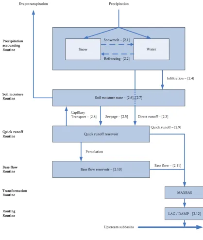
11 Figure 2-3. Schematisation HBV-96 routine structure

The model consists of 6 modules, which are:

• Precipitation accounting routine, representing rainfall, snow accumulation and melt; • Soil moisture routine, representing actual evapotranspiration;

• Quick runoff routine, representing quickflow;

• Baseflow routine, representing slowflow;

• Transformation function, representing quickflow and slowflow delay and attenuation;

• Routing routine, representing flow through river reaches.

(26)

12

parameters to be used can be specified for an individual sub-catchment, or for the catchment as a whole.

2.4.1. 2.4.1. 2.4.1.

2.4.1. Precipitation accountingPrecipitation accounting routinePrecipitation accountingPrecipitation accounting routine routine routine

To simulate rainfall-runoff processes the structure of HBV requires three kinds of data input, which are precipitation, air temperature and estimates of potential evapotranspiration. The time scale of the precipitation is a time step of one day, but if desirable it is possible to set a smaller time step. The evapotranspiration values uses monthly averages, but also smaller values up to the simulation’s time step are possible. The temperature is used for calculations of snow accumulation and melt, but when desired it can be used to adjust the potential evaporation (Lindström et al, 1997; IHMS, 1997). In order to define precipitation as rainfall or snow, a threshold value is used,

TT [0_C_]_._{When temperature,}_T_[o_C_]_,_{becomes smaller than this value, rainfall devolves to snow.}

Interaction between these two components takes place through snowmelt (Ps) and refreezing (Pr),

respectively shown in equation [2-1] and [2-2]:

(

T TT

)

2.4.2. Soil moisture routineSoil moisture routine Soil moisture routineSoil moisture routine

The soil moisture routine is the main part controlling runoff formation. Three output components are generated in this routine, and these are direct runoff, indirect runoff and actual evapotranspiration. Each one of the sub-catchments has an individual soil moisture accounting procedure and response function. Therefore, the runoff is generated independently for each of the sub-catchments.

Direct runoff

The volume of the soil moisture (SM, [mm]) in the catchment is computed with a soil moisture reservoir, representing the unsaturated soil. It uses precipitation (P, [mm/d]) as input which is supplied by the precipitation accounting routine. As long as the maximum soil moisture storage (FC, [mm]) is not exceeded, the precipitation infiltrates into the soil moisture reservoir. Otherwise the precipitation becomes directly available for runoff (DR, [mm/d]) as shown in equation [2-3]:

(

)

The infiltrating water (IN) can be separated into two components; it replenishes the soil moisture state or it will seep through the soil layer, which is parameterized by R [mm/d].

(27)

This relationship between parameters states that indirect discharge increases with increasing soil moisture content and that when no infiltration occurs, no indirect discharge is generated. The amount of water that does not runoff indirectly is added to the soil moisture state.

Evapotranspiration

Actual evapotranspiration (Ea, [mm/d]) which occurs at the soil moisture routine is related to the

measured potential evapotranspiration (Ep, [mm/d]), the soil moisture state and the parameter

value LP [-]. This latter soil moisture value is a fraction between 0 and 1 and denotes the limit where above the evapotranspiration reaches its potential value. This relation is shown in equation [2-6] and [2-7]:

Thus, the actual evapotranspiration is equal to the potential evapotranspiration if the actual evapotranspiration is above the specified threshold.

2.4.3. 2.4.3.2.4.3.

2.4.3. Quick runoff routineQuick runoff routineQuick runoff routineQuick runoff routine

The runoff generation routine is the response function which transforms excess water from the soil moisture zone (DR + R) to runoff. This response function is represented by an upper non-linear and a lower, linear, reservoir. These reservoirs represent respectively the quickflow and slowflow as defined in paragraph 2.1.2. The quick runoff routine manages the upper non-linear reservoir. In this reservoir three components can be distinguished which are; percolation to the slow reservoir, capillary transport back to the soil moisture reservoir and quick runoff.

Percolation

The direct runoff (DR) and indirect runoff (R) together enter the quick runoff reservoir from which a specific amount percolates through to the underlying baseflow runoff reservoir. Percolation (PERC, [mm/d]) only occurs when there is water available in the quick runoff reservoir.

Capillary rise

The second component within the quick runoff reservoir regards water returning to the soil moisture routine. This capillary flow (Cf, [mm/d])depends on the amount of water stored in the

soil moisture reservoir. The parameter CFLUX [mm/d], a maximum value for capillary flow, determines a limitation for the capillary flow. The capillary flow depends on the soil moisture deficit (FC – SM). When there is no soil moisture deficit, no capillary rise will occur. Otherwise, a fraction of the CFLUX will flow capillary upward. This is shown in equation [2-8]:



When the yield from the soil moisture routine is higher than PERC and Cf allows, and water is

available in the quick runoff reservoir, quick runoff (Q0, [mm/d]) is determined through equation

(28)

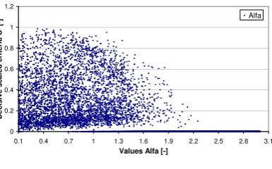
2 - Hydrological modelling linearity of the reservoir and Kf[d-1] a recession coefficient. The recession coefficient is determined

using ALFA and two additional parameters hq [mm/d] and khq [d-1_{] representing respectively a}

high flow rate and a recession coefficient at a corresponding reservoir volume [mm]. This is shown in equation [2-10]:

Both additional parameters are approximated from observation data, but should be determined further during the calibration process (van der Wal, 2001).

2.4.4. 2.4.4. 2.4.4.

2.4.4. Baseflow routineBaseflow routine Baseflow routineBaseflow routine

The baseflow routine is the second part of the response function which transforms excess water acquired from the quick runoff routine. It represents the slowflow of the catchment through Q0

[mm/d]. This is represented by equation [2-11]:

LZ K

Q1= _s⋅ [2-11]

in which the recession coefficient Ks [d-1] is the only parameter to be determined. LZ [mm]

represents the water level in the reservoir. 2.4.5.

2.4.5. 2.4.5.

2.4.5. Transformation functiTransformation functionTransformation functiTransformation functionon on

The total discharge, Q = Q0 + Q1, will be routed separately for each sub-catchment through a

transfer function in order to get a proper shape of the hydrograph. This transfer function is a simple filter technique with a triangular distribution of the weights, according to figure 2-4. The generated runoff of one time step is distributed on the following days using one free parameter (MAXBAS). A value of 1 will distribute the runoff of one day over the same day. A higher value of

MAXBAS will distribute the runoff of one day over a larger period of time. As a result, this will lead to a delay and attenuation in the sub-catchment’s discharge.

2.4.6. 2.4.6. 2.4.6.

2.4.6. Routing routineRouting routine Routing routineRouting routine

With the transformation function, for each sub-catchment discharge runoff will be generated. In the routing routine HBV links the catchments by adding the runoff from accompanying

(29)

15 catchments to the local runoff. The inflow from another sub-catchment is assumed to flow through a river channel from the outlet of the upstream sub-catchment to the outlet of the current sub-catchment where the local runoff is added. Besides plain linkage of the sub-catchments, it is possible to delay and attenuate the water in the river channel by using the parameters LAG and

DAMP. A modified version of the Muskingum equation is used for this computation (Shaw, 1994). In brief, this equation simulates the attenuation of the wave amplitude (concerning the parameter

DAMP) and the travel time (concerning the parameter LAG) of the discharge through the sub-catchment.

By the parameter LAG, the river channel will be subdivided into a number of segments. When this parameter is an integer, each segment will refer to a delay of one day. If DAMP has a value of zero, the outflow from a segment equals the inflow to the same segment during the preceding time step, so that the shape of the hydrograph is not changed. If DAMP is not zero, the shape will be changed, as the outflow from a segment will depend on the inflow during the same time step as well as the inflow and the outflow at the preceding time step. This is shown in equation [2-12].

( 1) 1 ; 1 ;( 1) 2

;

; Q C Q C Q C

Q_out_i = _out _i₋ ⋅ + _in_i⋅ + _in _i₋ ⋅ [2-12]

where i is the current model time step and i-1 the previous model time step. The coefficients C1

and C2 are derived through equations [2-13] and [2-14].

(

DAMP

)

2.4.7. Adjustments HBVAdjustments HBVAdjustments HBVAdjustments HBV----modelmodelmodelmodel

Since the catchments used in this study do no include any sub-catchments, the routing routine is not programmed in the FORTRAN interface. Also the transformation function is not programmed since it is expected that the response time of the runoff within the catchment elapses within a time step of one day. Furthermore Kf is directly determined in the process of calibration, thus equation

(30)

(31)

3 - Study area and data organization

17

3.

Study area and data organization

The United Kingdom contains more than 1200 well gauged catchments and all measurements are well documented in large databases. From these extensive datasets, 61 well gauged catchments are used in this study since required hydrometric data are made available free-of-charge by PUB. The information this dataset includes consists of eleven-year records (i.e. from 01-01-1980 till 31-12-1990) of continuous daily mean streamflow [m3_s-1_{] and daily catchment precipitation [}_mm_{]. In}

addition, because this dataset has undergone extensive analysis as reported in several publications, it is considered to be of substantial utility to PUB participants and hence for this study (Littlewood, 2004). Besides hydrometric data, also data about the characteristics of the catchments are required. This information is derived from the National River Flow Archive website which provides a module called the Catchment Spatial Information (CSI) Pages, from which spatial characteristics for around 1200 gauged catchments can be accessed (CSI, 2006). Each spatial information page features a small map showing the distribution of a given spatial dataset within a specific catchment. However, due to limitations of both datasets only 56 catchments are used in this study. Regarding one catchment, no spatial information is available at the CSI pages. The four other excluded catchments turned out to be sub-catchments of one of the 56 catchments. The remaining catchments are presented in appendix B. Furthermore, regarding the boundaries of the catchments, for England and Wales these are based on regional hydrological boundaries compiled through use of the Integrated Hydrological Digital Terrain Model (IHDTM) from the Centre for Ecology and Hydrology (CEH).

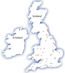
All remaining 56 catchments are situated in England and Wales, thus no catchments are located in Scotland or Northern Ireland. Nevertheless, as can be seen in figure 3-1, they are very well distributed over England and Wales. This contributes to the feasibility of generating a robust regional model due to accompanying variability of climate, topography, geology and land use. The 56 catchments cover 12.398 km2_{of a total of 151.170 km}2_{which corresponds with 8,2% of the}

total area of England and Wales (Encarta, 2006).

3.1. 3.1.3.1.

3.1. Climatic dataClimatic dataClimatic dataClimatic data

(32)

18 3.1.1. 3.1.1. 3.1.1.

3.1.1. PrecipitationPrecipitation PrecipitationPrecipitation

A very substantial advantage for this study is that for each catchment the daily average areal precipitation is available. In the dataset which is made available by PUB, this information is calculated for each catchment based on several observation stations. The number of minimum observation stations used for calculating average areal precipitation varies from 1 to 48. To get insight in the variability of the precipitation across the catchments, the Standard Annual Average Rainfall (SAAR) [mm year-1_{] over the period 1961-1990 is shown in figure 3-2. The minimum}

SAAR holds a value of 566 mm and the maximum SAAR a value of 2055 mm. As can be concluded, moderate dry as well as wet catchments are considered in this study.

0

Figure 3-2. Frequency histogram and cumulative frequency distribution of SAAR

(33)

19 3.1.2.

3.1.2.3.1.2.

3.1.2. TemperatureTemperatureTemperatureTemperature

With respect to actual temperature also average areal temperature for each catchment is required. The dataset provided by PUB however did not include these data. In order to do so authorization is requested at the British Atmospheric Data Centre (BADC, 2006) wherefrom the required data are gathered. The method of acquiring this average areal temperature is described in paragraph 3.1.3. In order to get insight in the variability present across the catchments, the average daily temperature (ADT) is shown in figure 3-3. The minimum ADT across the catchments holds a value of 8.3 0_{C and the maximum ADT a value of 11.0}0_{C. As can be seen, most catchments have an ADT}

between 10.5 0_C_{and 11.0}0_{C. Furthermore, many catchments have an ADT between 9.0}0_C_{and 9.5} 0_{C. After analyzing the spatial distribution of these ADTs it can be concluded that the highest}

ADTs are situated in the southern part of England and the lowest ADTs in the northern part of England. This corresponds with the expected spatial distribution of ADT.

0

3.1.3. Potential evapotranspirationPotential evapotranspirationPotential evapotranspirationPotential evapotranspiration

Third and last necessary data input for running the model is potential evapotranspiration (PE). Just as actual temperature, no PE is included in the dataset provided by PUB. At first the intention was to derive monthly average potential evaporation from general accessible databases from the GeoNetwork opensource Community website (GNOCW, 2006) . However, the best possible spatial resolution the GeoNetwork opensource Community website (GNOCW) hold was 0.5 latitude by 0.5 longitude spacing what corresponds with about 35 kilometre spacing. The combination of spatial and temporal loss regarding the discretion of the data however did decide to improve at least one of both conditions. This since spatial and temporal loss regarding the discretion of precipitation and actual temperature are also reduced to a minimum. Therefore, the database at the British Atmospheric Data Centre (BADC) is used. Although this database does not hold calculated PE for each catchment, many observation stations contain numerous types of information required for calculating PE. Therefore this information is used to calculate the PE using the formula of Penman-Monteith. Strong bases for using this formula are that Penman carried out detailed studies in the United Kingdom in order to construct this formula and that this method is recommended for general use in the United Kingdom by the Meteorological Office (Shaw, 1994). The basic formula for calculating PE is shown in equation [3-1]:

(

)

Figure 3-3. Frequency histogram and cumulative frequency

(34)

20 With:

∆ = slope of the saturation vapour pressure against temperature [kPa 0_C-1_]

γ = hygrometric constant [Pa 0_C-1_]

HT = available energy based on net radiation measurements [mm day-1]

Eat = evaporation and transpiration rate as function of wind speed and saturation deficit

[mm day-1_]

For a complete explanation of this formula, see appendix C.1. In order to determine average areal PE four variables are required: Ta = actual temperature [0C]

ed = saturated vapour pressure at dew point temperature [mm of mercury]

n = bright sunshine [h day-1_]

u2 = wind speed at 2 meter above the surface [miles day-1]

With respect to the temporal scale of the data, at first it is evaluated to use daily observations of the four variables. However, they are not available at the database of the BADC. Since hourly measurements are available, daily averages could be determined. Furthermore, instead of the saturated vapour pressure at dew point temperature, ed, the dew point temperature, Td,is available.

Since these two variables are related, the ed can be calculated from Td and therefore the latter

variable is used. After having decided which variables are used, the method for calculation of the average areal PE regarding the spatial scale is determined.

Since for every catchment the geographical orientation is determined by the location of the discharge observation station and as no other orientation maps are available, the daily average areal PE is gathered based on this known location. Convenience of the multiple search methods of the database of BADC is that it is possible to search for specific data within a certain radius surrounding a given location. Therefore it is chosen to apply this method and use all stations within a certain radius and calculate the mean of accompanying variables.

At first the square root of the catchment area was applied as a search radius, see equation [3-2].

A

r

_a

=

[3.2]

With:

A = area per catchment [km2_]

However, in many cases no observation stations are found and if they were, most of the time the quality of the data is insufficient. Mainly the latter restriction caused that this search criterion was abandoned. Therefore, it is chosen to calculate the mean of the two nearest observation stations with sufficient quality data to determine the values for the variables.

It turned out that not all four variables are measured at the same observation stations. The bright sunshine, n, appeared to be measured solely at other observation stations. In order to gather accompanying values, at first the same search radius is applied. With this search method also no observation stations are found. It appeared that the spatial dispersion of these observation stations was bigger than those of the observation stations with the variables Ta, Tdand u2. After analyzing

(35)

21 After gathered the values for the four variables, the quality of the data is analyzed. Missing and incorrect values are replaced and in what way this is performed, is described in appendix D. Furthermore it is mentioned that the average actual temperature Ta, based on averaging of the two

nearest observation stations, are also solely used as input variable as described in paragraph 3.1.2. In addition an important decision is made with respect to the length of the period to be used for running the HBV model. It turned out that many data for the variables Ta, Tdand u2 were missing

for the first three years (1980 till 1982). Because of these missing values, it is chosen to adjust the period for simulating the model. Instead of starting on 1980, simulation will start on 01-01-1983. Eventually, average areal PE is calculated for each catchment. A detailed description about the determination of the appropriate dataset of the four variables, related issues and the used observation stations for averaging is given in appendix C.2.

In order to get insight in the spatial variability of PE across the catchments, the average annual PE is shown in figure 3-4. The minimum average annual PE holds a value of 569 mm whereas the maximum holds a value of 751 mm. More than 70 % of all catchments have an average annual PE between 625 and 700 mm. Because the PE is calculated, it is preferable to verify the outcome to make sure no mistakes are made during calculation. Therefore the results are visually checked based on datasets derived from the GNOCW with 0.5 latitude and 0.5 longitude spacing. After having generated a map, it was observed that nearly the same values are presented. Also many grid cells hold values between 625 and 700 mm. Furthermore some cells hold values lower than 625 mm but no higher values than 700 mm occurred. Nonetheless, it is assumed that the calculated values are applicable since the values of the GNOCW are long term annual averages from 1961 till 1990. Due to climate change it is assumed that the 8 years used for simulation in this study hold higher values than the average over period of 1961-1990. Therefore, the calculated values which are higher than the long term yearly averages from 1960 till 1990 are representatives of real world PE. For the map used in evaluating the average annual PE, see appendix E.

0

3.2. Physiographic dataPhysiographic dataPhysiographic dataPhysiographic data

3.2.1. 3.2.1.3.2.1.

3.2.1. ElevationElevationElevationElevation

For each of the 56 catchments elevation data are available. These data are derived from the CEH Wallingford Integrated Hydrological Digital Terrain Model (IHDTM). It is based on a 50 m grid

(36)

22

interval (i.e. each cell represents 50 * 50 m2_{) with a 0.1 m vertical resolution. In order to get insight}

in the spatial variability across the catchments, the mean elevation is shown in figure 3-5. The minimum average elevation holds a value of 25.3 meter above sea level (m.a.s.l.) whereas the maximum holds a value of 430.6 m.a.s.l.. Furthermore most catchments have an average elevation between 100 and 200 m.a.s.l. although several catchments do have higher averages. These differences in average elevation of the catchments imply that the 56 catchments are characterized by different topographic structures. The maximum and minimum elevation within catchments supports this implication since the minimum elevation of a specific catchment holds a value of 2.6 m.a.s.l. whereas the maximum holds a value of 1040.0 m.a.s.l..

0

3.2.2. Catchment sizeCatchment size Catchment sizeCatchment size

Also the distribution of the size of the catchments supports the variability. As can be seen in figure 3-6, most of the catchments have a size between 0 km2_{and 150 km}2_{. The smallest catchment holds}

a value of 24.5 km2_{, whereas the largest catchment holds a value of 1480 km}2_.

3.2.3. 3.2.3. 3.2.3.

3.2.3. Land use Land use Land use Land use

Also different land use distributions characterize the catchments, with different catchments having their own predominant land use. At the CSI pages land use maps with corresponding statistics are available which are derived from the Land Cover Map 2000 which is a part of the Countryside Survey 2000. 27 categories are distinguished which are grouped in 7 broader classes. Therefore, some catchments have a predominantly arable cover structure such as the catchments which corresponds to the observation stations 38029 – Quin @ Griggs Bridge and 36003 – Box @ Polstead. Respectively this land use accounts for 78.9% and 75.1% of the catchment area. An other catchment has for instance predominantly mountain cover structure such as the catchment which corresponds to observation station 25006 – Leven @ Leven Bridge. This land use accounts for 63.6% of the catchment area. In general, the most dominating land use present in all the catchments is grassland. The average of this land use holds a value of 42.6% whe