Tiered-Service Fair Queueing (TSFQ): A Practical and Efficient Fair Queueing Algorithm

AMUDALA BHASKER, AJAY BABU. Tiered-Service Fair Queueing (TSFQ): A

Practical and Efficient Fair Queueing Algorithm. (Under the direction of Professor George N. Rouskas.)

A router in today’s Internet has to satisfy two important properties in order to efficiently provide the Quality of Service (QoS) requested by the users. It should be fair among flows and also have low operational complexity. The packet scheduling techniques that have been proposed earlier do not have both these properties. Schedulers like Weighted Fair Queueing (WFQ) provide good fairness among flows but have high operational complex-ity. Schedulers like Weighted Round Robin (WRR) are efficient but provide poor fairness among flows. We propose a new packet scheduling technique, Tiered Service Fair Queueing (TSFQ), which is both fair and efficient. We achieve our goal by applying the concept of traffic quantization. A quantized network offers a small set of service levels (tiers), each with its own weight. Each flow is then mapped to one of the service levels so as to guaran-tee a QoS at least as good as that requested by the flow. We propose different versions of TSFQ, each with its own level of fairness. We present the complexity analysis of the TSFQ scheduler. Finally, we demonstrate through simulations on the TSFQ implementation on

by

AJAY BABU AMUDALA BHASKER

A thesis submitted to the Graduate Faculty of North Carolina State University

in partial fulfillment of the requirements for the Degree of

Master of Science

Computer Science

Raleigh

2006

Approved By:

Dr. Khaled Harfoush Dr. Rudra Dutta

Biography

Ajay Babu Amudala Bhasker was born in Tirupathi and brought up in

Chen-nai, India. After finishing his high school in ChenChen-nai, he graduated with a Bachelor of

Technology (B.Tech) degree in Information Technology from Sri Venkateswara College

of Engineering, University of Madras, Chennai. He joined the department of

Com-puter Science at the North Carolina State University, Raleigh, NC in fall of 2004. He

Acknowledgements

I would like to express my most sincere gratitude to Professor George Rouskas for

having guided me at every step of this research work. This thesis would not have

been possible without his constant support and advice. I am deeply indebted to him

for his patience and invaluable suggestions during the course of this thesis.

I am also thankful to Dr. Rudra Dutta and Dr. Khaled Harfoush for serving on my

thesis committee. I would like to acknowledge the National Science Foundation for

supporting this research.

I would like to thank Zyad Dwekat for all his suggestions throughout this work. I am

grateful to all my friends for their help and support.

Above all, I am grateful to my parents for their love. I am also grateful to my brother,

Contents

List of Figures vi

1 Introduction 1

1.1 Packet Scheduling . . . 1

1.2 Organization of Thesis . . . 2

2 Traffic Quantization: Applications and Algorithms 4 2.1 Traffic Quantization and its Applications . . . 4

2.2 The p-Median Problem . . . 5

2.3 The Directionalp-Median Problem . . . 7

2.3.1 Solutions to the Directionalp-Median Problem . . . 8

2.4 The Constrained Directionalp-Median Problem . . . 10

2.4.1 Solutions to the Constrained Directionalp-Median Problem . . . 11

2.5 Findings . . . 12

3 Generalized Processor Sharing and its Emulations 14 3.1 Generalized Processor Sharing . . . 14

3.2 Weighted Round Robin . . . 16

3.3 Weighted Fair Queueing . . . 18

4 Tiered Service Fair Queueing (TSFQ) 21 4.1 TSFQ for Fixed-Size Packet Traffic . . . 21

4.1.1 Quantization . . . 22

4.1.2 TSFQ Scheduler V.1: One FIFO per Service Level . . . 22

4.1.3 TSFQ Scheduler V.2: TWO FIFOs per Service Level . . . 26

4.1.4 TSFQ Scheduler V.3 . . . 28

4.2 TSFQ for Variable-Size Packet Traffic . . . 31

5 ns Simulations 34 5.1 ns−2 Simulator . . . 34

5.1.1 Packet Scheduling inns−2 . . . 35

6 Numerical Results 40

6.1 Fixed-Size Packets with a Single Service level . . . 42

6.2 Fixed-Size Packets with Multiple Service Levels . . . 44

6.2.1 Small Set of Flows . . . 44

6.2.2 Large Set of Flows . . . 46

6.3 Variable-Size Packets with a Single Service Level . . . 46

6.4 Variable-Size Packets with Multiple Service Levels . . . 55

6.5 Discussion of Findings . . . 60

7 Summary and Future Work 62 7.1 Summary . . . 62

7.2 Future Work . . . 62

List of Figures

2.1 Mapping a set of demand pointsD to a set of supply pointsS in traditional

p-median problem on the real line . . . 6

2.2 Mapping a set of of demand pointsDto a set of supply pointsSin directional p-median problem on the real line . . . 7

2.3 The directional p-median problem with supply points being a multiple of a basic unit r . . . 10

3.1 WRR bursty service for flows A, B, C and D with weights of 0.5, 0.2, 0.2 and 0.1 . . . 17

3.2 WRR smooth service for flows A, B, C and D with weights of 0.5, 0.2, 0.2 and 0.1 . . . 17

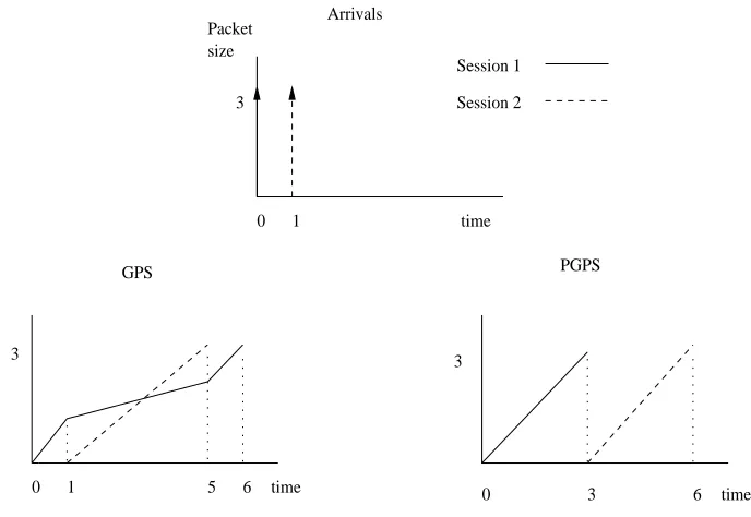
3.3 An example of GPS and PGPS service order of packets from two flows . . . 18

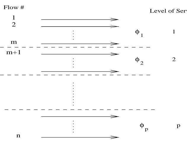
4.1 Quantization of flows: n flows mapped top service levels . . . 22

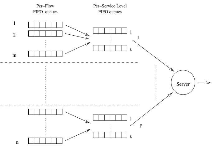
4.2 Structure of the TSFQ Scheduler V.1 . . . 23

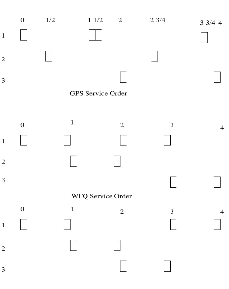
4.3 Fairness Issue Example: Comparison of Servicing Order of GPS, PGPS and TSFQ V.1 . . . 24

4.4 Structure of the TSFQ Scheduler V.2 . . . 27

4.5 Fairness Issue Example: Comparison of Servicing Order of GPS, PGPS and TSFQ V.2 . . . 28

4.6 Structure of the TSFQ Scheduler for Variable-Size Packet Traffic . . . 32

5.1 Composite Construction of a Unidirectional Link inns . . . 35

6.1 Topology used for the simulations . . . 41

6.2 Relative Departure - Single service level, Fixed-size packets - over all flows . 43 6.3 Relative Departure - Single service level, Fixed-size packets - over Flow 1 . 44 6.4 Relative Departure - Single service level, Fixed-size packets - over Flow 2 . 45 6.5 Relative Throughput - Single service level, Fixed-size packets - Flow 1 . . . 46

6.6 Relative Throughput - Single service level, Fixed-size packets - Flow 2 . . . 47

6.8 Relative Departure Multiple service levels, Fixedsize packets 20 flows -over Flow 1 . . . 48 6.9 Relative Departure Multiple service levels, Fixedsize packets 20 flows

-over Flow 2 . . . 48 6.10 Relative Throughput Multiple service levels, Fixedsize packets 20 flows

-Flow 1 . . . 49 6.11 Relative Throughput Multiple service levels, Fixedsize packets 20 flows

-Flow 2 . . . 49 6.12 Relative Departure - Multiple service levels, Fixed-size packets - 1000 flows

- over all flows . . . 50 6.13 Relative Departure - Multiple service levels, Fixed-size packets - 1000 flows

- over Flow 1 . . . 50 6.14 Relative Departure - Multiple service levels, Fixed-size packets - 1000 flows

- over Flow 2 . . . 51 6.15 Relative Throughput - Multiple service levels, Fixed-size packets - 1000 flows

- Flow 1 . . . 51 6.16 Relative Throughput - Multiple service levels, Fixed-size packets - 1000 flows

- Flow 2 . . . 52 6.17 Relative Departure - Single service level, Variable-size packets - over all flows 52 6.18 Relative Departure - Single service level, Variable-size packets - over Flow 1 53 6.19 Relative Departure - Single service level, Variable-size packets - over Flow 2 54 6.20 Relative Throughput Single service level, Variablesize packets 10 flows

-Flow 1 . . . 54 6.21 Relative Throughput Single service level, Variablesize packets 10 flows

-Flow 2 . . . 55 6.22 Relative Departure - Multiple service levels, Variable-size packets - over all

flows . . . 56 6.23 Relative Departure - Multiple service levels, Variable-size packets - over Flow 1 56 6.24 Relative Departure - Multiple service levels, Variable-size packets - over Flow 2 57 6.25 Relative Throughput - Multiple service levels, Variable-size packets - 1000

flows - Flow 1 . . . 57 6.26 Relative Throughput - Multiple service levels, Variable-size packets - 1000

Chapter 1

Introduction

1.1

Packet Scheduling

Technological advances have dramatically increased electronic processing speeds, however so has the transmission capacity of the network links. With the advances in the optical network technologies, the data rate of the network links has increased to 10 Gbps, currently and soon to 40 Gbps. The exponential increase in the amount of bandwidth available within the network has outpaced the improvements in switching and routing ca-pabilities, and this is expected to continue in the future. So, there is a severe mismatch between the bandwidth supported by the network links and the operational speed of the electronic switching and/or routing functions at the network nodes. One such important function of the routing equipment is packet scheduling or queueing.

Packet scheduling refers to the decision process used to select the order in which the packets are transmitted onto the outgoing link. Packet schedulers can be classified into two types:

Work conserving schedulers In these schedulers, the link is never idle when there are packets waiting for service. Most of the existing packet schedulers belong to this type.

Packet scheduling is an important means of controlling congestion and providing specific Quality of Service (QoS) to the flows in the networks. Determining the order in which the packets are serviced is a challenging task because of the QoS requirements of the flows. Each flow in applications such as the World Wide Web (WWW) that involve transfers of data, voice clips and video images have tight bounds on several performance measures such as delay, loss rate, delay jitter, etc. There is also an exponential increase in the number of such flows, making it imperative for the packet scheduler to be very efficient in terms of operational time and also at the same time serve the flows according to their specific QoS requirements.

The goal of this research is to design a practical and efficient packet scheduling scheme. The three important properties of an ideal packet scheduler is as follows:

• Since the schedulers are used in high speed networks, they should have a low opera-tional time complexity, preferably O(1).

• The schedulers should maintain delay bounds for guaranteed-service applications. • The scheduler must provide fairness among the flows competing for the shared link. In

other words, the scheduler must provide fair sharing of bandwidth among the flows. Short-term throughput is a good measure for determining the fairness among the flows.

Few packet scheduling schemes like Weighted Fair Queueing (WFQ) provide good fairness among flows and QoS guarantees, but have relatively high complexity O(log n), where n is the number of flows in the system. Other packet scheduling techniques like Weighted Round Robin (WRR) have an O(1) complexity, but in general do not have good fairness and bounded delay properties.

1.2

Organization of Thesis

Chapter 2

Traffic Quantization: Applications

and Algorithms

In this chapter, we look at the need for applying quantization in packet-switched networks. Also, we look at the p-median problem and the approach to solve the problem of quantization by mapping it to an instance of the p-median problem. We look into the directionalp-median problem, a special case of the traditionalp-median problem, and the solutions to this problem [9]. We then look at an extension to the directional p-median problem and its solution [3]. Finally, we look at the findings made by comparing the quantized networks with the continuous networks [9].

2.1

Traffic Quantization and its Applications

Traffic quantization can be defined as the process of mapping each flow in the network to one of a small set of service levels (tiers), in such a way that a Quality of Service (QoS) at least as good as that requested by the flow is guaranteed. Traffic quantization trades off a small amount of system resources for simplicity in the core network functions, including packet scheduling, traffic policing, etc.

increase in the amount of bandwidth available within a network. Because of this, a router in today’s high speed networks serves hundreds of thousands of flows, each with different QoS requirements. But the ability of routing functions at the network nodes to support per-flow functionality in continuous networks is limited. In a quantized network, per-flow functionality could be supported in an efficient and scalable manner. A quantized network offers a small set of service levels (tiers) and each flow in the network is mapped to one of the tiers, in such a way that a QoS at least as good as requested by the flow is guaran-teed. This simplifies a wide range of network functions. For example, consider the issue of traffic policing. In a continuous-rate network, one flow may request a bandwidth of 99.92 Kbps while another 99.98 Kbps. In this case, the network provider faces a difficult task of distinguishing these two rates and enforcing them reliably. A quantized network might assign both the flows to the next higher level of bandwidth, say 100 Kbps. Now, there is no need for the network provider to distinguish between these two flows. The network operator only needs to supply policing mechanisms for a small set of rates, independent of the number of flows. Traffic quantization may also simplify other network functions such as packet scheduling, traffic engineering, state dissemination, network management, service level agreements, billing, etc.

The disadvantage of a quantized network is that it may consume more resources than a continuous-rate network to satisfy the same set of requests for service. In the case of bandwidth quantization, the total amount of bandwidth required, to service the same set of requests, may be more in a quantized network than in a continuous-rate network. In order to minimize the additional amount of resources, it is important to select an optimal set of service levels. The algorithms presented in the following sections help in determining an optimal set of service levels, given a set of service requests.

2.2

The

p

-Median Problem

d d d d d d d d d d d d d d

s s s s

2 3 4

1

1 2 3 4 5 6 7 8 9 10d11 12 13 14 15

D:

S:

1

0

Figure 2.1: Mapping a set of demand points D to a set of supply points S in traditional

p-median problem on the real line

system by choosing appropriate supply points.

The objective of the p-median problem is to map a set of n demand points D= {d₁, d₂, . . . , d_n} to a set of p supply points S = {s₁, s₂, . . . , s_p} in such a way that the total distance between each demand point and its closest supply point is minimum. In this problem, p is always less than or equal to n and the set of p supply points chosen should be a subset of the ndemand points.

The p-median problem, as a location problem, is usually defined for points on the plane, but can be generalized to points in a k-dimensional system, k ≥ 1. In this work, we will focus on the p-median problem when k = 1, which we will refer to as p-median problem on the real line. Figure 2.1 shows an instance of thep-median problem on the real line where |D |= n= 15 and |S |=p = 4. Down arrows represent demand points, and up arrows represent supply points. This instance is such that demand points d₁−d₃ are mapped to supply points₁, demand pointsd₄−d₇ are mapped to supply points₂, demand points d₈−d₁₂ are mapped to supply point s₃, and demand points d₁₃−d₁₅ are mapped to supply points₄.

Formally, the p-median problem on the real line can be formulated as

M inimize

n

X

i=1

¯

ω(d_i, S) (2.1)

subject to

d₁ ≤d₂≤. . .≤d_N (2.2)

¯

s

1 s2 s3 s4

d d_{1 2} d₃ d d d_{4 5 6} d₇ d d_{8 9} d₁₀d₁₁ d₁₂ d₁₃ d₁₄ d₁₅

D:

S:

1

0

Figure 2.2: Mapping a set of of demand pointsD to a set of supply pointsS in directional

p-median problem on the real line

S⊆D (2.4)

|S|=p (2.5)

d_i∈D (2.6)

1≤p≤n (2.7)

where ¯ω(d_i, S) is the distance between d_i and its nearest supply point.

2.3

The Directional

p

-Median Problem

The directional p-median problem [9] is a special case of the traditional p-median problem. The directional p-median problem on the real line has an additional restriction that the nearest supply point for a given demand point has to be greater than or equal to the demand point itself. Figure 2.2 presents an instance of the directional p-median problem on the real line. The demand set D is identical to that in Figure 2.1, and the number of supply pointsp= 4 as well. However, as we can see, the additional constraint of the directional problem leads to a different solution. For instance, demand points d₁−d₃

sorted in non-decreasing order, find an optimal setS ={s₁, s₂, . . . , s_p} of p supply points, which minimizes the following objective function:

Obj(S) =

p

X

j=1

X

di∈Dj

(s_j−d_i) (2.8)

subject to

S⊆D (2.9)

|S|=p (2.10)

d₁ ≤d₂≤. . .≤d_N (2.11)

s₁≤s₂ ≤. . .≤s_P (2.12)

s_j−1 < d_i≤s_j (2.13)

D_j ⊆D (2.14)

Here, D_j denotes the set of demand points that are mapped to the supply point s_j. Since the problem is directional, all elements in the set D_j are greater than s_j−1 and lesser than or equal tos_j. The sets D₁, D₂, . . . , D_p are exclusive subsets ofD.

An application of the directionalp-median problem is the problem of traffic quan-tization. The QoS requests of the flows and the service levels (tiers) to which they are mapped in a quantized network are analogous to the demand points and supply points, re-spectively, in the directional p-median problem. The directional constraint in the problem assures that the flows receive QoS at least as good as that requested by them. The objective functionObj(S) corresponds to the excess amount of network resources consumed and the goal of the problem is to minimize this excess resource consumption.

2.3.1 Solutions to the Directional p-Median Problem

A simple approach to solve the directional p-median problem is to use the dy-namic programming technique. Given a setD={d₁, d₂, . . . , d_n} of demand points that are sorted in non-decreasing order, the optimal setS ={s₁, s₂, . . . , s_p}can be determined using the following dynamic programming algorithm, as described in [9]. Let the cost function Ψ(R_n, p) denote the minimum cost for mapping all points in setR_ntopsupply points where

Obj(S) = Ψ(R_N, p)−

n

X

i=1

d_i (2.15)

Ψ(R, P) can be computed recursively using:

Ψ(R_n,1) =nd_n, n= 1, . . . , N (2.16) Ψ(R₁, p) =d₁, p= 1, . . . , P (2.17)

Ψ(R_n, p+ 1) = min

q=l,...,n−1{Ψ(Rq, p) + (n−q)dn}, p= 1, . . . , P −1;n= 2, . . . , N (2.18)

This algorithm has an overall time complexity ofO(n2p).

In order to obtain a better complexity bound, [3] used the property of totally monotone matrices and the Monge property to solve this problem. A matrixMhaving real entries is said to bemonotoneifi₁> i₂ implies thatj(i₁)≥j(i₂) wherej(i) is the index of the leftmost column containing the maximum value in row i ofM. Mis said to betotally monotoneif its sub matrices are monotone [2]. The directionalp-median problem can be represented as a Directed Acyclic Graph (DAG), where each arc weight ω(i, k) is the sum of the distances between the demand points d_i+1, d_i+2, . . . , d_k and the demand pointd_k. A complete and weighted DAG satisfies the concave Monge condition if

ω(i, j) +ω(i+ 1, j+ 1)≤ω(i, j+ 1) +ω(i+ 1, j) (2.19) for all 0< i+ 1< j < n. It has been shown that the DAG representing the directional p -median problem obeys the concave Monge condition [9]. Whenn≥m, the Monge property can be used to find the minimum entry in each row or column of a totally monotone

n×m matrix in timeO(n) [2]. The dynamic programming algorithm in (2.16) - (2.18) was modified in [3] to exploit the Monge condition. A new term(i, j) was introduced into the recursive equation, which is defined as the cost of mapping demand pointsd_i+1, d_i+2, . . . , d_k

to point d_k.

(i, k) =

  

0 ifk=i+ 1

(k−i−1)d_k−P_jk₌−1_i+1d_j otherwise (2.20) Now, the dynamic programming algorithm (DPM1 algorithm) is defined as

F(i, j) =

      

0 ifi=j

(j, i) ifj= 1

mini_k−1_=j−1{F(k, j−1) +(k+ 1, i) ifj < i, j 6= 1

s₁ s₂ s₃ s₄ d d_{1 2} d₃ d d d_{4 5 6} d₇ d d_{8 9} d₁₀d₁₁ d₁₂ d₁₃ d₁₄

D:

S:

1 0

d₁₅

r

Figure 2.3: The directionalp-median problem with supply points being a multiple of a basic unit r

Using the DPM1 algorithm to determine the smallest element in each coloumn in totally monotone matrices, we can solve the dynamic programming algorithm in O(np). This is a substantial improvement for problem instances in which the number of demand points (in our case, the number of traffic flows)nis in the order of hundreds of thousands.

2.4

The Constrained Directional

p

-Median Problem

In certain applications, it is necessary to have the solution as a multiple of some basic parameter. For example, data is moved between the main memory and the disk in multiples of the page size. Also in today’s high speed networks, the data transfer rate is usually a multiple of a base rate r. To this end, the directional p-median problem was extended in [3] by adding an additional constraint that all of the supply points are a multiple of some basic unit r. Hence, the new problem of quantization can be defined as follows. Given a set of demand points D = {d₁, d₂, . . . , d_n} find a set of p supply points

S ={s₁, s₂, . . . , s_p}such that the total distance between each demand point and its nearest supply point is minimum and in addition, each supply point should be a multiple of some basic unit r. In other words,

s_i =k_i×r,∀s_i∈S (2.22)

of a basic unit r. The mapping of the demand points to the supply points is identical to that in Figures 2.1 and 2.2, but here, the supply points are multiples of the basic unit r. Considering the Equation (2.22), the objective functionObjective(S) to be minimized will then be

Objective(S) =

p

X

j=1

X

di∈Dj

(r×k_j−d_i) (2.23)

whereD_j is the set of demand points mapped to the supply points_j andr is the basic unit. 2.4.1 Solutions to the Constrained Directional p-Median Problem

Since the p supply points to be selected are multiples ofr, they no longer need to be one of the demand points. So, the algorithm described in the previous section for solving the directional p-median problem was modified to take into account this fact [3]. For each value ofr_i that the basic unitr can take, thepsupply points for the givenndemand points is determined such that all thep supply points are a multiple ofr_i. The objective function

Obj_i(S) for each value is calculated and the optimum r_i that has the minimum objective function is chosen. The problem with this algorithm is that, for each possible value of r

we need to run the DPM1 algorithm which has time complexity of O(np), where n is the number of multiples of r between 0 and 1/p. The total running time of this algorithm is

O(nxp), wherex is the number of possible values ofr. Herenand x are usually very large values. Next, we describe several heuristics for this problem which were first introduced in [3]. The various heuristics trade-off the accuracy with which the minimum objective function is found, for an improvement in the running time.

In the Demand Driven Heuristic (DDH), multiples of r_i that are closest to and greater than the n given demand points are found. These new n points would then be the potential set of supply points, thereby considerably decreasing the time complexity of the algorithm. Even though the total time complexity is still O(nxp), the value of n is comparitively small here.

of r and greater than the p supply points are considered. In Bidirectional Service Driven Heuristic (BSDH), this restriction is not applied. Both the heuristic approaches are faster than DDH by a factor of n, which is a significant improvement for cases where the number of demand points is large.

In the Power of Two Heuristic (PTH), the supply points do not depend on the values of the demand points. The p supply points are always the negative powers of 2 from 20 to 2p−1_{. Obtaining these supply points would take onlyO(p) time and calculating}

the value of of the objective function would take onlyO(n) time. Even though this a fast heuristic compared to others, the amount of resources wasted would be considerably higher when compared to other heuristics.

2.5

Findings

A simulation study conducted by Jackson and Rouskas [9] showed that a small set of service levels is sufficient to approximate the resource usage of a continuous-rate network. In this study, six different distributions were used for generating the demand sets: uniform, triangle, increasing, decreasing, unimodal and bimodal. The results showed that, regardless of the input distribution, the amount of excess resources consumed by quantization decreases sharply as the number of service levelsp increases untilp≈15, beyond which the resource consumption decreases slowly. At this point, the resource consumption is no more than 5-8% resources beyond the amount requested. When the number of demands n increases, the excess resource usage also increases, but the rate of increase is slow. Overall, the results showed that demand sets of 10000 requests can be serviced by 20 or fewer service levels with no more than 5-8% excess resources consumed. Alternatively, we can say that requests up to approximately 92-95% capacity of the link bandwidth can be accepted in a quantized network.

Chapter 3

Generalized Processor Sharing and

its Emulations

In this chapter, we look into the workings of Generalized Processor Sharing (GPS) and the practical scheduling techniques that emulate GPS. There are many scheduling tech-niques that attempt to emulate GPS: Weighted Round Robin (WRR) [5], Deficit Round Robin (DRR) [12], Generalized Virtual Clock (VC) scheduling [13], Self Clocked Fair ing (SCFQ) [6], Weighted Fair Queueing (WFQ) [11], Worst-case Fair Weighted Fair Queue-ing (WF2Q) [4], among others. Out of these emulations, in this chapter we look into the two most popular ones namely, the Weighted Fair Queueing and Weighted Round Robin packet scheduling techniques in detail.

3.1

Generalized Processor Sharing

provides absolute fairness among the users.

GPS is a natural generalization of uniform processor sharing. In uniform processor sharing, all the users are treated equally and they receive the same service. GPS is a work conserving service discipline, since the server is always busy, if there are packets waiting to be served. Letr denote the rate of the server and the positive real numbersφ₁, φ₂, . . . , φ_n

denote the weights of the N different packet flows. LetS_i(t, t+τ) be the service received by flowiat the GPS server in the interval (t, t+τ). If a flowiis continously backlogged in the interval (t, t+τ), then the GPS server satisfies the following condition

S_i(t, t+τ)

S_j(t, t+τ) ≥

φ_i

φ_j, j= 1,2, . . . , N (3.1)

In other words, the service received by the flowirelative to other flows is always greater than or equal to its relative weight. This implies that a flow which is continuously backlogged for some timeτ, will receive service at least as good as it requested, for that time τ. Also, the flowiis guaranteed a rate of

r_i = Pφi

jφj

r (3.2)

The actual rate of service of the flow i(r_i0) is always greater than or equal to r_i. To show this, letB(t) denote the set of backlogged flows at timet. Since the server is work conserving, the rate of service of backlogged flows r_i0 could be higher than the guaranteed rate r_i in an interval (t₁, t₂) in which a set of flows are not backlogged.

r0_i= P φi

j∈B(t)φj

r (3.3)

Since the number of backlogged flows is less than or equal to the total number of flows, i.e.,

B(t)⊆ {1,2, . . . , N}, we have that

X

j∈B(t)

φ_j ≤X

j

φ_j (3.4)

Thus, from equations (2.2), (2.3) and (2.4), we have that

r0_i ≥r_i (3.5)

receive preferential treatment because of the fact that they were idle during the interval (t₁, t₂). GPS scheduler maintains a seperate FIFO queue for each flow sharing the link. Unlike other queueing disciplines like the First Come First Served (FCFS) or the strict priority schemes, GPS does not bound the queueing delay of a packet based on the total queue length on its arrival. Rather it bounds the delay of the packet based on the queue length of the packet’s flow.

GPS provides worst case network queueing delay guarantees and ensures absolute fairness among the flows in the network. Hence, GPS service discipline is the best suited scheme for providing QoS in the networks that serve real time traffic like voice and video. But GPS is an idealized scheme that cannot transmit packets. A GPS server serves all the backlogged flows simultaneously. It also assumes that the traffic is infinitely divisible. In realistic networks, the traffic is made of packets that cannot be broken or divided. Also, a server can provide service to only one flow at any time. An entire packet must be served be-fore another packet can be served. Hence GPS is unimplementable in any realistic network. There are different ways of emulating GPS in networks. Weighted Round Robin (WRR) and Weighted Fair Queueing (WFQ) are two of the most popular ones.

3.2

Weighted Round Robin

Weighted Round Robin (WRR) scheduling discipline is one of the simplest emu-lation of the GPS discipline. WRR is a best-effort scheduling discipline that serves flows based on the weights associated with them. Round Robin scheduling discipline is a special case of WRR where all the flows have equal weights. In Round Robin discipline, the server serves one packet of each backlogged flow in every round. There are two styles of scheduling in WRR - bursty and smooth.

In the bursty service style of WRR scheduling, the server serves a specific number of packets or bytes proportional to the weight of the flow, in every round. (Since it serves a burst of packets from one flow after another, it is called bursty service.) Consider an example of 4 backlogged flowsA,B,C andDwith weights of 0.5, 0.2, 0.2, 0.1 respectively. Then the WRR bursty service order, for every round, would be as shown in Figure 3.1.

A

A

A

A

A

B

B

C

C

D

Figure 3.1: WRR bursty service for flows A, B,C and Dwith weights of 0.5, 0.2, 0.2 and 0.1

A

B

A

C

A

B

A

C

A

D

Figure 3.2: WRR smooth service for flowsA,B,C andDwith weights of 0.5, 0.2, 0.2 and 0.1

flow only once per round. If the flow does not have enough packets to be served in the queue, the server serves fewer number of packets than the allowed number of packets for that flow in that round, even if packets arrive at the queue after the visit by the server. For example, if there are only 2 packets of flowAin the queue, the server serves these 2 packets and moves to the next flow. If a packet of flowAarrives later in that round, the packet has to remain in the queue until the server completes the round and will be transmitted when the server visits the flow in the next round. Hence it also does not provide proper delay guarantees to the packets in the network.

In the smooth service style of WRR scheduling, packets are serviced based on service intervals. The service interval of a flow is inversely proportional to its weight. A flow is serviced only once in a service interval. After the flow is serviced in the interval, it becomes ineligible for service during the remaining time in the interval. Consider the same example of 4 backlogged flowsA,B,C andDwith weights of 0.5, 0.2, 0.2, 0.1 respectively. The service order, for every round, would be as shown in Figure 3.2.

In this style, the jitter is low compared to the bursty service style. But this style has high running time complexity because each time a flow becomes active or inactive, the schedule needs to be recomputed. Even though this style provides better fairness than bursty service style, it still has short-term fairness issues.

3.3

Weighted Fair Queueing

0 1 _{0 3 6}

3

time 3

5 6 time

GPS PGPS

Session 1 Session 2 Arrivals

3

1 time

size

0 Packet

Figure 3.3: An example of GPS and PGPS service order of packets from two flows

Weighted Fair Queueing (WFQ) is the most popular emulation of the GPS. WFQ, also referred to as PGPS (Packet Generalized Processor Sharing), is a packet-by-packet transmission scheme that is a very close approximation of the GPS. Unlike WRR, WFQ works well even when the packets are of variable size.

GPS cannot serve P₂ before P₁, because P₂ does not arrive until time 1. Therefore, the best possible way to emulate GPS is to serve the first packet that would complete service in the GPS, if no additional packets were to arrive after time t. As a result, PGPS serves

P₁ from time 0 to 3 and P₂ from time 3 to 6. P₂ departs the system at time 6, one time unit later than it would depart under GPS. The only packets that are delayed under PGPS are those that arrive late to be transmitted in their GPS order.

WFQ is implemented using virtual time. Virtual time V(t) is used to keep track of the progress of the simulated GPS system. Consider a system with n flows which are associated with n positive real numbers φ₁, φ₂, . . . , φ_n, that denote their weights. Let r

denote the rate of the server. Then, the following expression captures the evolution of virtual time:

V(t_j−1+τ) =V(t_j−1) +P τ

i∈Bjφi

(3.6)

The rate of change of V is

∂V(t+τ)

∂τ =

1

P

i∈B(t)φi

(3.7)

whereB(t) denotes the set of backlogged flows at time t.

Suppose that the kth packet of flow iarrives at time ak_i, and has length Lk_i. Let

S_ik and F_ik denote the virtual times at which this packet begins and completes service, respectively. Letting F_i0 = 0 for all flowsi, we have:

S_ik=max{F_ik−1, V(ak_i)} (3.8)

F_ik=S_ik+L

k i

φ_i (3.9)

The WFQ scheduler serves packets in the increasing order of their virtual finish times F_ik. The main advantages of WFQ are that it is a very close approximation to GPS and it provides excellent worst case network delay guarantees. Let F_p and F_p0 denote the finish times of any packetp in GPS and PGPS respectively. Then,

F_p0−F_p ≤ Lmax

r (3.10)

Chapter 4

Tiered Service Fair Queueing

(TSFQ)

In this chapter, we present how quantization may be applied to packet scheduling in order to overcome the time complexity problem faced by the Weighted Fair Queueing. First, we describe a basic scheduler which is suited only for traffic with fixed-size packets. We also discuss the challenges associated with this new scheduler and the solutions to overcome these challenges. Finally, we present an extension to the design of this basic scheduler that would enable it to work well for traffic with variable size packets.

4.1

TSFQ for Fixed-Size Packet Traffic

1 2

m m+1

n

φ φ

φ

p 2 1

Flow #

Level of Service

1

2

p

Figure 4.1: Quantization of flows: nflows mapped to pservice levels

4.1.1 Quantization

A Tiered Service Fair Queueing (TSFQ) scheduler maps all the flows to service levels (tiers) based on their weights. Consider a quantized network with n flows that are mapped to a small set of p different service levels, as shown in Figure 4.1. Here, p is a constant and p << n. Let ψ₁, ψ₂, . . . , ψ_n, denote the weights associated with the flows. Each service levellhas its own weightφ_l, l= 1,2, . . . , p, and all the flows that are mapped to this service level have the same weight. Each flow is mapped to its closest tier with greater weight. For any flowithat is mapped to a service level l, we have that

φ_l−1< ψ_i ≤φ_l, i= 1,2, . . . , n, l= 1,2, . . . , p

4.1.2 TSFQ Scheduler V.1: One FIFO per Service Level

1 2

m

n

1

p

Server Per−Flow

FIFO queues

Per−Service Level FIFO queues

Figure 4.2: Structure of the TSFQ Scheduler V.1

queues contain the packets, that belong to their respective flows, waiting to be serviced by the scheduler. A packet arriving at a flow queue is inserted at the tail of the queue and therefore the packets within a queue are sorted in the order of their arrival times. The scheduler also maintains one FIFO queue for each service level l,l= 1,2, . . . , p. The FIFO queue at service levellcontains the head-of-line packets of all the backlogged flows that are mapped to this service level.

When a new packet arrives at the head-of-line of the flow queue, it is just added to the tail of the FIFO queue. Consider a packetP arriving at time tthat belongs to flow

i at service level l. The packet could arrive at the head-of-line of flow i’s queue in two situations. The first one is when the packet arrives at an empty flow queue and the second one is when the head-of-line packet of flowi’s queue departs from the system and packetP

1

2

3

4

Time

2

0 3 1/3 5 1/3 6

FLOWS

Service order in GPS

0 1 2 3 4 5 6

1

2

3

4

FLOWS

FLOWS

Service order in TSFQ V.1

0 1 2 3 4 5 6

1

2

3

4

Service order in WFQ

Figure 4.3: Fairness Issue Example: Comparison of Servicing Order of GPS, PGPS and TSFQ V.1

time, it will remain in sorted order after the packet insertion in most cases. We will state an exceptional case later.

queues. This operation involves a comparison of the virtual finish times of p packets, and, given that for a particular system pis a small constant, it takes timeO(1).

There is a fairness issue associated with the one-FIFO per tier scheduler. Figure 4.3 depicts this fairness issue by showing an example of servicing order of packets in GPS, PGPS and TSFQ. In this example, the quantized network has three active flowsf₁, f₂ and

f₃ and one inactive flow f₄ mapped to the same service level l. Also, there are more than one packet in the flow queues off₁, f₂ and f₃ and the time required to service a packet is one time unit. After two packets, one each from flowsf₁andf₂ are served, the FIFO queue would have the new head-of-line packets of these flows at its tail. If the flowf₄, mapped to the same service levell, becomes activated when the scheduler is serving a packet from flow

f₃, this new packet from f₄ would be inserted at the tail of the FIFO queue. This packet from flow f₄ would be served after the packets from flows f₁ and f₂ are served. This is unfair because the virtual finish times of the packets from flowsf₁ and f₂ are greater than the virtual finish time of the packet fromf₄ in the emulated GPS system. The packets from flows f₁ and f₂ start receiving service before its virtual start time. In this example, the service time of the packet fromf₄ is delayed by the sum of service times of the two packets fromf₁ andf₂. In the worst case, the service time of a packet in a TSFQ scheduler can be delayed from its virtual finish time by as much as the sum ofn−2 packets’ service times, wheren is the total number of flows associated with the scheduler.

Let us analyze the worst-case delay performance of this first version of TSFQ. A class of generalized Guaranteed Rate (GR) scheduling algorithms that includes work con-serving algorithms like generalized Virtual Clock, Packet-by-Packet Generalized Processor Sharing (PGPS) and Self Clocked Fair Queueing (SCFQ) algorithms, was defined in [7]. The class of guaranteed rate scheduling algorithms was defined to include algorithms that guarantee that a packet would be transmitted by its guaranteed rate clock (or deadline) value plus some constant. To define the guaranteed rate clock (GRC) value, letpj_f and lj_f

denote thejth packet of flowf and its length, respectively, and letrj,i_f be the rate allocated to packet pj_f at server i. Also, let Ai(pj_f) denote the arrival time of packet pj_f at server i. Then, the guaranteed rate clock value of pj_f at serveri, denoted byGRCi(pj_f, rj,i_f ), is given as:

GRCi(pj_f, rj,i_f ) =max(Ai(pj_f), GRCi(pj_f−1, rj_f−1,i)) + l

j f

whereGRCi(p0_f, r_f0,i) = 0. LetLi_SA(pj_f) denote the departure time of the packetpj_f at server

iusing the scheduling algorithmSA. Then, we can formally state that if

Li_SA(pj_f)≤GRCi(pj_f, rj,i_f ) +βi, (4.2) then the scheduling algorithm SA ∈ GR class. Here, βi _{is a constant denoting the worst}

case delay. GPS is an ideal and unimplementable system with constant factorβi = 0. As we have shown in Section 3.3, WFQ, in the worst case, will delay a packet’s departure from its GRC value by the service time of the maximum sized packet at server i. WFQ also belongs to GR class, with βi = limax

Ci , where Ci is the capacity of the server. Previously

in this section, we showed that this version of TSFQ, in the worst case, will delay the departure of a packet from its GRC value by as much as the sum of n−2 packets’ service time, wherenis the total number of flows associated with the server. Regardless of the fact that the constantβi value of TSFQ is higher compared to WFQ, this first version of TSFQ also provides delay guarantee for all the packets flowing through the scheduler and hence it belongs to the Guaranteed Rate (GR) class. Formally,

Li_{T SF Q}(pj_f)≤GRCi(pj_f, rj,i_f ) +

n−2

X

k=1

l_kmax

Ci (4.3)

wherel_kmax is the maximum length for packets in flowk.

4.1.3 TSFQ Scheduler V.2: TWO FIFOs per Service Level

1 2

m

n

Server Per−Flow

FIFO queues

Per−Service Level FIFO queues

p 1

active FIFO active FIFO inactive FIFO

inactive FIFO

Figure 4.4: Structure of the TSFQ Scheduler V.2

the packets do not start receiving service before their virtual start time, thereby overcoming the fairness problem of the TSFQ V.1 scheduler.

Even though the two-FIFO scheduler solves the fairness problem faced by the one-FIFO scheduler, the addition of another FIFO introduces a new fairness problem. To understand this, consider a system of 3 flows,f₁,f₂ andf₃, assigned to a tierl, as shown in the Figure 4.5. Let us assume that it takes one unit time to service a packet. At time 0, let us assume that the active FIFO queue has one packet from flowf₁ and this packet is being serviced by the scheduler. Also let us assume that the inactive FIFO queue is empty. If at time 1/2 a packet from flow f₂ arrives at the scheduler, it would be added to the tail of the active FIFO. When the packet from flowf₁ finishes its service at time 1, the next packet in its flow queue will be added to the inactive FIFO. If a new packet from flowf₃ arrives just before the departure of the packet fromf₂, it will be added to the tail of the active FIFO. Then, this new packet will be served immediately after the packet from f₂ and before the packet fromf₁, which is in the inactive FIFO queue. But, we can see from the figure that GPS services the packet from f₁ before the packet fromf₃.

1

1 _{2 3}

4

2 3 4

1 1/2 2 2 3/4 _{3 3/4 4} 1/2

GPS Service Order

TSFQ V.2 Service Order WFQ Service Order 3

1

2

3

2 1 2 1

3 0 0

0

Figure 4.5: Fairness Issue Example: Comparison of Servicing Order of GPS, PGPS and TSFQ V.2

The Departureprocedure defines the steps involved in the departure of a packet.

4.1.4 TSFQ Scheduler V.3

Algorithm 1 Arrival(pkt) fid ⇐ flow id of arriving pkt tierid ⇐ tier id of arriving pkt calculate virtual finish time of pkt

if flow queue[fid] is emptythen

if fid is marked inactivethen

insert pkt into the tail of active tier queue[tierid]

else

insert pkt into the tail of inactive tier queue[tierid]

end if

else

insert pkt into the tail of flow queue[fid]

Algorithm 2 Departure

pkt ⇐ packet with minimum virtual finish time in the k active tier queues fid ⇐ flowid of pkt

tierid ⇐ tierid of pkt

if flow queue[fid] is not emptythen

new pkt⇐ head-of-line packet of flow queue[fid]

insert new pkt into the tail of inactive tier queue[tierid]

else

mark fid as active

end if

if tier queue[tierid] is emptythen

mark all flows belonging to tierid as inactive

swap active and inactive tier queue[tierid]

end if

the flow queue of the departed packet is not added immediately to the tail of FIFO during the departure event. It is rather added only when the packet departs in the emulated GPS system. An event is scheduled at the virtual finish time in the head-of-line element of the GPS queue. When this event is dispatched, the head-of-line value of the GPS queue is removed and the virtual finish time of next packet in the flow queue, if any, is added to the tail of GPS queue and the next event scheduled. Also at this point, we add the next packet in the flow queue, if any, to the tail of the FIFO queue. From equation 3.8, we can say that the packets are inserted into the FIFO queue only at their virtual start time.

Lemma 1 Out of all currently available packets, TSFQ V.3 scheduler always serves the

one with the least virtual finish time.

Proof: In TSFQ V.3 scheduler, packets are inserted at the tail of the FIFO queue at their

virtual start time. So, the packets are arranged with in the FIFO queue in the order of

their virtual start time and are also served in the order of virtual start time with in a single

service level. Since the packets within a single service level FIFO have same weights and

same packet size, we can conclude from equation 3.9 that the packets are also served in

the order of their virtual finish time within the service level. Since the scheduler picks the

packet with the least virtual finish time among the head-of-line packets of all the service

level FIFOs, for service, we can conclude that TSFQ V.3 scheduler serves the packet with

the least virtual finish time among all the currently available packets. 2

4.2

TSFQ for Variable-Size Packet Traffic

1 2

m

n

Server Per−Flow

FIFO queues

Per−Service Level FIFO queues

1

p

k 1

k

1

Figure 4.6: Structure of the TSFQ Scheduler for Variable-Size Packet Traffic

for a total ofpk FIFO queues, wherekis a small constant based on the number of common packet sizes. Some of thek FIFOs within a level are used for packets with common packet sizes like 40, 576, 1500 bytes, etc. The remaining FIFOs are used for the packets with sizes between these common values. For example, one queue for packets of size less than 40, another for size 41-575 bytes, another for size 577-1499 bytes and another for packets of size greater than 1500 bytes. In this case, k = 7. For a two-FIFO scheduler, we require two FIFOs for each set of packet sizes within each service level. So, there will be 2kFIFO queues for each service level, for a total of 2pk FIFO queues.

Chapter 5

ns

Simulations

In this chapter, we turn our attention to the implementation details of the dif-ferent scheduler versions proposed in the previous chapter. The schedulers were either implemented or modified in the Network Simulatorns−2. We start with a brief introduc-tion to the simulatorns−2 and then we deal with the implementation of the schedulers in

ns−2.

5.1

ns

−

2

Simulator

ns is a discrete event simulator, developed at the Lawrence Berkeley Labaratory (LBL) of the University of California, Berkeley (UCB) and extended and distributed by the VINT project (a collaboration between University of Southern California (USC)/Information Sciences Institute (ISI), LBL/UCB and Xerox PARC).nsis targeted mainly at networking research and education. ns is widely used by the networking community and is widely regarded as a critical component of research infrastructure. nsprovides substantial support for simulation of TCP, routing, and multicast protocols over wired and wireless (local and satellite) networks.

drophead_ head_

queue_ link_ ttl_

Figure 5.1: Composite Construction of a Unidirectional Link inns

detailed simulations of protocols requires a systems programming language which can ef-ficiently manipulate bytes, packet headers, and implement algorithms that run over large data sets. For these tasks run-time speed is important and turn-around time (run simu-lation, find bug, fix bug, recompile, re-run) is less important. On the other hand, a large part of network research involves slightly varying parameters or configurations, or quickly exploring a number of scenarios. In these cases, iteration time (changing the model and re-running the simulation) is more important. Since configuration runs once (at the beginning of the simulation), run-time of this part of the task is less important. The combination of C++ and OTcl meets both of these needs. C++ is fast to run but slower to change, making it ideal for detailed protocol implementation. OTcl runs much slower but can be changed very quickly (and interactively), making it ideal for simulation configuration. TclCL (Tcl with classes) provides a layer of C++ glue over OTcl, making objects and variables appear in both languages.

5.1.1 Packet Scheduling in ns−2

Inns, a simple link is built from a sequence of connectors. A connector will receive a packet, perform some function, and deliver the packet to its neighbour, or drop the packet.

ns provides the instance proceduresimplex−link to create a unidirectional link from one node to another. The syntax for creating a simplex link is:

$nssimplex−link{f rom−node}{to−node}{bandwidth}{delay}{queue−type}

This command creates a simplex link from node< f rom−node > to node< to−node >

a queue of type < queue−type > is installed for the link. As shown in Figure 5.1, five instance-variables/connectors define a simple unidirectional link:

head Entry point to the link, it points to the first object in the link;

queue Reference to the main queue element of the link;

link Reference to the element that actually models the link, in terms of the delay and bandwidth characteristics of the link;

ttl Reference to the element that manipulates the ttl (time to live) in every packet;

drophead Reference to an object that is the head of a queue of elements that process link drops.

Out of these five instance variables, the queue component is the object of interest to us.

ns currently supports drop-tail (FIFO) queueing, RED buffer management, Class Based Queueing (CBQ), and variants of Fair Queueing including, Fair Queueing (FQ), Stochastic Fair Queueing (SFQ), and Deficit Round-Robin (DRR). Other Scheduling dis-ciplines like Weighted Fair Queueing (WFQ), RED In/Out(RIO) and Core-Stateless Fair Queueing (CSFQ) are available as seperate modules in the Internet. TheQueueclass is the base class of all the queues inns. This class is used by particular types of (derived) queue classes. The class includes two important member functions: enque anddeque. Both these functions are pure virtual, indicating that the particular queues derived fromQueue must implement these two functions. Other member functions are usually not overridden in the derived class.

to send the next scheduled packet downstream (and leave the queue blocked). If there is no packet ready to be sent in the queue, the queue is unblocked.

5.2

TSFQ Implementation in

ns

−

2

To test the performance of the TSFQ schedulers, both the versions were imple-mented in the network simulatorns−2. Since the objective of designing the TSFQ scheduler was to create a scheduler with fairness as good as that of WFQ and running time complex-ity as good as that of WRR, we chose WRR and WFQ for comparing the performance of TSFQ scheduler. ns−2 package includes a Smooth service sytled Weighted Round Robin (SRR) implementation. WFQ implementation for ns−2, contributed by Paolo Losi [1], is available as a separate patch in the ns website. This implementation of WFQ has an infinite queue size and the scheduler never drops a packet. To avoid this, the source code of WFQ implementation was modified to limit the size of the queue. In this modified version of WFQ, the shared buffer size of the queue can be limited in terms of either packets or bytes. One flow may overwhelm the entire queue by sending packets at a high rate. This will affect the other flows since their packets will be dropped when the shared buffer size exceeds the limit. To overcome this problem, each flow is assigned a separate limit based on their weight. When the queue limit is exceeded, only the packets belonging to the flow that has exceeded its own limit is dropped.

TSFQ and TSFQAggregClassifier are the two important classes that define the functioning of the TSFQ. TSFQ class, derived from the base class Queue, is the main queue class of the TSFQ implementation. A TSFQ object is instantiated when a TSFQ queue is defined on a link connecting two nodes. Every TSFQ object defined in the network is associated with a TSFQAggregClassifier object. TSFQAggregClassifier object holds the necessary details for the functioning of the queue. It holds the following details of a TSFQ object:

• The weights associated with the queues (flow-queues) defined within the TSFQ sched-uler.

• The flow to service level mapping of all the flows.

The TSFQAggregClassifier class implements all the functionality required for the appropri-ate initialization and manipulation of the TSFQ objects. The TSFQAggregClassifier object should be created during simulation initialization, which should be followed by assigning weights to flows and service levels. The following is the syntax for assigning weights to flows and service levels:

1. $< tsf qclassif ier−object > setqueue < f low−id >< queue−id >

2. $< tsf qclassif ier−object > setweight < queue−id >< weight >

3. $< tsf qclassif ier−object > settier−weight < tier−id >< weight >

Line 1 maps a flow to a queue, while lines 2 and 3 assigns a weight to a queue and a service level respectively.

The TSFQ object is the actual queue object placed before the link. The TSFQ object receives the packets, that needs to be transmitted on the associated channel, en-queues and serves them appropriately. The packets may be received from an upstream node or generated by the node itself. The TSFQ object holds a reference to its associated TSFQAggregClassifier object. A reference to the TSFQAggregClassifier object is passed to the TSFQ object using theinstall Tcl command. The syntax forinstallcommand:

$ns tsf qclassif ier−install < f rom−node > < to−node > < tsf qclassif ier−object >

The pure virtual functions of the base class Queue,enque and deque, are implemented in the TSFQ class. The enque function is automatically invoked by the arrival of a packet at the scheduler. The deque function is also automatically invoked when the outgoing link becomes idle. The flow queues and service-level FIFOs are implemented as linked list data structures. Each element in the list structure represents a packet in the FIFO. Each element contains a reference to the packet it represents and its associated virtual finish time.

Chapter 6

Numerical Results

We now present a set of numerical results comparing the performance of several packet scheduling techniques discussed in Chapters 3 and 4:

1. WFQ

2. WRR - Smooth

3. TSFQ V.1

4. TSFQ V.2

5. TSFQ V.3

We consider four different scenarios which are discussed in each of the following subsections. For all the scenarios, the topology we used is shown in Figure 6.1. Nodes 1 - 4 are the source nodes, nodes 7 - 10 are the destination nodes, and nodes 5 and 6 are the intermediate nodes. Here, the queue of interest is the queue at node 5. The outgoing link associated with this queue has a bandwidth of 2Mbps.

In our simulations, we used three arrival processes: Constant Bit Rate (CBR), Exponential and Pareto with a shape parameter of 1.5. Each flow is associated with a single arrival process, and its packet arrivals are generated according to this process:

1

2

3

4

5 6

7

8

9

10

Figure 6.1: Topology used for the simulations

• Exponential flows are characterized by their average rates and the percentage of their on/off times.

• Pareto flows are also characterized by their average rates and the percentage of their on/off times.

We use the following peformance metrics to characterize and compare the performance of the various packet scheduling algorithms:

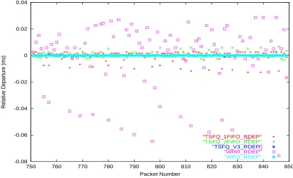
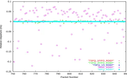
1. Packet departure times: We are interested in showing that TSFQ scheduler versions serve packets in an order similar to that of WFQ, provided that the quantized weights of the flows in TSFQ are the same as the weights of flows in WFQ. Hence, we measure the packet departure order of various versions of TSFQ and WRR relative to WFQ. To compute the departure order of the schedulers relative to WFQ, individual departure times of 100 packets were noted for each schedulerschand then the relative departure of the schedulerrdep_sch was calculated using the formula

rdep_sch=dep_sch−dep_{W F Q} (6.1) wheredep_schand dep_{W F Q}denote the individual departure times of packets under the schedulers sch andW F Q respectively.

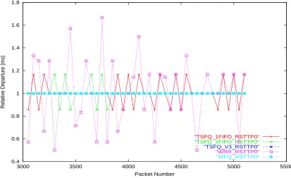
provides better fairness among flows than WRR, we measured the short-term through-put of the packet scheduler. The short-term throughthrough-put of a flow was comthrough-puted by measuring the amount of its bytes served by the scheduler over an interval of 50ms. The relative short-term throughput of the flow served by a schedulersch(RST T P_sch) is then computed using the formula

RST T P_sch= ST T Psch

ST T P_{W F Q} (6.2)

whereST T P_sch andST T P_{W F Q} denote the short-term throughputs of the flow under the schdulers schand W F Q respectively.

3. Average and worst-case delay: Since delay is an important performance measurement for any QoS-aware network, we measured the average and worst-case delay of the flows served by the schedulers.

The following subsections describe each experimental scenario and discusses the results in detail.

6.1

Fixed-Size Packets with a Single Service level

In this experiment, we consider fixed-size packet traffic, and we assume that all flows are assigned to the same service level with weight φ. We simulated 10 flows, which were classified as follows:

• five flows are CBR flows with average rates of 220 Kbps, 350 Kbps, 240 Kbps, 280 Kbps and 160 Kbps.

• three flows are exponential flows with average rates of 190 Kbps, 200 Kbps and 130 Kbps and on/off times of 0.7/0.3, 0.25/0.75 and 0.5/0.5.

• two flows are pareto flows with average rates of 400 Kbps and 200 Kbps and on/off times of 0.5/0.5 and 0.7/0.3.

All the flows generate packets of size 210 bytes and have same weights in all the scheduling techniques.

-0.08 -0.06 -0.04 -0.02 0 0.02 0.04

750 760 770 780 790 800 810 820 830 840 850

Relative Departure (ms)

Packet Number

"TSFQ_1FIFO_RDEP"

"TSFQ_2FIFO_RDEP"

"TSFQ_V3_RDEP" "WRR_RDEP"

"WFQ_RDEP"

Figure 6.2: Relative Departure - Single service level, Fixed-size packets - over all flows

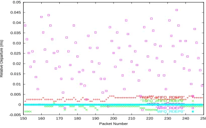
relative to WFQ, the relative departure value of WFQ is always zero. From these figures, we can see that TSFQ V.3 has the same departure order as that of WFQ. These figures also show that the TSFQ versions 1 and 2 differ from WFQ by only a small amount compared to WRR.

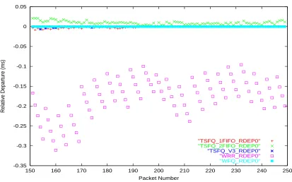
-0.005 0 0.005 0.01 0.015 0.02 0.025 0.03 0.035 0.04 0.045 0.05

150 160 170 180 190 200 210 220 230 240 250

Relative Departure (ms)

Packet Number

"TSFQ_1FIFO_RDEP0"

"TSFQ_2FIFO_RDEP0"

"TSFQ_V3_RDEP0" "WRR_RDEP0"

"WFQ_RDEP0"

Figure 6.3: Relative Departure - Single service level, Fixed-size packets - over Flow 1

6.2

Fixed-Size Packets with Multiple Service Levels

We conducted two sets of experiments for this scenerio, one with a small set of flows and one with a larger set of flows.

6.2.1 Small Set of Flows

In this experiment, we consider fixed-size packet traffic of 20 flows mapped to 5 different service levels with weights 0.05, 0.1, 0.15, 0.25 and 0.4. Each service level has different number of flows mapped to it, with 8 flows getting mapped to service level with weight 0.05, 7 flows mapping to service level with weight 0.15, 4 flows mapping to service level with weight 0.25 and the remaining one flow getting mapped to service level with weight 0.4. The flows generate packets of size 210 bytes and they can be classified as follows:

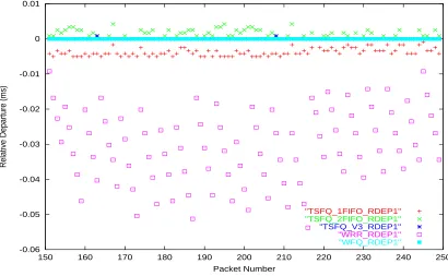
-0.06 -0.05 -0.04 -0.03 -0.02 -0.01 0 0.01

150 160 170 180 190 200 210 220 230 240 250

Relative Departure (ms)

Packet Number

"TSFQ_1FIFO_RDEP1"

"TSFQ_2FIFO_RDEP1"

"TSFQ_V3_RDEP1" "WRR_RDEP1"

"WFQ_RDEP1"

Figure 6.4: Relative Departure - Single service level, Fixed-size packets - over Flow 2

• seven flows are exponential flows with average rates of 90 Kbps, 100 Kbps, 50 Kbps, 80 Kbps, 200 Kbps, 110 Kbps and 130 Kbps and on/off times of 0.7/0.3, 0.5/0.5, 0.8/0.2, 0.7/0.3, 0.2/0.8, 0.5/0.5 and 0.25/0.75.

• three flows are pareto flows with average rate of 150 Kbps and 200 Kbps and on/off times of 0.4/0.6 and 0.5/0.5.