TWO-DIMENSIONAL ELASTO-PLASTIC CRACKED FINITE ELEMENT
FOR DAMAGE DIAGNOSIS
Aysha Kalanad 1, B N Rao 1
Department of Civil Engineering, Indian Institute of Technology Madras, Chennai 600 036, INDIA E-mail of corresponding author: bnrao@iitm.ac.in
ABSTRACT
In this paper a crack identification method based on an improved two-dimensional (2-D) finite element (FE) with an embedded edge crack, and micro genetic algorithm (µ-GA) is proposed. A two-dimensional finite element with a single, non-propagating, open embedded edge crack is developed based on elasto-plastic fracture mechanics. The influence of crack on the local flexibility of the structure is accounted for by the reduction of the element stiffness as a function of the crack length, instead of physically modeling the crack within the element. The proposed element accounts for the influence of crack tip plasticity at the cracked cross-section. The components of the stiffness matrix for the proposed cracked element are derived based on the Castigliano’s first principle. The FRANC2DL finite element code is used with the J-integral option to extract the stress intensity factors from stress
strain fields around the crack tip location, for all the nodal forces. The element is implemented as a user element (UEL) subroutine in the commercial finite element package ABAQUS. The identification of the crack location and depth is formulated as an optimization problem, and µ-GA is used to find the optimal location and depth by minimizing the cost function based on the difference of measured and calculated natural frequencies. The proposed crack detection procedure using the improved two-dimensional finite element and µ-GA is validated using the available experimental and finite element modal analysis data reported in the existing literature.
INTRODUCTION
The presence of a crack in a structural member reduces the stiffness and increases the damping of the structure. As a consequence, there is a decrease in natural frequencies and modification of the modes of vibration. Several approaches have been used to model the problem of a cracked beam using the finite element method. One-dimensional cracked beam finite elements for vibration studies have been developed previously by other researchers [1, 2]. With an aim to simulate the crack presence without actually modeling the crack, more recently a two-dimensional cracked finite element was developed by Potirniche et al. [3] for fatigue and fracture applications.
However, the accuracy of the predicted natural frequency using the cracked finite element developed by Potirniche
et al. [3] for higher values of crack depth ratios is less.
In all the papers cited above, it was assumed that the material around the crack tip behaved in a purely elastic manner. In practice, in many materials, the plastic zone appears around the crack tip, and flexibility of the structure increases more than it is observed for a purely elastic material. Krawczuk et al. [4, 5] developed cracked
beam and plate finite elements, taking into account the effect of plasticity ahead of the crack tip. These efforts used Castigliano’s second theorem, which states that the displacements can be obtained by taking the partial derivatives of the strain energy with respect to the correspondingly applied forces. In a standard finite element implementation, the use of Castigliano’s second theorem is not practical because the resulting singular compliance matrix must be inverted in order to obtain the element stiffness matrix.
This paper presents a crack diagnosis method based on an improved 2-D FE with an embedded edge crack, and µ-GA. A novel two-dimensional finite element with a single, non-propagating, open embedded edge crack, which takes into account the influence of the plastic zone ahead of the crack tip on flexibility of the element is developed. The element is implemented in the commercial finite element code ABAQUS as user element (UEL) subroutine. The identification of the crack location and depth is formulated as an optimization problem, and µ-GA is used to find the optimal location and depth by minimizing the cost function based on the difference of measured and calculated natural frequencies.
ELASTO−PLASTIC CRACKED FINITE ELEMENT
Definition of cracked finite element
{ } {
= 1 2 … 8}
and{ } {
= 1 2 … 8}
T T
F F F F u u u u , (1)
The stiffness matrix of the uncracked element is denoted as ⎡ ⎤0
⎣ ⎦S . In the case of a cracked element, assuming that a crack of length α is present as illustrated in Fig. 1, the stiffness matrix is denoted as
[ ]
S = ⎡ α ⎤⎣S( )
⎦. The force– displacement equation for an uncracked element is then{ }
0 ⎡ ⎤0{ }
= ⎣ ⎦
F S u , (2)
Fig.1: Details of two-dimensional cracked finite element
Due to the crack of length α present at the top edge of the element, and the action of the nodal forces, mode I and II SIFs can be defined as
2 3 1 4
= + = +
I IF IF IF IF
K K K K K , (3)
for mode I due to the nodal tensile forces, and
6 7 5 8
= + = +
II IIF IIF IIF IIF
K K K K K , (4)
for mode II due to the action of the nodal shear forces.
The tensile force at node 3 gives a force and a moment, both of which contribute to an opening of the crack. Hence the contribution KIF3of the nodal force F3 at node 3 is summation of the SIFs given by the force and the
resulting bending moment F h3 2 (h is the element depth), which can be written as
3 = 3+ 3
f m
IF IF IF
K K K , (5)
where
3 3 and 3 3 3
f m
IF f IF m
K =G παF ht K =G πα F ht, (6)
(
)
3 3 3
IF f m
K = G + G παF ht, (7)
with Gf and Gm being the geometrical factors, and t being the element thickness.
It was proposed by Irwin [6] to model the effect of flexibility increasing due to the crack tip yielding by a hypothetical extension of the crack tip rp. The radius of the plastic zone around the crack tip rp, for mode I fracture
of the crack evaluation (opening mode) can be calculated from the following relationship:
(
3)
2 p 2p IF Y
d = r = K σ π, (8)
where σY the material yield strength, and dp denotes the diameter of the plastic zone around the crack tip. It was
also assumed by Irwin that for a crack with the plastic zone around its tip the SIF can be expressed as follows:
(
)
3p 3 3
IF f m eff
K = G + G πα F ht, (9)
where
α = α +eff rp, (10)
with 2
(
)
2p 0.5( f 3 m) Y
r = G + G α σ σ . As can be observed from Eq. (9), an iterative solution technique is usually
required to solve for the SIF. In the first-order estimate, the geometrical factors are computed in the absence of a plasticity correction; then αeff is obtained from Eq. (10), which in turn is used to compute the geometrical factors
f
G and Gm, and subsequently the SIF. Using the SIFs values obtained from FRANC2DL finite element code [7] for
α h ranging from 0.1 to 0.9, and Eq. (6), the geometrical factors Gf and Gm, for the cracked element under tensile
(
)
(
)
(
)
2(
)
3(
)
4(
)
5(
)
62.6233 51.173 551.45 2563.7 5883.6 6472.2 2750.4
f
G αh = − α h + α h − αh + αh − αh + αh , (11)
and,
(
)
(
)
(
)
2(
)
3(
)
4(
)
5(
)
61.6426 18.687 192.08 883.57 2018.3 2213.7 939
m
G αh = − αh + αh − α h + αh − αh + α h . (12)
Contrary to the tensile force acting at node 3 as discussed above, the nodal force F2 acting at node 2 results in a
force that leads to an opening of the crack and a resolved bending moment that leads to the closing of the crack. Hence the contribution KIF2of the nodal force F2 at node 2 can be written as
2= 2− 2
f m
IF IF IF
K K K , (13)
where
2 2 and 2 3 2
f m
IF f IF m
K =G παF ht K =G πα F ht, (14)
(
)
2 3 2
IF f m
K = G − G παF ht, (15)
with the geometrical factors Gf and Gm defined in Eqs. (11) and (12). Similar to that discussed above for the case
of the tensile force acting at node 3, for the case of the nodal force F2 acting at node 2 with a crack having the
plastic zone around its tip the SIF can be expressed as follows:
(
)
2p 3 2
IF f m eff
K = G − G πα F ht, (16)
which allows calculation of the stress intensity factor for an elasto–plastic crack as a function of the area of the plastic zone around the crack tip described by the ratio σ σY, with σ being the applied nominal stress equal to
2
F ht. In Eq. (16), αeff is same as that defined in Eq. (10), with rp=0.5
(
Gf −3Gm)
2α σ σ(
Y)
2. The nodal force F6acting at node 2 gives a shear force and a moment (F w6 ), both of which contribute to mode I and II SIFs, which can
be written as
6 6
2
6 6
6 and
IF I IIF II
K =G πα F w h t K =G παF ht. (17)
Using the SIFs values obtained from FRANC2DL for α h ranging from 0.1 to 0.9, and Eq. (17), the geometrical factors for the cracked element GI and GII respectively, are obtained by curve fitting techniques as a function of
α h as follows,
(
)
(
)
(
)
2(
)
3(
)
4(
)
5(
)
60.821 9.344 96.04 441.78 1009.15 1106.85 469.5
I
G αh = − αh + αh − αh + αh − αh + αh , (18)
and,
(
)
(
)
(
)
2(
)
3(
)
4(
)
5(
)
61.018 17.794 162.7 596.45 1098.3 994.94 353.26
II
G αh = − α h + αh + αh + α h − αh + α h . (19)
Similar to that discussed above for the case of the tensile forces acting at node 2 and 3, for the case of mode I fracture (opening mode) of a crack having the plastic zone around its tip the SIF can be expressed as follows:
6
2 p 6 6
IF I eff
K =G πα F w h t, (20)
with σ being the applied nominal stress equal to 2 6
6F w h t. In Eq. (20), αeff is same as that defined in Eq. (10), with 2
(
)
2p 0.5 I Y
r = Gα σ σ . For mode II fracture (sliding mode) the radius of the plastic zone around the crack tip rp,
can be calculated from the following relationship:
(
6)
2 p 2p 3 IIF Y
d = r = π K σ , (21)
and for a crack with the plastic zone around its tip the SIF can be expressed as follows:
6p 6
IIF II eff
K =G πα F ht. (22)
In Eq. (22), αeff is same as that defined in Eq. (10), with
(
)
2 2
p 1.5 II Y
r = G α σ σ .
Element stiffness matrix derivation
According to the Castigliano’s first theorem the nodal forces Fi can be obtained by taking the partial derivatives of
the elastic strain energy (U) with respect to corresponding displacements (ui)
0 0 and
i i i i
F = ∂U ∂u F =∂U ∂u , (23)
where the index ‘‘0” denotes the undamaged structure. Taking the difference of the above expressions
(
)
0 0
i i i
The difference between the elastic strain energies in the cracked and undamaged cases is related to the SIFs for a fixed displacement case by the relation
(
)
(
)
0 2 2
0
I II
U U t E K K da
α
′
− = − ⌠⎮⌡ + , (25)
where E′ =E for plane stress, E′ =E
(
1− ν2)
for plane strain, E and ν are the modulus of elasticity and Poisson’s ratio. Using Eqs. (24) and (25) for the case of force F3 acting at node 3 and for a crack with the plastic zone aroundits tip
(
)
3(
)
3 30 2
3 3 p 3 p p 3
0 0
2
IF IF IF
F F t E K da u t E K K u da
α α ⎛ ⎞ ⎜ ′ ⎟ ′ − = ∂⎜ ⎟ ∂ = ∂ ∂ ⎝ ⎠ ⌠ ⌠ ⎮ ⎮
⌡ ⌡ . (26)
Substituting Eq. (9) into the above equation and after some simplifications, one obtains,
(
) (
)
20 2
3 3 3 3 3
0
2 f 3 m eff
F F E h t G G a da F F u
α
⎡ ⎤
′
− = π ⎢ + ⎥ ∂ ∂
⎣
∫
⎦ , (27)for a given area of the plastic zone around the crack tip described by the ratio σ σY. In Eq. (27), aeff is same as that
defined in Eq. (10), with
(
)
2(
)
2 p 0.5 f 3 m Yr = G + G a σ σ . In the above equation, the nodal forces for the undamaged and cracked elements can be separated in the two sides of the previous equation and noting from Eq. (2)that
3 3 33
F u S
∂ ∂ = , (28)
the relation between the two forces becomes
(
)
0
3 = +1 33 33 3
F A S F , (29)
where A33 is a constant defined as
(
2) (
)
233
0
2 f 3 m eff
A E h t G G a da
α
⎡ ⎤
′
= π ⎢ + ⎥
⎣
∫
⎦. (30)In Eq. (30), aeff is same as that defined in Eq. (10), with
(
)
(
)
2 2 p 0.5 f 3 m Y
r = G + G a σ σ . Using Eq. (2), Eq. (29)can be written as
(
)
8 8 0
3 33 33 3 1 1
1
= =
= +
∑
j j∑
j jj j
S u A S S u , (31)
which is valid only if the coefficients multiplying the independent variables uj on both sides of the above equation
are equal
(
)
0
3j = +1 33 33 3j
S A S S , (32)
Solving Eq. (32)for S3j the solution is found to be
(
0)
33 1 1 4 33 33 2 33
S = − + + A S A , (33)
and
(
)
0 0
3j 2 3j 1 1 4 33 33 for 1,2, ,8 and 3
S = S + + A S j= … j≠ . (34)
Similarly, for the S2j components, the same procedure indicated above for S3j can be applied
(
)
2(
)
(
)
2
0 2 2
2 2 p 2 22 2
0 0
2 3
IF f m eff
F F t E K da u E h t S G G a da F
α α ⎛ ⎞ ⎡ ⎤ ⎜ ′ ⎟ ′ − = ∂⎜ ⎟ ∂ = π ⎢ − ⎥ ⎣ ⎦ ⎝ ⎠ ⌠ ⎮
⌡
∫
. (35)Thus,
(
)
(
)
20 2
2 22 2
0
1 2 f 3 m eff
F E h t S G G a da F
α
⎛ ⎡ ⎤⎞
′
=⎜⎜ + π ⎢ − ⎥⎟⎟
⎣ ⎦
⎝
∫
⎠ , (36)and the stiffness coefficients are obtained as
(
0)
22 1 1 4 22 22 2 22
S = − + + A S A , (37)
and
(
)
0 0
2 2 2 1 1 4 22 22 for 1,3, ,8 and 2
where A22 is defined as
(
2) (
)
222
0
2 f 3 m eff
A E h t G G a da
α
⎡ ⎤
′
= π ⎢ − ⎥
⎣
∫
⎦. (39)In Eqs. (35), (36) and (39), aeff is same as that defined in Eq. (10), with
(
)
(
)
2 2 p 0.5 f 3 m Y
r = G − G a σ σ . For the case of nodal force F6 acting at node 2, the stiffness components S6j can be obtained adopting the following procedure.
Using Castigliano’s first theorem, the difference between the nodal forces in the cracked (Fi) and undamaged (
0
i
F ) cases can be obtained by taking the partial derivatives of the SIFs with respect to the corresponding displacements (ui) by the relation,
6 6 6 6
0
6 6 p p 6 p p 6
0 0
2 IF IF IIF IIF
F F t E K K u da K K u da
α α ⎡ ⎤ ′⎢ ⎥ − = ∂ ∂ + ∂ ∂ ⎢ ⎥ ⎣ ⎦ ⌠ ⌠ ⎮ ⎮
⌡ ⌡ . (40)
Substituting Eqs. (20) and (22) into the above equation and after some simplifications, one obtains,
(
)
0 2 2 2 2 2
6 6 6 6 6
0 0
2 36 I eff II eff
F F E h t w h G a da G a da F F u
α α
⎡ ⎤
′
− = π ⎢ + ⎥ ∂ ∂
⎣
∫
∫
⎦ . (41)Defining A66 as,
(
2)
2 2 2 266
0 0
2 36 I eff II eff
A E h t w h G a da G a da
α α
⎡ ⎤
′
= π ⎢ + ⎥
⎣
∫
∫
⎦, (42)and noting that
6 6 66
F u S
∂ ∂ = , (43)
the relation between the two nodal forces for the undamaged and cracked elements becomes
(
)
0
6 = +1 66 66 6
F A S F . (44)
In Eqs. (41) and (42), aeff in the first and second terms (inside the brackets) is same as that defined in Eq. (10), with
(
)
22
p 1 0.5 I Y
r = + G a σ σ and rp=1.5G aII2
(
σ σY)
2 respectively. Using{ }
F0 = ⎣ ⎦⎡ ⎤S0{ }
u , Eq. (44) can be written as(
)
8 8 0
6 66 66 6 1 1
1
= =
= +
∑
j j∑
j jj j
S u A S S u , (45)
which is valid only if the coefficients multiplying the independent variables uj on both sides of the above equation
are equal,
(
)
0
6j= +1 66 66 6j for =1,2, ,8…
S A S S j . (46)
Solving Eq. (46) for S6j the solution is found to be
(
0)
66 1 1 4 66 66 2 66
S = − + + A S A , (47)
and
(
)
0 0
6j 2 6j 1 1 4 66 66 for 1,2, ,8 and 6
S = S + + A S j= … j≠ . (48)
Similar formulas can be obtained for all the components S5j, S7j and S8j.
CRACK IDENTIFICATION TECHNIQUE
Selection of variables and objective/fitness function
The µ-GA begins by defining a chromosome, i.e. an array of variables whose values are to be optimized. In our case study the chromosome has two variables, the crack depth ratio (α H) (the ratio of the crack depth (α) to the beam height (H)) and crack location ratio (c L) (the ratio of the crack location (c) to the beam length (L)). Thus we have:
[
]
Chromosome Cracked element number, Crack depth ratio= . (49)
into the mesh at the location defined by cracked element number. Based on the computed natural frequencies from modal analysis using ABAQUS, the objective/fitness function to be minimized is defined as follows:
(
)
*1 Cracked element number,
=
α =
∑
n ω ω − ω ωc i c ii
F H , (50)
where n is the number of frequency ratios being considered, ω ωc i are the natural frequency ratios, which are
functions of the cracked element number and crack depth ratio (α H), and are calculated using the improved 2-D FE, and ω ω*
c i are the natural frequency ratios determined through modal analysis experiments, which are applied to
the crack detection system as inputs (see Fig. 2).
Fig.2: Flowchart of Micro-GA based crack detection method
Chromosome size and encoding
Instead of the standard uniform discretization of the possible interval of the cracked element number and crack depth ratio (α H), they will be assumed to take one value among a discrete set of values in the possible interval. This is done in order to reduce the search space and also to bias the search away from regions of the search space where they assume unrealistic values.
Crack location and crack depth parameters can be an integer in the range 1 2− n and 1 2− m respectively,
with n and m being the number of bits used to encode each possible value of the cracked element number and crack depth ratio (α H). Crack location and crack depth parameters correspond to an entry in the tables of possible values for the cracked element number and crack depth ratio (α H). The tables are built preserving an ordering of increasing crack location ratio (c L) and crack depth ratio (α H), e.g. integer 1 represents less crack location ratio/crack depth ratio than integer 2 and so on. The tables are built according to a recurrent formula. In this way, one fixes the crack location ratio (c L) and crack depth ratio (α H) for the first integer and the next values are increased as follows:
( )
=(
− + ∆1)
, =2, ,2… mc c c
i i i
L L L , (51)
( )
(
1)
, 2, ,2α α α
= − + ∆ = … n
i i i
where ∆c L and ∆α H are the increment of crack location ratio (c L) and crack depth ratio (α H) respectively, for each element of the tables. The values of ∆c L and ∆α H are by the user according to the characteristics of the problem at hand, the available prior information (such as the maximum expected level of the crack location ratio (c L) and crack depth ratio (α H)), and the values n and m adopted. If the exact value of the real crack location ratio (c L) and crack depth ratio (α H) occurring in the structure is not represented in the tables, the c L and α H should go to the closest value of the respective tables. During the search if the crack location and crack depth parameter values falls out of the respective possible entry values in the tables, theirvalues needs to be adjusted or reassigned to an entry in the tables corresponding to INT(possible range × a uniform random number generated between 0 and 1). An individual chromosome is thus a vector of integers (binary encoded) representing a candidate solution that corresponds to a cracked element number and crack depth ratio (α H).
Initial population
In order to determine the appropriate population size in this study, the various population sizes of 5, 8, 10, 12 and 15 individuals, each represented by a vector generated at random, are tested, in numerical Example 1 presented in the subsequent section. The experience gained in the convergence study of Example 1 is used to analyze the problems presented in other numerical examples.
Objective/fitness function evaluation
Natural frequencies are obtained through ABAQUS modal analysis in conjunction with the improved 2-D FE, and the objective/fitness function is evaluated for each chromosome, decoded values of which represent the cracked element number and crack depth ratio (α H).
Convergence criterion
Overall convergence criterion is checked. If the criterion is satisfied, the whole iteration process is stopped; otherwise, continue to the next step. In this study the total prescribed number of generations (= 200) is the overall convergence criterion, and the global algorithm stops when the prescribed number of generations is reached (outer loop).
Reproduction and iterating the algorithm
The population for the next generation is obtained through tournament selection and uniform crossover with a crossover rate of 1.0. The elitism strategy is applied to preserve the best members. Inner loop nominal convergence is checked. If the inner loop does not converge, repeat steps (iv) to (vi). Otherwise, restart and regenerate (replacing the discarded chromosomes in the population by new chromosomes) a new population randomly while keeping the best individual from the previous generation. This replacement of the entire population is for searching the overall space for better solutions in µ-GA. Repeat steps (iv) to (vi).
NUMERICAL EXAMPLE
Patil and Maiti [8] reported natural frequencies obtained by FE analysis of uniform beams with two cracks on three pin supports, starting from one of the simply supported ends. The crack depth was varied from 0.1H to
0.5H (the depth of the beam, H=0.02m). Uniform beam on three pin supports model was made of cross−sectional area 0.02m×0.012m with a length of each span 0.3m. It had the following material properties: Young’s modulus
9 2 210 10
= ×
E N m , density ρ =7860kg m3, the Poisson ratio ν =0.3.
Each span of the uniform beam is modeled with 59 standard four node elements ABAQUS elements and one UEL at the top of the beam. Typical discretization of uniform beam is shown in Fig. 3. For the discretization shown in Fig. 3, the possible values of the cracked element number are 60 i.e. considering one crack in each span the possible value of the cracked element number for the first and second crack is between 61−90 and 91−120 respectively. For the crack depth ratio (α H), 25 possible values in the interval 0< α H<0.5 with an increment of
0.5/ 32
∆α H= are considered. So the cracked element number requires 5 bits, and the crack depth ratio (α H) requires 5 bits, and thus every individual chromosome for uniform beam with two normal edge cracks contains 2×10 = 20 bits.
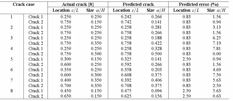
The method for crack identification is verified for several combinations of crack locations and crack sizes listed in Table. 1. The predicted crack locations and crack sizes are in good agreement with the actual values with the average error in the crack location and crack size predictions equal to 1.15 and 3.59 respectively.
Table 1: Comparison of predicted crack positions and sizes of uniform beam with corresponding actual values
CONCLUSIONS
A novel two-dimensional finite element with a single, non-propagating, open embedded edge crack is developed on based on elasto-plastic fracture mechanics. The FRANC2DL FE code is used with the J-integral
option to extract the stress intensity factors from stress strain fields around the crack tip location. The geometric factors for various loading cases of the cracked element for crack depth ratios ranging up to 0.9 are obtained by means of curve fitting techniques, and they are subsequently used to obtain the components of the stiffness matrix for the cracked element from the Castigliano’s first theorem using fracture mechanics concepts. The element is implemented in the commercial FE code ABAQUS as user element subroutine. µ−GA based crack identification methodology to detect crack location and size in conjunction with the improved cracked element is also presented for singularity problems like a cracked beam. The proposed µ−GA based crack detection procedure using the improved 2-D FE is validated using the available experimental and FE modal analysis data reported in the existing literature. The predicted crack locations and crack sizes are in good agreement with the actual values.
REFERENCES
[1] Krawczuk, M., Palacz, M., and Ostachowicz, W., “The dynamic analysis of a cracked Timoshenko beam by the spectral element method,” Journal of Sound and Vibration, Vol. 264, pp. 1139–1153, 2003.
[2] Chondros, T.G., Dimarogonas, A.D., and Yao, J., “Vibration of a beam with a breathing crack,” Journal of
Sound and Vibration, Vol. 239, pp. 57–67, 2001.
[2] Potirniche, G.P., Hearndon, J., Daniewicz, S.R., Parker, D., Cuevas, P., Wang, P.T., and Horstemeyer, M.F., “A two−dimensional damaged finite element for fracture applications,” Engineering Fracture
Mechanics, Vol. 75, pp. 3895–3908, 2008.
[3] Krawczuk, M., Żak, A., and and Ostachowicz, W., “Elastic beam finite element with a transverse elasto−plastic crack,” Finite Elements in Analysis and Design, Vol. 34, pp. 61–73, 2000.
[4] Krawczuk, M., Żak, A., and and Ostachowicz, W., “Finite element model of plate with elasto−plastic through crack,” Computers & Structures, Vol. 79, pp. 519–532, 2001.
[5] Irwin, G.R, “Plastic zone near a crack and fracture toughness,” Proceedings of Seventh Material Research
Conference, Syracuse University, Syracuse NY, pp. 63–78, 1960.
[7] Wawrzynek, P.A., and Ingraffea, A.R., “FRANC2D: Two−dimensional crack propagation simulator, Version 2.7 User's Guide,” NASA CR 4572, 1994.
[8] Patil, D.P., and Maiti, S.K., “Detection of multiple cracks using frequency measurements,” Engineering