NEGATIVE ASSORTATIVE MATING: EXACT SOLUTION TO A SIMPLE MODEL

NEGATIVE ASSORTATIVE MATING: EXACT SOLUTION TO A SIMPLE MODEL*

CATHERINE T. FALKf AND C. C. LI

Department of Biostatistics, University of Pittsburgh, Pittsburgh, Pennsylvania 15213

Received September 16, 1968

HEORETICAL models of negative assortative mating have been studied by

T

F

( 1952)

~

,

WATTERSON

~

~

( 1 959), NAYLOR

~

~

(1 962), WORKMAN (1 964)

,

KARLIN

and FELDMAN (1968)

,

and CANNINGS (1968). F'INNEY discusses certain aspects of two models to which he gives the names zygote and pollen elimination models. WATTERSON and WORKMAN expand upon the tlieoretical implications of the pollen elimination model. KARLIN and FELDMAN discuss some aspects of

FINNEY'S

pollen and zygote elimination models and slight modifications of them. CANNINGS, whose paper treats models with fertility differences between homo- gamous and heterogamous matings, studies the zygote elimination model as a special case of his more general system. In all of these discussions natural selection is assumed to be absent.

In general, systems of recurrence equations employed to describe genetic popu- lations are complicated non-linear, coupled equations. Hence, solutions to such equations of the form p. = f ( p o , n ) , (where p is the frequency of a gene or geno- type and n refers to the generation time)

,

are seldom obtainable. Thus, much of the analysis of such systems has been made by obtaining equilibrium values for the model in question and studying the stability of these equilibria, either locally (see WORKMAN 1964) or, more recently, in the large, defining the domains of attraction for equilibria (KARLIN and

FELDMAN

1968). CANNINGS, in his treat- ment of the zygote elimination model, uses a modified set of non-normalized equations which become linear in form and lead to a single, second-order differ- ence equation. He is able to obtain a solution to the second order equation and then, by renormalizing the frequencies, can study the equilibrium behavior of the system and calculate the heterozygote frequency for any value of n.

In the present paper, FINNEY'S zygote elimination model is discussed further and, using an approach different from CANNINGS', a solution to the equations is presented. In addition, natural selection is introduced into the population and the resulting changes indicated. In order to avoid extra complications in the models, it will be assumed that the population is indefinitely large so that designated matings can take place at appreciable frequencies.

N E G A T I V E ASSORTATIVE M A T I N G WITHOUT SELECTION

Consider a population in which two alleles, A and a, are segregating at an auto- * Supported by grants 2 TO1 GM 00039 and HE 09011 from The National Institutes of Health, Bethesda, Maryland.

t Presest address: Department of Serology and Genetics, The New York Blood Center, New York, New York 10021.

216 C . T. FALK A N D C . C . LI

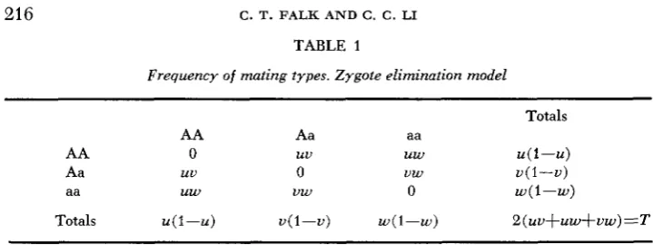
TABLE 1

Frequency of mating types. Zygote elimination model

~ ~ ~

Totals

AA Aa aa

AA 0 uu uw u ( 1 - U )

Aa uu 0 uw u ( 1 - U )

aa uw uw 0 w(1-w)

Totals u(1-U) u ( 1 - U ) w(1-w) &(uu+uw+vw)=T

soma1 locus. Let the frequencies of genotypes AA, Aa, aiid aa in the population be U , U and w, respectively; L E + u + w = ~ . As in FINNEY’S zygote elimination model, let the frequency of matings between like phenotypes be zero, and between all others be those expected in a random mating population. Assume that no selection is acting upon the characteristic being considered. If the A allele is dominant, so that genotypes AA and Aa are indistinguishable, there will be only one type of mating possible, namely A- with aa. From such matings no AA offspring are possible and after two generations of mating the ratio of Aa individuals to aa’s will be 1:l (LI, 1955, p. 234).

If there is no dominance, the frequencies of the various mating possibilities in a particular generation will be as given in Table 1 . Tlie frequencies of the three genotypes in the offspring generation will be

u n + 1 = unun/Tn ( 1 )

un+1= ( ~ , ~ n + 2 ~ n ~ n + ~ ’ n w n ) / T n

,

( 2 )

wn + 1 unwn/Tn ( 3 ) where the subscript n denotes the generation and

thus normalizing the three frequencies at each generation. This set of equations describes FINNEY’S zygote elimination model. As he points out, if all of the fre- quencies are non-zero,

Tn = 2 (Un~n+~nmn+~nWn)

( 4 )

um+~ - un

-

W n + 1 W n

= K>O

.

That is, the ratio of the homozygote frequencies in any generation is a constant. Using this relationship between U and w, equilibrium values for the genotypes can he obtained. These are:

ue = Kwe

,

( K - 1 ) 2,+ ( 1 + K ) V‘ ( 1 + K ) ‘ f 8 K

4( 1 + K f K 2 ) ~e = l-We(l+K) =

and

2

3 ( 1 + K ) +d/(lfK)”+8K ‘

we = ₍₇₎

These correspond to the entries for Model 1’ in Table 5 cf KARLIN and FELDMAN ( 1 9 6 8 ) .

NEGATIVE ASSORTATIVE M A TI N G

Figure 1.

21 7

locus of equilibria

V

V V

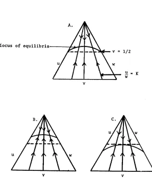
FIGURE 1 .---Complete Negative Assortative Mating without Dominance.

U

W - = K

A. No selection, - 1

<

ue

<

vz

2 3

8 2

B. a = b = 2, h = 8,-

<

ue

<

-

13 3

2 1

C. a = b = 2 , h = 1,-

<

U,

<

-

5 2

218 C . T. FALK A N D C. C. LI

where pe and qe are the equilibrium frequencies of A and a in the population, or equivalently

Because of the restriction p+q=l, upper and lower bounds may be obtained for ue. These are:

~ , ( ~ . , - 0 . 5 ) = u e w e .

-

0.5

<

U , 5 ''

5

=

0.57735 .

3

If an endpoint solution is allowed so that either u=O or w=O, then ~ e r O . 5 . Such an equilibrium is reached in one generation of mating.

In order to specify completely the "movement" of the population from genera- tion to generation, solutions of the form w,=f(w,,K,n) can be obtained for equa- tions ( l ) , (2 ) and (3). Equations ( 2 ) and (3) can be rewritten

W n = [I (K+l)un+2Kw,]

--

Tn

and

Consider the ratio

u n + 1 - (K+l)vn+2Kwn --

W n + 1 u n

Let V , be the vector

(

w,

"9

and

Q

the matrix

(

K+l 1

2K>

0

.

The matrix difference equation

V n

+

1 = QVn ( 8 )

can then be used to obtain the ratio vn/wn. The solution to (8) is V,=Q"V,. The matrix

Q

iiiay be diagonalized by standard techniques. Let h1 and X 2 be the posi- tive and negative eigenvalues of Q, respectively, and le t

P

be a matrix such that

The eigenvalues of Q are the roots of the quadratic equation: Theref ore,

A'- ( 1 + K ) h-2K=0.

l + K + q ( 1 f K ) *+8K

2

A =

Let 1, be the positive root and A, the negative root. Then In terms of hl, h2 and the original genotype frequencies,

V , = (IrlQdnP) V ,

.

)

1

V , = -

Thus the ratio,

U,- _uo(Xz,+l-h 1 ,+l

1

f W O h l X 2 (X1"-X2">

w, U o ( h p , - h l n ) 3- W,h,Xz (hln-l-hZ~--l) *

NEGATIVE ASSORTATIVE MATING 21

9

Let

(2)

= E where / E /

<

1. Then

(10) - uo ( EnAz-&i) fWoXiXz ( l - E n )

--

W n Do ( E n - 1 ) + W O (Az-AiEn)

For n very large E , approaches zero, so, in the limit, as n + 00, ue

-

-uoXi+woXihz

-

W e

-UofWoXz

- X i

.

--

This is in agreement with the equilibrium values obtained in equations (6) and (7), as (6)/(7) = XI, on simplification.

Substituting u,=l-w, (1 f K ) into equation (10)

E"(uo-hiWo) f (Xzwo-uo)

~ ~ ( X z f l f K ) ( ~ ~ - - h ~ ~ o ) f ( X ~ + l f K ) ( X Z W O - D O ) ' W n =

1

But, by ( 7 ) -= 1 S K f X i We

and

X2wo-uo=wo(

1 f K f h z ) - l .

WO 1

where p=l-- and y=- - (1 4-K) 2+8K

me

We

For example, if uo = .4,

w o

= .2, and thus K=2, the frequency of aa in the popu- lation for various values of n will be

n I 0 1 2 3 4 5

. . . .

n > 8

w n

.2000 .12500 .14706 .14179 .14312 .14279

. .

.

.

.14286

These values of

w,,

obtained from equation ( 11 )

,

are in agreement with the values obtained by repeated iteration of equations (1 )

,

(2), and (3). Because one of the eigenvalues is negative, the approach to equilibrium is oscillatory in nature. A genotype frequency is successively greater than and less thhnn the equilibrium value as it damps out in its approach to equilibrium.

The "stability" of this equilibrium is somewhat different from that generally encountered in genetic models. If a disturbance of the frequencies occurs at any time in such a way as to change the value of K, the system will move towards a new equilibrium dependent upon that new K instead of going back to the old K. This is similar to the Hardy-Weinberg equilibrium for a simple random mating model where the initial gene frequencies determine the equilibrium and a dis- turbance of the gene frequencies changes the equilibrium. For the random mating model, such an equilibrium is reached after one generation of mating. For this assortative mating model, the approach is slower.

N E G A T I V E ASSORTATIVE MATING WITH SELECTION

220 C . T. FALK A N D C . C . LI

Tun+l= a(unvn)

,

(12)

T v n + l = h ( ~ n v n S 2 ~ n ~ n S v n ~ n )

,

( 1 3 )

Twn+,l= b(vnwn)

,

( 1 4 ) where T i s defined so that U n + i f v n + i + w n + l = l .

First, consider a and b not equal, specifically taking a<b. If all frequencies are non-zero, the ratio of equations (12) and (14) will be

Let the vector U, =

(

"

)

.

Wn

Then the ratio U n + l / w n + 1 can be represented by the vector difference equation

The solution, U, =

(%)n

U,, implies that the ratio un/wn approaches zero as n approaches infinity. This implies that un also approaches zero with increasing n.

If U and w both remain non-zero (a necessary condition if the population is to survive)

h

v e = - b+h and

b

We=--

b+h *

For a

>

b the argument can be used on the reciprocal of equation (15) showing that wn approaches zero as n increases. Then,

a

ue = - h+a

h h+a

.

and U, =

-

If neither U nor w is zero at equilibrium then T = av and

T

= bv. Since U can never be zero at equilibrium in a complete negative assortative mating model,

a and b must be equal.

Here, as in the model without selection, the ratio

5

is always a constant. All oi the argunients of the preceding section can again be used to obtain the equilibrium values, again falling along a quadratic curve, an exact solution to the recurrence equations, and upper and lower bounds on the equilibrium values for U . Without repeating the steps, the pertinent results will be included here. Again assuming un, wn f 0 and letting

Wn

u n

Wn

NEGATIVE ASSORTATIVE M A T I N G 221

h(K-l>’+ (1+K) .\/h2(1+K)2+SahK 2[a(l+2q2

+

h(KZ+l)l

ve = 7

and

242

(2a+h) (1

+ K )

f

d h 2

( 1 + K ) *+8ahK

we =

The locus of equilibrium values in terms of

v

is given by ve = 2

dp*

,

and the bounds on ue are

2a+h

For a = h, i.e. no selection, all of these results reduce to those in the previous section.

An exact solution to equations (12), (13), and (14) is found by again using the matrix difference equation technique. The simplilied ratio equation from equations (13) and (14) is

v n + 1

-

h[un(l,+K) +2wnKI

--

W n + 1 aun

h ( l + K ) 2hK

Let Q l = (

_.

b 0

)

bethe

matrix of coefficients, A3 and X4 be the eigenvalues of

Q1,

and

P,

be a matrix such that

P,Q,P,-’=

0 h

’)

=

( Q l ) d .

ha and AB will be the positive and negative roots of

h ( 1

S K )

f L<h2 (1 + K ) 2+8ahK

2

A =

respectively

.

L e t A = E , w h e r e l e , l < l

,

As

a f a K S A 4 = y 1

WO

We a n d l - - = p . Then

(16)

a&lnp+woyl-a

W n =

EInpY1+(l/me.) (woy1-a) *

As before the approach to equilibrium is oscillatory. If a is set equal to h, equation (1 6) reduces to equation ( 1 1 )

.

Figure 1 shows the locus of equilibria and paths of approach for models with selection where the heterozygote is more fit than the homozygotes, (part B) and where the heterozygote is less fit, (part C )

.

DISCUSSION

222 C. T. FALK AND C . C . LI

the maintenance of a balanced polymorphism in a population. Negative assorta- tive mating, by its nature, is a sort of selection favoring heterozygotes. In the zygote elimination model such a mating system, in the absence of other selective forces, is able to maintain a high frequency of heterozygosity in the equilibrium population.

Comparison of this model with a simple random mating model without selec- tion yields some similarities as well as some differences. Each has a locus of equilibria determined by the original conditions. In random mating the condi- tions are the gene frequencies; in assortative mating they are the genotype fre- quencies. In random mating, equilibrium is reached after one generation; in as- sortative mating, only if one homozygote has a zero frequency will equilibrium be reached in one generation. Otherwise the approach is slower and is oscillatory in nature. Each equilibrium curve is a quadratic function. The equilibrium for any given case will be altered if, in the random mating model, the gene frequen- cies are altered, and, in the assortative mating model, if the ratio of homozygote frequencies, is altered. Thus neither equilibrium is “stable” in the usually ac- cepted sense. In random mating the maximum heterozygote frequency attainable is

1/2,

reached when the gene frequencies are equal. In assortative mating the maximum heterozygote frequency is also obtained when the gene frequencies are equal, but it is somewhat greater than

%.

The minimum heterozygote fre- quency is in fact

1/2.

The introduction of selection parameters into the negative assortative mating model alters the picture somewhat.

If

the two homozygotes have unequal selec- tion values the “less fit” homozygote will eventually disappear from the popula- tion and an equilibrium will be maintained between the other homozygote and the heterozygote. If the two homozygotes are equally fit but different from the heterozygote, a situation that may be improbable in nature, the pattern of equi- libria and approaches will be similar to the model without selection. The main difference lies in the upper and lower bounds placed on the equilibrium heterozy- gote frequencies (see Figure 1). If the heterozygote is more fit than the homozy- gotes, the two existing forces, (selection and mating)

,

will be working together to increase the frequency of heterozygotes. Hence the equilibrium curve will be “higher” on the graph, relative to the model without selection. If the heterozy- gote is less fit, this selective force will oppose the mating system’s influence and the equilibrium curve will be lower.

NEGATIVE ASSORTATIVE M A T I N G 223

heterozygote superiority offers a possible explanation for unusually high frequen- cies of heterozygotes in natural populations which are in apparent equilibrium.

by C. CANNINGS (1968).

The authors would like to thank one of the referees for bringing to their attention the article

SUMMARY

A

model of negative assortative mating, with inviability of zygotes from mat- ings between like genotypes, has been investigated and a general solution is pre- sented. The resulting equilibria, paths of approach to equilibria, and conditions necessary for the existence of balanced polymorphisms are set forth for models with and without selection.

LITERATURE CITED

CANNINGS, C., 1968 Fertility differences between homogamous and heterogamous mating. Genet. Res., 11 : 289-301.

FINNEY, D. J., 1952 The equilibrium of a self-incompatible polymorphic species. Genetica

26: 33-64.

KARLIN, S., and M. W. FELDMAN, 1968 Further analysis of negative assortative mating. Genetics

LI, C. C., 1955 NAYMR, A. F., 1962.

WATTERSON, G. A., 1959

WORKMAN, P. L., 1964

59: 117-136.

Popuhtion Genetics. University of Chicago Press.

Mating systems which could increase heterozygosity for a pair of alleles.

Non-random mating, and its effects on the rate of approach to homozy-

The maintenance of heterozygosity by partial negative assortative Am. Naturalist, 96: 51-60.

gosity. Ann. Human Genet. 23 : 204-220.