Article
Assessing Uncertainty in LULC Classification
Accuracy by Using Bootstrap Resampling
Lin-Hsuan Hsiao 1 and Ke-Sheng Cheng 2,3,*
1 Newegg, Inc., Taipei 10596, Taiwan; [email protected]
2 Department of Bioenvironmental Systems Engineering, National Taiwan University, Taipei 10617, Taiwan 3 Master Program in Statistics, National Taiwan University, Taipei 10617, Taiwan
* Correspondence: [email protected]; Tel.: +886-2-3366-3465
Abstract: Supervised land-use/land-cover (LULC) classifications are typically conducted using class assignment rules derived from a set of multiclass training samples. Consequently, classification accuracy varies with the training data set and is thus associated with uncertainty. In this study, we propose a bootstrap resampling and reclassification approach that can be applied for assessing not only the uncertainty in classification results of the bootstrap-training data sets, but also the classification uncertainty of individual pixels in the study area. Two measures of pixel-specific classification uncertainty, namely the maximum class probability and Shannon entropy, were derived from the class probability vector of individual pixels and used for the identification of unclassified pixels. Unclassified pixels that are identified using the traditional chi-square threshold technique represent outliers of individual LULC classes, but they are not necessarily associated with higher classification uncertainty. By contrast, unclassified pixels identified using the equal-likelihood technique are associated with higher classification uncertainty and they mostly occur on or near the borders of different land-cover.
Keywords: land-use/land-cover (LULC); uncertainty; bootstrap resampling; chi-square threshold; class probability vector (CPV); entropy
1. Introduction
significance of differences in classification accuracy [31]. It has been suggested to fit confidence intervals to the estimates of classification accuracies and consider these intervals when evaluating the thematic map [32]. However, the confidence intervals of classification accuracies are often calculated under the assumptions that training data are normally distributed and they represent random samples of individual LULC classes. In reality, training data may be non-Gaussian and data independency is not guaranteed because of the spatial autocorrelation of reflectance of individual land-cover types. For example, ground data collection is frequently constrained because physical access to some sites is impractical; thus, the collection is restricted either to sites of opportunity (where obtaining ground data is possible) or sites for which high-quality fine spatial resolution images acquired at an appropriate date are available as a surrogate for actual ground observations [33]. Such sampling practices further complicate the statistical assessment of LULC classification accuracy. In addition to the training data uncertainty, other factors, such as errors in georeferencing, the existence of mixed pixels, and the selection of probability distribution models, can also affect the LULC classification accuracy.
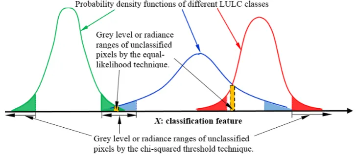
In most applications of LULC classification, each individual pixel is assigned to one of the reference classes. If a pixel falls near the tail of the multivariate distribution established by the training data, it may be desirable to assign that pixel as unclassified. Assuming multivariate Gaussian (normal) distributions for reflectance-vectors of individual LULC classes, class-dependent thresholds for labeling unclassified pixels can be determined on the basis of a chi-square distribution [34]. Unclassified pixels identified using the chi-square threshold technique represent the outliers of individual LULC classes, but they do not necessarily represent pixels with nearly identical likelihoods of belonging to different LULC classes. These situations are illustrated in Figure 1 by using a one-dimensional classification feature. However, in practice, pixels with nearly identical likelihoods of belonging to different LULC classes may need to be designated as unclassified pixels. Hereafter, we refer to such pixels as pixels of equal likelihood. Because the joint probability densities of the classification features of different LULC classes are estimated using the selected training data, the aforementioned training data uncertainty eventually leads to uncertainty in the estimated joint probability densities of the classification features of individual LULC classes and decision rules of the LULC classification. Consequently, the identification of pixels of equal likelihood is further complicated by the uncertainty in the joint probability density estimates of the classification features.
Figure 1. Illustration of the ranges of the classification feature of unclassified pixels identified using the chi-square threshold and equal-likelihood techniques.
bootstrap resampling technique, application of bootstrap resampling to multispectral remote sensing images, and the assessment of LULC classification uncertainty. In Section 4, we present the LULC classification results derived from the original training data and reclassification results derived from the bootstrap-training samples. Detailed discussions on the uncertainty of various classification accuracies and the characteristics of unclassified pixels that are identified using the chi-square threshold technique and equal-likelihood technique are also included in Section 4. A summary of the findings and concluding remarks are presented in Section 5.
2. Study Area and Data
The Greater Taipei area was selected as the study area. It encompasses approximately 360 km2 and has a highly populated urban area, a national park in the northeast corner, and mountains in the southeast corner. The confluence of three major rivers in northern Taiwan is in the northwest corner of the Taipei City. Advanced Land Observing Satellite (ALOS) multispectral images of the study area (acquired on 5 April 2008, by the AVNIR2 sensor) were collected. The AVNIR2 sensor acquires images in four spectral bands, namely blue (0.42–0.50 µm), green (0.52–0.60 µm), red (0.61–0.69 µm), and near infrared (NIR, 0.76–0.89 µm), at a spatial resolution of 10 × 10 m. All of these satellite images are preprocessed for radiometric and geometric corrections by the Japan Aerospace Exploration Agency [35]. Thus, all images were georeferenced to map-projection coordinates. A true-color image of the study area and an official land-use map obtained from the Ministry of Interior of Taiwan [36] are presented in Figure 2.
Figure 2. (a) True-color Advanced Land Observing Satellite (ALOS) image of the study area; and (b) land-use map for the year 2009 (Ministry of Interior, Taiwan). The purple-circled area, the Beitou Depot of the Taipei mass rapid transit (MRT), is identified as unclassified by the chi-square threshold technique (see details in Section 4.2.3). The coordinates of the lower-left corner of panel (a) are 121°25′50″E, 24°59′12″N.
scattering of different LULC classes in a three-dimensional feature space, digital numbers of the green, red, and near infrared (NIR) bands were selected as classification features in this study.
Table 1. Numbers and proportions of training pixels of individual land-use/land-cover (LULC) classes.
LULC Classes Forest Water Buildings Grass Roads Number of training pixels 7005 2771 5956 2445 3924
Proportions (%) 31.70 12.54 26.95 11.06 17.75
Figure 3 is a scatter plot of training pixels of different LULC classes in the three-dimensional green–red–NIR feature space. In the figure, the training pixels of the forest and water land-cover types are more concentrated than the other land-cover types. By contrast, the training pixels of buildings and roads are widely dispersed and mutually mixed.
Figure 3. Scatter plot of the training pixels of LULC classes in the green–red–NIR feature space.
3. Methods
The supervised Bayes classification method was chosen for the LULC classification task in this study. The bootstrap resampling technique was also applied to the original training data set described in Section 2 to generate resampled training data sets that were used in the subsequent Bayes classification task.
3.1. Bayes Classification
In the Bayes classification method, the a priori probabilities of individual land-cover types in the study area are considered. The a priori probability of a particular class represents the probability of a randomly selected pixel belonging to that class. Although not necessary, most LULC applications assume multivariate Gaussian distributions for the classification features of different LULC types. Let X =(x1,,xk)T be a k-dimensional feature vector of a particular pixel and let p(
ω
i) (i=1,,N) be the a priori probabilities of N LULC classes. The joint Gaussiandensity of the ith class
(
ω
i)
is expressed by(
)
1(
)
1 2
1
1
( | )
exp
2
2
π
T
i k i i i
i
f X
ω
=
−
X
−
μ
Σ
−X
−
μ
where
μ
i and Σi are, respectively, the mean vector and covariance matrix of the classification features of the i-th class. The class-dependent discriminant function of the Bayes classification method is defined as follows:(
) (
)
, 1,2, , . 21 ln 2 1 ) ( ln )
(X p X 1 X i N
d T i i
i i
i
i = ω − Σ − −μ Σ− −μ = (2)
A pixel with feature vector X is assigned to the i-th class if di(X) is the highest of all class-dependent discriminant functions; that is,
. every for ), ( )
(X d X j i
di > j ≠ (3)
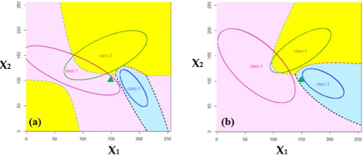
The work of LULC classification by using multispectral remote sensing images can be perceived as the partitioning of a k-dimensional feature space into different regions associated with different LULC classes. Pixels with equal values of discriminant functions form the class boundaries in the feature space. An example of the three-class partitioning of a two-dimensional feature space by using the Bayes classification method is illustrated in Figure 4. The classification features of the individual classes in Figure 4a,b, are assumed to follow bivariate Gaussian distributions with the parameters listed in Table 2.
Figure 4. Exemplary illustration of the three-class partitioning of a two-dimensional feature space derived from the Bayes classification method. The classification features (X1 and X2) of individual classes in Panels (a) and (b) are characterized by multivariate Gaussian distributions with the parameters listed in Table 2. The ellipses represent the 95% probability contours of individual classes, and the dashed lines are the boundaries of different classes. Regions belonging to different classes are shown in different colors. A sample point (marked by ) is classified into different
classes under different distribution parameters.
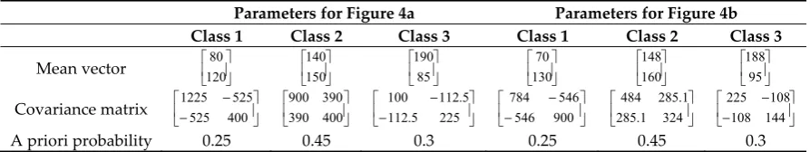
Table 2. Parameters of the bivariate Gaussian distributions of the individual classes in Figure 4.
Parameters for Figure 4a Parameters for Figure 4b Class 1 Class 2 Class 3 Class 1 Class 2 Class 3
Mean vector
120 80 150 140 85 190 130 70 160 148 95 188
Covariance matrix − − 400 525 525 1225 400 390 390 900 − − 225 5 . 112 5 . 112 100 − − 900 546 546 784 324 1 . 285 1 . 285 484 − − 144 108 108 225
A priori probability 0.25 0.45 0.3 0.25 0.45 0.3
3.2. Bootstrap Resampling and Its Application to Multispectral Remote Sensing Images
Bootstrapping, which was first introduced by Efron [37], is a statistical technique of generating random samples and estimating the distribution of an estimator of a population by sampling with replacement from a random sample or a model estimated from a random sample of that population. It amounts to treating the data as if they were the population for the purpose of evaluating the distribution of interest. Bootstrapping provides a means to substitute computation for mathematical analysis when calculating the asymptotic distribution of an estimator or statistic is difficult [38]. Bootstrap resampling has been applied to LULC classification using remote sensing images to improve the characterization of classification errors, determine the uncertainty resulting from sample site variability, and calculate the confidence limits of classification errors [39].
Let
X
1,
,
X
n be a random sample of size n from a probability distribution whose cumulative distribution function (CDF) isF0. The empirical CDF ofX
1,
,
X
n is denoted asF
n. LetF
0 belong to a finite- or infinite-dimensional family of distribution functions, F. If F is a finite-dimensional family indexed by the parameterθ
, whose population value isθ
0, we write) ,
( 0
0 x
θ
F for P(X ≤x) and F(x,θ) for a general member of the parametric family. Let
)
,
,
(
1 n nt
X
X
T
=
be a statistic andG
n(
τ
,
F
0)
≡
P
(
T
n≤
τ
)
denote the exact, finite-sample CDF ofT
n. In addition, letG
n(
⋅
,
F
)
denote the exact CDF ofT
n when the data are sampled from thedistribution whose CDF is
F
. The bootstrap estimator of Gn(⋅,F0) isG
n(
⋅
,
F
n)
which can beestimated through the following Monte Carlo simulation procedure, in which random samples are drawn from X1,,Xn [38]:
1. Generate a bootstrap sample of size n, X1*,,Xn* by sampling with replacement from the
random sample X1,,Xn. Note that using an asterisk to indicate bootstrap samples is customary.
2. Calculate
T
n*=
t X
(
1*, ,
X
n*)
.3. Repeat Steps 1 and 2 many times and use the resultant Tn*i, i=1,,B to derive the empirical
CDF of Tn*; that is,
) ( ) , (
τ
*τ
≤ = n nn F PT
G . (4)
When the bootstrap resampling technique is applied to remote sensing LULC classification, the training data of a particular LULC class are considered as the original sample
X
1,
,
X
n, and the bootstrap samples (X )j (X*, ,Xn*)j1
* = ( j=1,,B ) are generated by resampling from
n
X
X
1,
,
. This process is detailed as follows.Suppose N land-cover classes (
ω
i, i=1,,N) are present in the study area. Let N i S S i n ii , 1, ,
,
, ()
) (
1 = represent the training pixels of the i-th class, where ni (i=1,,N) is the number of training pixels. Each training pixel, for example,
S
1(i), corresponds to a k-dimensionalfeature vector X1(i) =(X1,,Xk)1(i). The following simulation and calculation steps are performed
1. Obtain the bootstrap training samples S i Sni i N i , 1, ,
,
, *()
) *(
1 = by sampling with replacement from the original training samples of the individual land-cover classes (i.e.,
N i S S i n i
i , 1, ,
,
, ()
) (
1 = ).
2. Collect the corresponding multispectral feature vectors X i X i Xni i N i ), 1, ,
, , ( *() *() 1 ) *( = =
with X1*(i) =(X1,,Xk)1*(i). Note that
X
*(i),
i
=
1
,
,
N
represents feature vectors of one set of multispectral and multiclass bootstrap training samples.3. Repeat Steps 1 and 2 to obtain B sets of multispectral and multiclass feature vectors of bootstrap training samples; that is,
( )
X i j X i Xni j i N j Bi ), 1, , ; 1, ,
, , ( *() *() 1 ) *( = = = .
4. Estimate the parameters of the multivariate Gaussian distribution for every set of multispectral and multiclass feature vectors of the bootstrap training samples. Let estimates of the mean vector and covariance matrix of the multispectral and multiclass feature vectors be represented by
( )
j i) *(
ˆ
μ and
[ ]
Σˆ*(i) j, i=1,,N; j=1,,B, respectively.5. For every set of multispectral and multiclass bootstrap training samples, calculate the class-dependent discriminant functions (Equation (2)) of the individual land-cover classes by using the parameters estimates from Step 4 and perform LULC classification for all pixels in the study area. Note that all bootstrap training samples are associated with known LULC classes and are treated as training data in the bootstrap-sample-based LULC classification. However, in contrast to the original training samples, these bootstrap samples are not associated with specific geographic locations in the study area.
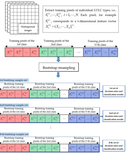
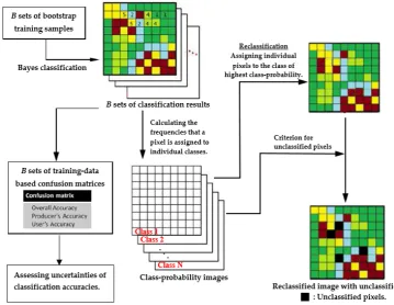
A schematic diagram of the aforementioned bootstrap resampling and classification procedures is depicted in Figure 5. Notably, by using B sets of bootstrap training samples for LULC classification, we can assess not only the uncertainty in the classification of the bootstrap training samples, but also the uncertainty in the class assignment of individual pixels in the study area.
3.3. Assessing Classification Uncertainty by using Bootstrap Samples
The classification accuracy of the training data can be evaluated by using the training-data-based confusion matrix. In a confusion matrix, the class-dependent producer’s accuracy (PA) and user’s accuracy (UA), and the overall accuracy (OA) are presented. However, the training-data-based confusion matrix can assess only the classification accuracy (or errors) of the training data. Furthermore, studies have also evaluated classification accuracy by applying decision rules derived from training data to an independent set of reference data. For such applications, reference-data-based confusion matrices have been established to evaluate the classification accuracy of the reference data. When only one set or a limited number of sets of reference data are used, the reference-data-based confusion matrices are unlikely to represent the classification accuracy of the entire study area. In light of the uncertainties, several questions that require consideration in remote sensing LULC classification are as follows:
What is the probability that a pixel that is randomly and equally likely to be selected from the set of all pixels in the study area is correctly classified? This probability is referred to as the global OA (as opposed to the OA of the training data set).
Let the set of all pixels that are assigned to the i-th class be denoted as S(Ai). What is the probability that a pixel that is randomly and equally likely to be selected from SA(i) is correctly classified? This probability is referred to as the class-specific global UA.
Figure 5. Schematic of bootstrap resampling of the training samples and its application to multispectral and multiclass LULC classification.
Estimating these probabilities is complex when all of the sources of uncertainty addressed in the Introduction require consideration. These probabilities cannot be exactly known, and we can estimate them only according to the classification results derived from the training data set. In this study, we focused on estimating these probabilities by considering only the training data uncertainty. A bootstrap-resampling-based approach is proposed in this study. The details of the approach are as follows:
1. Determine the a priori probabilities of individual LULC classes; that is, p(
ω
i) (i=1,,N).These probabilities are estimated on the basis of ancillary data or the investigator’s knowledge of the study area.
and uncertainty to be representative of the entire study area or be considered estimates of the classification accuracy and uncertainty for the entire study area.
3. Conduct bootstrap resampling to obtain B sets of bootstrap training samples.
4. For each set of the bootstrap training samples, determine the Bayes classification decision rules of the individual LULC classes and conduct LULC classification for the entire study area. Subsequently, establish the corresponding bootstrap-training-sample-based confusion matrices. Because bootstrap samples have different distribution parameter estimates and class-dependent discriminant functions, their confusion matrices vary among different bootstrap samples, enabling the assessment of the uncertainty in the classification accuracy. 5. For any pixel in the study area, calculate the frequency it is assigned to an individual LULC
class. Let b(i) represent the frequency that a particular pixel is assigned to
ω
i (i=1,,N);then, its class probability vector (CPV) is defined as
=
=
B
N
b
B
b
p
p
P
N
(
)
/
/
)
1
(
1
ω ωω . The
pixel-specific CPV represents the probabilities that a pixel will be assigned to individual LULC classes (i.e., pixel-specific class probabilities). These probabilities can then be used to characterize the location-specific classification uncertainty and generate a set of class-probability images.
6. Reclassify the study area by assigning individual pixels to the class of the highest class probability. In this study, this process is referred to as bootstrap-based LULC reclassification. 7. Identify unclassified pixels by using the predetermined threshold p*max (for example,
9 . 0
* max=
p ) for the highest class probability. A pixel with class probabilities
= B N b B b
PωT (1) ( ) is identified as unclassified if *
max max ) ( , , ) 1 ( max p B N b B b
p <
= .
An analytical flowchart of the proposed LULC classification by using bootstrap-based LULC reclassification is depicted in Figure 6.
4. Results and Discussion
4.1. LULC Classification Results Based on the Original Training Data Set
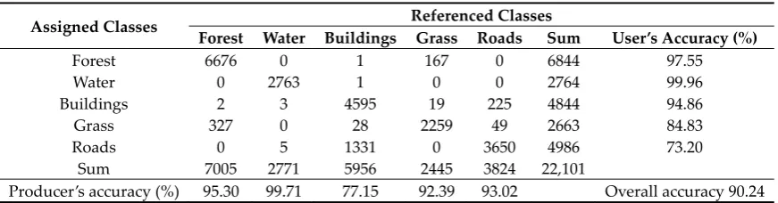
Derived from the original training data set (Table 1), the training-data-based confusion matrix and Bayes LULC classification results of the study area are shown in Table 3 and Figure 7a, respectively. Misclassifications primarily occurred between the forest and grass land-cover classes and between the buildings and roads land-cover classes. In particular, a significant portion (approximately 23%) of the pixels of the buildings class were misclassified into the roads class, whereas only 7.5% of the pixels of the roads class were misclassified into the buildings class.
Figure 7. LULC classification results: (a) based on the original training data set; and (b) based on the bootstrap training data sets and the highest class probability. The purple-circled area is the main structure of the Beitou Depot of the Taipei MRT (see Section 4.2.3). (c,d) Magnified images of the red-square-enclosed areas in Panels (a) and (b), respectively.
Table 3. Confusion matrix of LULC classification by using the original training data set.
Assigned Classes Referenced Classes
Forest Water Buildings Grass Roads Sum User’s Accuracy (%)
Forest 6676 0 1 167 0 6844 97.55
Water 0 2763 1 0 0 2764 99.96
Buildings 2 3 4595 19 225 4844 94.86
Grass 327 0 28 2259 49 2663 84.83
Roads 0 5 1331 0 3650 4986 73.20
Sum 7005 2771 5956 2445 3824 22,101
4.2. Bootstrap-Based LULC Reclassification Results
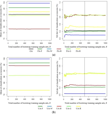
Bootstrap resampling of the original training data set was implemented in this study, yielding B sets of bootstrap training samples. As illustrated in Figure 6, the Bayes LULC classification results vary among the bootstrap training data sets. Because the uncertainty of classification accuracy was evaluated on the basis of B sets of bootstrap-training-data-based confusion matrices, we investigated the effect of the number of bootstrap samples (B) on the uncertainty in the LULC classification accuracy. We repeatedly generated bootstrap training data sets with the total number of bootstrap samples; specifically, B varied from 10 to 1000 in increments of 10. On the basis of B sets of training-data-based confusion matrices, we calculated the mean and standard deviation for each of the UA, PA, and OA. Figure 8 shows that the mean classification accuracy remains nearly constant, regardless of the value of B. By contrast, the standard deviation of the classification accuracy changes with the number of bootstrap samples for 10≤B≤400 but remains approximately constant for B≥500. These results indicate that, based on our original training data set, at least 500 sets of bootstrap training samples must be used when assessing the uncertainty of classification accuracy. Therefore, the subsequent analysis of the classification accuracy was based on the results obtained from 500 sets of bootstrap training samples, and this is also considered in the discussion of the classification results and uncertainty assessment.
(a)
(b)
4.2.1. LULC Reclassification and Uncertainty of the Classification Accuracy
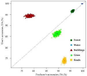
Bayes LULC classification by using 500 sets of bootstrap training samples yielded a total of 500 confusion matrices. The variations of PA and UA are depicted in Figure 9. Both the forest and water LULC classes were associated with high (>95%) classification accuracy and lower uncertainty in PA and UA because of their highly concentrated feature values in the feature space (see Figure 3). By contrast, the feature values of the grass, building, and roads classes were more scattered in the feature space and, therefore, were associated with higher uncertainty in PA and UA. Generally, under the training data uncertainty, the PA and UA of individual LULC classes in our study do not vary by more than 5%. The OA of the 500 sets of confusion matrices varied within only a very small range (89.52%–90.88%). Assuming that the proportions of the training pixels of individual LULC classes are consistent with the a priori probabilities of the individual LULC classes, the global OA and the class-specific global UA can be estimated using the mean values of the OA and class-specific UA of the 500 bootstrap-training-samples-based confusion matrices, respectively. In this study, the global OA was estimated as 90.25%, and the class-specific global UAs of the forest, water, buildings, grass, and roads were estimated as 96.62%, 99.96%, 94.30%, 86.20%, and 73.81%, respectively.
Figure 9. Uncertainties of the producer’s and user’s classification accuracies based on the Bayes LULC classification results derived from 500 sets of bootstrap training samples.
Table 4. Comparison of pixel numbers and areal coverages of the individual LULC classes obtained using original classification and reclassification.
Forest Water Building Grass Roads Original classification
No. of pixels 965,039 163,544 927,127 701,231 860,663
Areal percentage 26.68 4.52 25.63 19.38 23.79
Reclassification
No. of pixels 945,607 164,173 873,766 749,180 884,878
Areal percentage 26.14 4.54 24.15 20.71 24.46
Areal Coverage difference (in km2) 1.9432 −0.0629 5.3361 −4.7949 −2.4215 In a confusion matrix, the class-specific PA and UA, and OA are presented and used to evaluate the LULC classification results. Among these three types of classification accuracy, the PA of a given class is calculated solely on the basis of training pixels of that class. The numbers of training pixels in other classes and their classification do not affect the PA of a given class. By contrast, calculations of the class-specific UA and OA involve the numbers of training pixels that are assigned to all individual classes. Consequently, changing the proportions of the training pixels of individual LULC classes affects the UA and the OA. For example, the training pixels of the buildings and roads LULC classes respectively account for 27% and 17% of all pixels in the training data (see Table 1). Approximately 30% (1331/4595) of the training pixels of the buildings class were misclassified into the roads class, and approximately 93% of the training pixels of the roads class were correctly classified (Table 3), resulting in 73.20% UA for the roads class. Suppose that the proportions of the training pixels of the buildings and roads LULC classes in the original training data set were changed to 32% and 12%, respectively, and the estimated parameters of the multivariate Gaussian distributions of the individual LULC classes remain the same. Under this situation, we can expect that approximately 30% of the training pixels of the buildings class would be misclassified into the roads class, and 93% of the training pixels of the roads class would be correctly classified. However, the UA of the roads class would decrease to below 73.20% because a higher number of pixels from the buildings class would be misclassified into the roads class, and the number of correctly classified pixels of the roads class would be low because of changes in the proportions of training pixels of the buildings and roads classes.
A comparison of the estimates of the class-specific a priori probabilities and the proportions of class-specific training samples in Table 1 reveals that the forest and water classes were given an excess number of training pixels (overrepresented), whereas the grass and roads classes were given insufficient training pixels (underrepresented) in the original training data set. The buildings class was adequately represented in the original training data set. The confusion matrix in Table 3 shows that the pixels that were misclassified into the grass class primarily belong to the forest class. Because the forest and grass LULC classes were respectively over- and underrepresented in the original training data set, we expect that the UA of the grass class (84.83%) in the training-data-based confusion matrix and the global UA of the grass class (86.20%) were underestimated. Similarly, most of the pixels that were misclassified into the roads class actually belong to the buildings class. The roads class was underrepresented in the original training data set, and thus the UA of the roads class (73.20%) in the training-data-based confusion matrix and the global UA of the roads class (73.81%) were also likely to be underestimated.
4.2.2. Pixel-Specific Classification Uncertainty and Identification of Unclassified Pixels
In this study, the pixel-specific CPV was used to characterize the location-specific classification uncertainty. Various measures of classification uncertainty for remote sensing LULC classification have been proposed [40,41]. In the present study, two measures (i.e., the Shannon entropy and
max
The maximum class probability,
p
max, in the CPV of a pixel is used for LULC reclassification. The higher thep
max, the lower the uncertainty in assigning a pixel to the class of the highest class probability. Thus,1
−
p
max indicates possible confusion with other classes. However, the uncertainty measure based onp
max fails to capture the entire distribution of the class probabilities because it considers only the highest class probability in the CPV [41]. By contrast, the Shannon entropy considers all class probabilities and is defined as follows:
=
−
=
Ni i i
p
p
H
1
)
ln
(
ω ω . (5)The entropy can assume a maximum value of lnN if all classes have the same class probabilities. A pixel with
p
max=
1
is associated with zero entropy.Empirical CDFs of the pixel-specific maximum class probability and entropy are shown in Figure 10. Approximately 93% of the pixels in the study area have
p
max=
1
and Shannon entropy H = 0, indicating that using different bootstrap training samples in LULC classification affected the classification results of only 7% of the pixels in the study area. A pixel with zero entropy is always classified into the same LULC class, regardless of the training data uncertainty. However, having zero entropy does not necessarily indicate that the pixel is correctly classified.Figure 10. Empirical cumulative distribution functions of: (a) the maximum class probability (
p
max); and (b) the Shannon entropy (H).Pixels of higher classification uncertainty can be identified using the predetermined threshold values pmax* and
H
* of the maximum class probability and the Shannon entropy, respectively.When the identification of unclassified pixels is desired, these pixels of higher uncertainty can be considered unclassified pixels. Threshold values pmax* and
H
* are associated with a specifiedcutoff probability
p
c (which represents the exceedance probability forH
* and the cumulativeprobability for p*max); that is,
(
pmax< p*max)
= pcProb (6)
(
H
>
H
)
=
p
c*
Figure 10 shows that at a 3% cutoff probability (
p
c=
0
.
03
), the values of pmax* andH
* are 0.9 and 0.325, respectively. Similarly, forp
c=
0
.
01
,p
max* and*
H
are 0.667 and 0.642,respectively. All pixels with a Shannon entropy exceeding
H
* or withp
max value lower than *max
p
are designated as unclassified pixels. The two sets of unclassified pixels, identified byp
*maxand
H
*, respectively, are not identical because a single-value relationship betweenp
max and H does not exist, as depicted in Figure 11. However, a single-value monotonic relationship exists betweenp
max and the minimum conditional entropy, that is,min
(
H
p
max)
, as depicted by the red curve in Figure 11. Thep
max~
min
(
H
p
max)
single-value relationship is expressed as follows:(
) (
)
(
) (
)
< ≤ − − − − < ≤ − − − −= 0.5
3 1 , 2 1 ln 2 1 ln 2 1 5 . 0 , 1 ln 1 ln ) | min( max max max max max max max max max max
max p p p p p
p p p p p p H (8)
The values of
min
(
H
p
max)
and H* are similar for 1 31
max≤
≤ p . For example, given
667 . 0
max=
p , the corresponding values of
min
(
H
p
max)
andH
* are 0.636 and 0.642, respectively.Thus, in practice, substituting
min
(
H
p
max)
forH
* may be convenient, and the correspondingtwo sets of unclassified pixels,
p
*max andmin
(
H
p
max)
, are associated with similar exceedance (orcumulative) probability
p
c. Notably, such unclassified pixels mostly fall near the class boundariesin the feature space and are thus referred to as unclassified pixels identified using the equal-likelihood technique (see Figure 1).
Figure 11. Relationship between the maximum class probability
p
max and Shannon entropy H.4.2.3. Comparison of Unclassified Pixels Identified Using the Chi-square Threshold Technique and Equal-Likelihood Technique
In addition to the equal-likelihood technique, unclassified pixels can also be identified using the following chi-square threshold technique. In this section, we compare the characteristics of unclassified pixels identified using the two methods.
X can be characterized by a multivariate Gaussian distribution, the well-known Hotelling’s
T
2 statistic is defined as follows:(
) (
i i)
T
i
S
X
m
m
X
T
2=
−
−1−
(9)
where mi and Si are, respectively, the sample mean vector and sample covariance matrix of X. Hotelling’s T2 is distributed as a multiple of an F-distribution. However, if
m
i andS
i arecalculated based on random samples of a large sample size (i.e., sample size of the training data in our study), then Hotelling’s T2 can be approximated by a chi-square distribution with k degrees of freedom [42]. The chi-square threshold technique for identifying unclassified pixels can thus be implemented by choosing a threshold value
v
c, which corresponds to an exceedance probabilityc
p
of the chi-square distribution with k degrees of freedom. A value of 0.05 is commonly used forthe exceedance probability
p
c. In this study, digital numbers of three channels (green, red, andNIR) of the ALOS images were selected as classification features; thus,
v
c=
7
.
815
. Pixels with T2values exceeding
v
c fall in the tail of the multivariate Gaussian distribution and are identified asunclassified pixels. In contrast to the equal-likelihood technique, the chi-square threshold technique identifies unclassified pixels without considering possible confusion between land-cover classes.
Unclassified pixels identified using the equal-likelihood technique with p*max =0.9 and those
identified using the chi-square threshold technique with
p
c=
0
.
05
are shown in Figure 12. SpatialFigure 12. (a) Unclassified pixels (white) identified using the equal-likelihood technique with
9 . 0
* max=
p ; (b) unclassified pixels identified using the chi-square threshold technique with
05
.
0
=
cp
; and (c) the Beitou Depot of the Taipei MRT (i.e., the purple-circled area in (b)) (source: https://zh.wikipedia.org/wiki/%E5%8C%97%E6%8A%95%E6%A9%9F%E5%BB%A0).the chi-square threshold technique with pc=0.05; and (c) details of the blue box in (b). Pixels of the Beitou Depot of the Taipei MRT (purple-circled area) were identified as unclassified pixels.
Figure 14. Three-dimensional scatterplots showing: (a) pixels assigned to individual LULC classes (excluding unclassified pixels) through reclassification; (b) unclassified pixels identified using the equal-likelihood technique with pc=0.05; and (c) details of the blue box in (b). Pixels of the Beitou
Depot of the Taipei MRT (purple-circled area) were classified into the buildings class.
5. Conclusions
This study proposes a nonparametric bootstrap resampling approach for assessing uncertainty in LULC classification results. Two techniques for identifying unclassified pixels were also evaluated. The conclusions are as follows:
1. The bootstrap resampling technique can be used to generate multispectral and multiclass bootstrap training data sets.
2. The proposed bootstrap resampling and reclassification approach can be applied for assessing not only the classification uncertainty of bootstrap training samples, but also the class assignment uncertainty of individual pixels.
3. Investigating the effect of the number of bootstrap samples on uncertainty in LULC classification accuracy is advantageous. In our study, 500 sets of bootstrap training samples were sufficient for assessing the uncertainty in the classification accuracy.
4. From the results of the Bayes LULC classification based on 500 sets of bootstrap training samples, the global OA and the class-specific global UA can be estimated as the mean values of the OA and class-specific UA of the 500 bootstrap-training-samples-based confusion matrices, respectively.
with the class-specific a priori probabilities. Training samples that over- or underrepresent certain LULC classes may result in errors in the accuracy of the global UA and OA estimates. 6. Unclassified pixels identified using the chi-square threshold technique represent the outliers of
individual LULC classes but are not necessarily associated with higher classification uncertainty.
7. Unclassified pixels identified using the equal-likelihood technique are associated with higher classification uncertainty and they mostly occur on or near the borders of different land-cover types.
Acknowledgments: We express our gratitude to the Japan Aerospace Exploration Agency for providing the ALOS images through an ALOS Research Agreement (PI-355). We also acknowledge the financial support from a research project grant (NSC 101-2119-M-002-023) from the Ministry of Science and Technology, Taiwan (R.O.C.).
Author Contributions: Ke-Sheng Cheng conceived and designed the research method and framework. Lin-Hsuan Hsiao collected the satellite images and ancillary data, developed computer codes, and conducted the LULC classification. Both authors contributed to the interpretation and evaluation of the results. Ke-Sheng Cheng wrote the paper.
Conflicts of Interest: The authors declare no conflict of interest. The funding sponsors had no role in the design of the study; in the collection, analyses, or interpretation of data; in the writing of the manuscript, and in the decision to publish the results.
Abbreviations
The following abbreviations have been used in this manuscript:
LULC Land-use/land-cover CPV Class-probability vector ALOS Advanced Land Observing Satellite
NIR Near infrared
CDF Cumulative distribution function
UA User accuracy
PA Producer accuracy
OA Overall accuracy
References
1. Price, J.C. Land surface temperature measurements from the split window channels of the NOAA 7 advanced very high-resolution radiometer. J. Geophys. Res. 1984, 89, 7231–7237.
2. Kerr, Y.H.; Lagouarde, J.P.; Imbernon, J. Accurate land surface temperature retrieval from AVHRR data with use of an improved split window algorithm. Remote Sens. Environ. 1992, 41, 197–209.
3. Gallo, K.P.; McNab, A.L.; Karl, T.R.; Brown, J.F.; Hood, J.J.; Tarpley, J.D. The use NOAA AVHRR data for assessment of the urban heat island effect. J. Appl. Meteorol. 1993, 32, 899–908.
4. Wan, Z.; Li, Z.L. A Physics-based algorithm for retrieving land-surface emissivity and temperature from EOS/MODIS data. IEEE Trans. Geosci. Remote Sens. 1997, 35, 980–996.
5. Florio, E.N.; Lele, S.R.; Chang, Y.C.; Sterner, R.; Glass, G.E. Integrating AVHRR satellite data and NOAA ground observations to predict surface air temperature: a statistical approach. Int. J. Remote Sens. 2004, 25, 2979–2994.
6. Cheng, K.S.; Su, Y.F.; Kuo, F.T.; Hung, W.C.; Chiang, J.L. Assessing the effect of landcover on air temperature using remote sensing images—A pilot study in northern Taiwan. Landsc. Urban Plan. 2008, 85, 85–96.
7. Chiang, J.L.; Liou, J.J.; Wei, C.; Cheng, K.S. A feature-space indicator Kriging approach for remote sensing image classification. IEEE Trans. Geosci. Remote Sens. 2014, 52, 4046–4055.
8. Parinussa, R.M.; Lakshmi, V.; Johnson, F.; Sharma, A. Comparing and combining remotely sensed land surface temperature products for improved hydrological applications. Remote Sens. 2016, 8, 162, doi:10.3390/rs8020162.
9. Cheng, K.S.; Wei, C.; Chang, S.C. Locating landslides using multi-temporal satellite images. Adv. Space Res.
10. Teng, S.P.; Chen, Y.K.; Cheng, K.S.; Lo, H.C. Hypothesis-test-based landcover change detection using multi-temporal satellite images–A comparative study. Adv. Space Res. 2008, 41, 1744–1754.
11. Hung, W.C.; Chen, Y.C.; Cheng, K.S. Comparing landcover patterns in Tokyo, Kyoto, and Taipei using ALOS multispectral images. Landsc. Urban Plan. 2010, 97, 132–145.
12. Chen, Y.C.; Chiu, H.W.; Su, Y.F.; Wu, Y.C.; Cheng, K.S. Does urbanization increase diurnal land surface temperature variation? Evidence and implications. Landsc. Urban Plan. 2017, 157, 247–258.
13. Ridd, M.K.; Liu, J.A. Comparison of four algorithms for change detection in an urban environment. Remote Sens. Environ. 1998, 63, 95–100.
14. Sinha, P.; Kumar, L.; Reid, N. Rank-based methods for selection of landscape metrics for land cover pattern change detection. Remote Sens. 2016, 8, 107; doi:10.3390/rs8020107.
15. Cheng, K.S.; Lei, T.C. Reservoir trophic state evaluation using Landsat TM images. J. Am. Water Resour. Assoc. 2001, 37, 1321–1334.
16. Ritchie, J.C.; Zimba, P.V.; Everitt, J.H. Remote sensing techniques to assess water quality. Photogramm. Eng. Remote Sens. 2003, 69, 695–704.
17. Su, Y.F.; Liou, J.J.; Hou, J.C.; Hung, W.C.; Hsu, S.M.; Lien, Y.T.; Su, M.D.; Cheng, K.S.; Wang, Y.F. A multivariate model for coastal water quality mapping using satellite remote sensing images. Sensors 2008,
8, 6321–6339, doi:10.3390/s8106321.
18. Giardino, C.; Bresciani, M.; Villa, P.; Martinelli, A. Application of remote sensing in water resource management: The case study of Lake Trasimeno, Italy. Water Resour. Manag. 2010, 24, 3885–3899, doi:10.1007/s11269-010-9639-3.
19. Joshi, I.; D’Sa, E.J. Seasonal variation of colored dissolved organic matter in Barataria Bay, Louisiana, using combined Landsat and field data. Remote Sens. 2015, 7, 12478–12502, doi:10.3390/rs70912478.
20. Kong, J.L.; Sun, X.M.; Wong, D.W.; Chen, Y.; Yang, J.; Yan, Y.; Wang, L.X. A semi-analytical model for remote sensing retrieval of suspended sediment concentration in the Gulf of Bohai, China. Remote Sens. 2015, 7, 5373–5397, doi:10.3390/rs70505373.
21. Yang, K.; Li, M.; Liu, Y.; Cheng, L.; Huang, Q.; Chen, Y. River detection in remotely sensed imagery using Gabor filtering and path opening. Remote Sens. 2015, 7, 8779–8802, doi:10.3390/rs70708779.
22. Zheng, Z.; Li, Y.; Guo, Y.; Xu, Y.; Liu, G.; Du, C. Landsat-based long-term monitoring of total suspended matter concentration pattern change in the wet season for Dongting Lake, China. Remote Sens. 2015, 7, 13975–13999, doi:10.3390/rs71013975.
23. Qiu, F.; Jensen, J.R. Opening the black box of neural networks for remote sensing image classification. Int. J. Remote Sens. 2004, 25, 1749–1768.
24. Han, M.; Zhu, X.; Yao, W. Remote sensing image classification based on neural network ensemble algorithm. Neurocomputing 2012, 78, 133–138.
25. Mitra, P.; Shankar, B.U.; Pal, S.K. Segmentation of multispectral remote sensing images using active support vector machines. Pattern Recognit. Lett. 2004, 25, 1067–1074.
26. Foody, G.M.; Mathur, A. The use of small training sets containing mixed pixels for accurate hard image classification: Training on mixed spectral responses for classification by a SVM. Remote Sens. Environ. 2006,
103, 179–189.
27. Mountrakis, G.; Im, J.; Ogole, C. Support vector machines in remote sensing: A review. ISPRS J. Photogramm. Remote Sens. 2011, 66, 247–259.
28. Mellor, A.; Haywood, A.; Stone, C.; Jones, S. The performance of random forests in an operational setting for large area sclerophyll forest classification. Remote Sens. 2013, 5, 2838–2856, doi:10.3390/rs5062838. 29. Belgiu, M.; Drăguţ, L. Random forest in remote sensing: A review of applications and future directions.
ISPRS J. Photogramm. Remote Sens. 2016, 114, 24–31.
30. Congalton, R.G. A review of assessing the accuracy of classifications of remotely sensed data. Remote Sens. Environ. 1991, 37, 35–46.
31. Foody, G.M. Thematic map comparison: Evaluating the statistical significance of differences in classification accuracy. Photogramm. Eng. Remote Sens. 2004, 70, 627–634.
32. Foody, G.M. Harshness in image classification accuracy assessment. Int. J. Remote Sens. 2008, 29, 3137–3158. 33. Foody, G.M. Status of land cover classification accuracy assessment. Remote Sens. Environ. 2002, 80, 185–
201.
35. Calibration Result of JAXA Standard Products (As of March 29, 2007). Available online: http://www.eorc.jaxa.jp/en/hatoyama/satellite/data_tekyo_setsumei/alos_hyouka_e.html (accessed on 22 August 2016).
36. Ministry of Interior, Taiwan. Landuse Map, 2009 (A report in Chinese) Available online: http://www.moi.gov.tw/english/ (accessed on 22 August 2016).
37. Efron, B. Bootstrap methods: another look at the jackknife. Ann. Stat. 1979, 7, 1–26.
38. Horowitz, J.L. The bootstrap. In Handbook of Econometrics; Heckman, J.J., Leamer, E., Eds.; North Holland Publishing Company: New York, NY, USA, 2001; Volume 5, pp. 3160–3228.
39. Weber, K.T.; Langille, J. Improving classification accuracy assessments with statistical bootstrap resampling techniques. GISci. Remote Sens. 2007, 44, 237–250.
40. Bo, Y.; Wang, J. A General Method for Assessing the Uncertainty in Classified Remotely Sensed Data at Pixel Scale. In Proceedings of the 8th International Symposium on Spatial Accuracy Assessment in Natural Resources and Environmental Sciences, Shanghai, China, 25–27 June 2008.
41. Loosvelt, L.; Peters, J.; Skriver, H.; Lievens, H.; Van Coillie, F.M.B.; De Baets, B.; Verhoest, N.E.C. Random forests as a tool for estimating uncertainty at pixel-level in SAR image classification. Int. J. Appl. Earth Obs. Geoinf. 2012, 19, 173–184.
42. Liou, J.J.; Wu, Y.C.; Cheng, K.S. Establishing acceptance regions for L-moments based goodness-of-fit tests by stochastic simulation. J. Hydrol. 2008, 355, 49–62.