A Mathematical Problem For Security Analysis Of Hash Functions
And Pseudorandom Generators
Koji Nuida
∗, Takuro Abe
†, Shizuo Kaji
‡, Toshiaki Maeno
§, Yasuhide Numata
¶August 29, 2014
Abstract
In this paper, we specify a class of mathematical problems, which we refer to as “Function Density Problems” (FDPs, in short), and point out novel connections of FDPs to the following two cryptographic topics; theoretical security evaluations of keyless hash functions (such as SHA-1), and constructions of provably secure pseudorandom generators (PRGs) with some enhanced security property introduced by Dubrov and Ishai (STOC 2006). Our argument aims at proposing new theoretical frameworks for these topics (especially for the former) based on FDPs, rather than providing some concrete and practical results on the topics. We also give some examples of mathematical discussions on FDPs, which would be of independent interest from mathematical viewpoints. Finally, we discuss possible directions of future research on other cryptographic applications of FDPs and on mathematical studies on FDPs themselves.
1
Introduction
1.1
Background and related works
It is widely understood that some mathematical problems have been playing indispensable roles in research on cryptography and information security. For instance, the (expected) computational difficulty of integer factorization is the source of security of RSA cryptosystem [10], while the problem of solving multivariate quadratic (MQ) equations has attracted several studies after the development of Matsumoto-Imai cryp-tosystem [7] and its variants, whose constructions are closely related to MQ equations. Hence, posing and studying an interesting mathematical problem which arises in certain cryptographic settings can contribute to the progress of cryptography and information security.
The aim of this paper is to emphasize the significance of a certain mathematical problem, which has connections to the following two major topics in information security; security analysis of keyless hash functions in the real world (such as MD5 and SHA-1), and construction of pseudorandom generators (PRGs) with some enhanced security property. First, we give some descriptions of these two topics.
Security analysis of keyless hash functions. Intuitively, a hash function is a function H:X → Y
from some (finite) setX to another (finite) setY that possesses a certain desirable security property. When we concern efficiency or computability of H, we consider an algorithm that computes H (also denoted by
H) and call it a hash algorithm. One of the standard security requirements for hash functions is collision resistance, which informally means that it is difficult to find a collision pair (x1, x2) forH, i.e.,x1̸=x2∈X
satisfyingH(x1) = H(x2). Hash functions have been playing central roles in various information security
∗Combutational Biology Research Center (CBRC) / Research Institute for Secure Systems (RISEC), National Institute of
Advanced Industrial Science and Technology (AIST), Japan ([email protected])
†Department of Mechanical Engineering and Science, Kyoto University, Japan ([email protected]) ‡Department of Mathematical Sciences, Faculty of Science, Yamaguchi University, Japan ([email protected]) §Department of Mathematics, Meijo University, Japan ([email protected])
applications, and secure hash functions for real-life applications are usually expected to possess the collision resistance property.
However, most of the preceding successful studies that show security of hash functions actually dealt with keyed hash functions (or hash families); intuitively, a family of hash functions Hk parameterized by
a keyk is called collision resistant if, for any (efficient) adversary, the attack to find a collision pair ofHk
fails with high probability for a randomly chosen keyk. Several constructions of keyed hash functions have been proposed so far (e.g., [3]). The above security notion of keyed hash functions can be interpreted as allowing one to (randomly) choose a concrete instance Hk of the hash family after an adversary is given.
In contrast, in most of real-life applications, the concrete instance of hash algorithms is specified first (for example, by a standardization), and then an adversary can try to attack the fixed hash algorithm. This reversal of order causes a crucial difficulty in guaranteeing (or even formalizing in a reasonable manner) security of a keyless hash algorithmH, as (unless the trivial situation where the domain ofH is not larger than the image ofH) there does alwaysexist a collision pair (x1, x2) forH and any adversary (existing in theory) who innately knows the pair (x1, x2) is obviously able to efficiently attack the fixed hash algorithm
H. In fact, even an instance of standardized (or de facto standard) hash algorithms, whose security must be evaluated well before the standardization, has been suffered from feasible attacks (e.g., [12]). In this paper, we try to propose a theoretical and unified way to say something, preferably affirmative, about security of a concrete (keyless) instance of hash algorithms.
For related works, Rogaway [11] gave a detailed observation about the difference between “inexistence of effective attack algorithms” and “lack of knowledge on construction of effective attack algorithms” for keyless hash algorithms. He emphasized the difference of the two situations (by the term “human ignorance”), and discussed how to prove security of a cryptographic protocol by reducing the security into “lack of knowledge on concrete attacks” on the hash algorithm internally used by the protocol. However, he did not discuss how to theoretically evaluate security of keyless hash algorithms themselves, which we study in this paper. On the other hand, in this paper we adopt concrete security formulation rather than asymptotic one; while some observation for security of keyless hash algorithms in asymptotic security formulation is also given in Rogaway’s paper.
Construction of enhanced PRGs. A PRG is an algorithm G:S → X with (finite) set S of inputs (seeds) and (finite) output setX with the property that, when a seeds∈S is chosen uniformly at random, the output G(s)∈X of Gis also “random” in some sense. Conventionally, the meaning of “randomness” here is formulated by using the notion of distinguisher, which is an algorithm D: X → {0,1} with 1-bit output and the input set being the output setX ofG. In this paper we adopt concrete security formulation rather than asymptotic one, in which case the security requirement for PRGs can be formulated as (T, ε )-security; namely,Gis called (T, ε)-secure[5] if, for any distinguisherDforGwith (time) complexity bounded byT, the statistical distance between the output distribution D(G(US)) of D with input given by Gwith
uniformly random seeds∈S (referred to as “pseudorandom input”) and the output distributionD(UX) of
D with uniformly random input x∈X (referred to as “random input”) is bounded by ε. (Intuitively, any suchD cannot distinguish the random elementxand the pseudorandom elementG(s) inX with significant advantage.) There are a large number of constructions of PRGs, most of which are provably secure (possibly in asymptotic security formulation) under standard computational assumptions (e.g., [2, 5]).
On the other hand, in a preceding work of Dubrov and Ishai [4], an enhanced notion for PRGs, called
pseudorandom generators that fool non-boolean distinguishers (nb-PRGs, in short), was proposed. This notion is obtained by allowing the distinguishersD in the above security notion to have larger output sets; namely, G is called (T, n, ε)-secure if, for any “non-boolean” distinguisher D: X → Y for G with (time) complexity bounded by T and output set Y of size at mostn, the statistical distance between the output distributions of D with random and pseudorandom inputs is bounded by ε. Dubrov and Ishai showed interesting applications of nb-PRGs, e.g., secure pseudorandomization of a certain kind of information-theoretically secure protocols without any restriction on computational complexity of the adversary’s attack algorithm.
Indeed, to the authors’ best knowledge, the only constructions of nb-PRGs proposed so far are ones in the original paper [4], which are based on certain less standard computational assumptions. Hence it will be fruitful if we can give some results implying thatany usual PRG (with some parameter) is also an nb-PRG (with a possibly different parameter). In fact, a straightforward implication has been mentioned in [4], but this is far from being efficient (i.e., to obtain nb-PRGs with reasonable security parameters, the original PRGs are required to have somewhat impractical security parameters). In this paper, we try to establish a more efficient implication result.
1.2
Our contributions, and organization of this paper
In Section 2, we propose a class of mathematical problems, which we refer to as “Function Density Problems”. Intuitively, this problem is to evaluate the possibility of close approximations of arbitrary functions by using some “easily describable (or analyzable)” functions.
Then we introduce motivating applications of Function Density Problems to two topics in information security. First, in Section 3, we discuss theoretical analysis of collision resistance of keyless hash algorithms. We give an abstract framework for attacking a given hash algorithm by using known attacks on some other “easily breakable” hash algorithms. In the framework, it is essential to evaluate how closely a target hash algorithm can be approximated by “easily breakable” hash algorithms; thus Function Density Problems play a significant role in the security evaluation of hash algorithms.
Secondly, in Section 4, we study an enhanced security notion for PRGs (called nb-PRG) introduced by Dubrov and Ishai [4]. We give some implication results showing that any secure PRG with some parameter is also a secure nb-PRG with somewhat modified security parameter. In the results, the overheads in the bounds of (time) complexity and of advantages for the distinguishers are in trade-off relations, and Function Density Problems can be applied to evaluate to what extent the trade-off will be improved by our proposed result.
Then, in order to arise some image or intuition of how Function Density Problems can be mathematically studied, in Section 5 we give some concrete examples of mathematical discussions on Function Density Problems themselves, using combinatorial and geometric arguments and techniques in Gr¨obner bases. In particular, we deal with special cases where the set of “easily describable (or analyzable)” functions forms a linear subspace (related to low-degree boolean functions, perfect linear codes and Reed–Solomon codes), which would be of independent interest from mathematical viewpoints.
Finally, in Section 6 we give a concluding remark, which includes discussions on further possible appli-cations of Function Density Problems in information security, and on possible directions of future research on Function Density Problems themselves.
2
Function Density Problems
In this section, we specify a class of mathematical problems, which we call Function Density Problems
(FDPs) in this paper. As the class of FDPs in a most general form will include too various problems to obtain meaningful insights for their properties, it is significant to restrict the class suitably according to each situation under consideration. Relations of FDPs to some concrete topics in cryptography will be shown in the following sections.
We give a general description of our problem:
Definition 1 (Function Density Problems). LetC be a set of some functions, and letC′ be a subset ofC. Letd(·,·) be a distance function for the pairs of functions inC. In this setting, we define aFunction Density Problem to be a problem of estimating the following quantity:
r(C,C′) := sup{d(f,C′)|f ∈ C} , (1)
Among very various situations covered by Definition 1 (where C in fact need not even to be a set of functions), in the applications of FDPs discussed in this paper we will focus on the following typical cases:
Definition 2(Function Density Problems – typical cases). LetCbe the set of all functionsf:X →Y from a given finite setX to a given finite setY. Let C′⊂ C. For anyf, g∈ C, we define the distance betweenf
andg by
dH(f, g) :=|{x∈X |f(x)̸=g(x)}| . (2)
In this setting, aFunction Density Problem is a problem of estimating the quantityr(C,C′) defined by (1) withd(·,·) =dH(·,·).
In the case of Definition 2, the “sup” and “inf” in Definition 1 can be simply replaced with “max” and “min”, respectively. Moreover, the distance defined by (2) coincides with the (generalized) Hamming distance when members of C are identified with sequences of length |X| over the alphabet Y in a natural manner. Note that the quantityr(C,C′) can be regarded as a special case of so-called Hausdorff distance for two subsets of a metric space, which would support that it is reasonable to considerr(C,C′).
An intuitive explanation of a motivation for the above definition is as follows. Given a setCof functions, a subsetC′consists of members ofCwhich are in some sense “easily analyzable” or “with simple descriptions”. The distance d(f, g) measures how two functionsf andg are similar. Then the quantityd(f,C′) evaluates how accurately a functionf ∈ C can be approximated by an “easy” function inC′, and the quantityr(C,C′) evaluates how densely the “easy” functions distribute among the entire setC. In other words, whenr(C,C′) is revealed to be small, it shows potential availability of a close approximation of any member ofCby an “easy” function inC′. For example, in the case of Definition 2, any function f ∈ C can in principle be converted into some function g ∈ C′ by changing the values f(x) for at most r(C,C′) points x∈X. (We emphasize that it does not mean that a close approximation of f by a function in C′ can be efficiently computable. Such a difference between existence and efficient computability is also relevant to a preceding observation for “human ignorance” by Rogaway [11].)
3
Hash Functions and FDPs
In this section, we point out a relation of FDPs introduced in Section 2 to security analysis of keyless hash functions. Here we propose a new framework for theoretical security evaluation of keyless hash functions based on FDPs. Although theoretical security evaluation of keyless hash functions is evidently an extremely difficult problem and our proposed framework is unfortunately not yet practical, we hope that our framework can be a clue to this problem.
We consider a keyless hash function H:X →Y with possibly large but finite domainX and relatively small (finite) rangeY. Among the major security requirements for hash functions, we focus on the collision resistance of H; we discuss how it is difficult to find a collision pair (x1, x2) for H (recall that (x1, x2) is called a collision pair forH if we havex1, x2∈X, x1̸=x2 andH(x1) =H(x2)). To show the relevance of FDPs to this problem, first we give a somewhat informal description of an abstract “typical” strategy for finding a collision pair:
1. Construct a close approximation H′:X → Y of H in such a way that collision pairs forH′ can be found with reasonable computational time.
2. Find randomly a collision pair (x′1, x′2) forH′.
3. Construct from (x′1, x′2) a candidate (x1, x2) of a collision pair forH (in the simplest case, we just set (x1, x2) = (x′1, x′2)).
4. Check if (x1, x2) is a collision pair ofH; if it is indeed a collision pair ofH, then output (x1, x2) and stop the process.
Intuitively, the number of iterations in the above strategy before finding a collision pair for H would be expected to be small if the approximationH′ is sufficiently close toH (see Lemma 1 below for a quantitative expression of this expected tendency). Hence security of a hash algorithmH against such an attack strategy is related to the possibility of finding its close approximation.
More precisely, we set (x1, x2) = (x′1, x′2) in the above strategy for simplicity. We consider the case
of Definition 2, and let C′ be a subset of C with the property that any hash function H′ in C′ admits an efficient attack (finding a collision pair) by a certain known attack strategy. In the above attack strategy, the approximationH′ forH specified in Step (1) is supposed to be chosen fromC′. Now we have the following lemma:
Lemma 1. Suppose thatH andH′are functionsX →Y with|Y|=n≥2, anddH(H, H′) =d,0< d <|X|.
Then the probability that a collision pair for H′, which is chosen uniformly at random from the set of all collision pairs for H′, is also a collision pair forH is not lower than
2α0|X| −n(α0+ 1)α0−2dα0
2α0|X|+ 2d|X| −n(α0+ 1)α0−2dα0−d2−d , (3)
where α0 =⌊(|X| −d−1)/n⌋. Moreover, when |X| ≥ d+ (n−1)2, the value in (3) is getting larger asd
becomes smaller.
A proof of Lemma 1 will be provided in the last of this section. Now let us imagine the following situation. Two candidate sets C1,C2 for a new standard hash function are given, and we can specify subsetsC1′ ⊂ C1
and C′2⊂ C2 in such a way that each Ci′ (i= 1,2) consists of some hash functions for which collision pairs
can be found in reasonable computational time by using some known techniques. We suppose thatr(C1,C1′)
is significantly small andr(C2,C2′) is significantly large. Then any hash functionH chosen fromC1 can be
potentially attacked by just finding a close approximation H′ ∈ C1′ of H (using some expert’s sixth sense, for example) and applying the above attack strategy combined with known collision finding techniques. On the other hand,C2contains at least one hash functionH for which the above attack strategy combined with
any known collision finding technique will not succeed. This would suggest that it can be potentially safer to choose a new hash function fromC2rather thanC1, as we already know the potential attack on any hash
function inC1 but not the same forC2.
The authors hope that studies of FDPs can contribute to security analysis of keyless hash functions in the above manner, though how to specify the subsetC′ in practical cases is of course a big problem to be concerned. One may also feel that it seems infeasible to compute the quantity r(C,C′) for practical classes of hash functions; even if so, some estimate of a bound or tendency ofr(C,C′) would still give us an insight into the security level of those hash functions.
Remark 1. Here we notice that, although we have focused on the collision resistance in the above argument, a similar idea would also be applicable to other security notions for keyless hash functions, such as the (second) preimage resistance.
To conclude this section, we give a proof of Lemma 1.
Proof of Lemma 1. We write (m)2 := m(m−1) for any integer m. Put Y := {y1, . . . , yn}, and for each
1≤i≤n, put
ai:=|{x∈X |H′(x) =yi}|, bi:=|{x∈X|H(x)̸=H′(x) =yi}| . (4)
Moreover, put
φ1(⃗a;⃗b) :=
n ∑
i=1
(ai)2, φ2(⃗a;⃗b) :=
n ∑
i=1
(ai−bi)2 , (5)
where⃗a:= (a1, . . . , an) and⃗b:= (b1, . . . , bn). Then the number of collision pairs forH′ isφ1(⃗a;⃗b), while the
number of collision pairs for H is at leastφ2(⃗a;⃗b). Therefore the probability specified in the statement of
Lemma 1 is at least
φ(⃗a;⃗b) := φ2(⃗a;⃗b)
From now, we give a lower bound for the values ofφunder the following conditions implied by the definitions: 0≤bi≤aifor eachi,
∑n
i=1ai=|X|, and ∑n
i=1bi =d. For the purpose, we show the following two lemmas:
Lemma 2. In the above setting, if the minimum value of the function φ is attained by ⃗a and⃗b, then we havebi>0 for a unique indexi, andai−bi≥aj for every index j̸=i.
Proof. If we havei̸=j andbi, bj>0, and we supposeai≤aj by symmetry, then we have (
(ai−1)2+ (aj+ 1)2
)
−((ai)2+ (aj)2
)
= 2(aj−ai+ 1)>0 , (7)
therefore the value ofφ1increases when ai,aj,bi andbj are replaced withai−1,aj+ 1, bi−1 and bj+ 1,
respectively. On the other hand, the value ofφ2 is not changed by this replacement. Therefore the value of
φis decreased by this replacement, contradicting the assumption on the choice of⃗aand⃗b. Hence an index
iwithbi>0 is unique, thereforebi=d. Similarly, ifj ̸=i andai−bi< aj, then we have (
(ai−bi+ 1)2+ (aj−1)2
)
−((ai−bi)2+ (aj)2
)
= 2(ai−bi−aj+ 1)≤0 , (8)
with equality holding when and only whenai−bi=aj−1. This implies that the value ofφat the⃗aand⃗b
is larger than or equal to the value ofφwith bi andbj (= 0) being replaced withbi−1 and 1, respectively,
where the equality holds if and only ifai−bi =aj−1. As the former value is assumed to be the minimum,
the equality condition ai−bi = aj−1 should hold. Moreover, if bi−1 > 0, then the latter value of φ
(which is now equal to the former) cannot be the minimum by the above argument, which also leads to a contradiction. Hence we havebi= 1 (therefored= 1) andai=aj. Now we have
(
(ai+ 1)2+ (aj−1)2
)
−((ai)2+ (aj)2
)
= 2(ai−aj+ 1)>0 . (9)
This implies that the value ofφwill decrease whenaiandaj are replaced withai+ 1 andaj−1, respectively,
contradicting the assumption that the former value is the minimum. Hence we haveai−bi ≥aj for every
j̸=i, concluding the proof of Lemma 2.
Lemma 3. In the above setting, if the minimum of the function φ is attained by⃗a and⃗b, then we have
|ai−aj| ≤1for any pair of indices i̸=j satisfying bi=bj = 0.
Proof. Assume contrary thatai−aj ≥2 for such a pair of indices i̸=j. For ℓ∈ {1,2}, let αℓ denote the
value ofφℓ at the⃗aand⃗b, and let βℓ denote the value ofφℓ withai andaj being replaced withai−1 and
aj+ 1, respectively. Then we have β1−α1 =β2−α2 = 2(aj−ai+ 1)<0. On the other hand, for the
unique indexi′ withbi′ >0 (see Lemma 2), we haveai′ ≥bi′+ai ≥bi′+aj+ 2≥2 by the assumption and
Lemma 2, thereforeα1> α2. Now we present the following lemma, which is proven by an easy calculation:
Lemma 4. Ifp > q≥0 andr >0, then q/p <(q+r)/(p+r).
By using this lemma, we have
α2 α1
= β2−2(aj−ai+ 1)
β1−2(aj−ai+ 1)
> β2 β1
, (10)
contradicting the assumption thatα2/α1 is the minimum of the value ofφ. Hence Lemma 3 holds.
By Lemma 2 and Lemma 3, the points ⃗a and⃗b that attain the minimum of φ satisfy the following conditions: bi >0 for a uniquei, and there is an integerαsatisfying thatai−bi≥α+ 1 andaj∈ {α, α+ 1}
for everyj̸=i. Note that thisαcan be taken asα≥0; indeed, this is obvious if someajwithj̸=iis positive,
while the remaining possibility thataj = 0 for every j ̸=i allows us to chooseα= 0 asai =|X|> d=bi
ai=|X|−(n−1)α−k, whilebi=d, therefore the conditionai−bi≥α+ 1 implies thatk≤ |X|−nα−d−1.
Now we write the values ofφ1 andφ2 in this case asφ1(α, k) andφ2(α, k), respectively. Then we have
φ1(α, k) =k(α+ 1)2+ (n−1−k)(α)2+ (ai)2 , φ2(α, k) =k(α+ 1)2+ (n−1−k)(α)2+ (ai−d)2 ,
(11)
thereforeφ1(α, k)−φ2(α, k) = 2dai−d2−d. Now by Lemma 4, we have
1−φ2(α, k)
φ1(α, k)
=2dai−d
2−d φ1(α, k)
≤ 2dai−d2−d+ 2d((n−1)α+k)
φ1(α, k) + 2d((n−1)α+k)
= 2d|X| −d
2−d
k(α+ 1)2+ (n−1−k)(α)2+ (ai)2+ 2d(n−1)α+ 2dk
(12)
(note that 2d((n−1)α+k)≥0 asα≥0). Letψ(α, k) denote the denominator of the right-hand side. Then, by virtue of the property ∂k∂ ai=−1, we have
∂
∂kψ(α, k) = (α+ 1)2−(α)2−(2ai−1) + 2d= 2α−2ai+ 1 + 2d <0 (13)
(note that ai−d≥α+ 1), therefore ψ(α, k) is decreasing as k is increasing. On the other hand, we have
ψ(α, n−1) =ψ(α+ 1,0). Now note thatα≤(|X| −d−1)/nas 0≤k≤ |X| −nα−d−1. This implies that
ψ(α, k) takes the minimum value atα=⌊(|X| −d−1)/n⌋=α0andk=k0:=|X| −nα0−d−1 (note that
k0≤n−1). Moreover, we haveai =α0+d+ 1 ifα=α0and k=k0. Hence a straightforward calculation
shows that
1−φ2(α, k)
φ1(α, k) ≤
2d|X| −d2−d ψ(α0, k0)
= 2d|X| −d
2−d
2α0|X|+ 2d|X| −n(α0+ 1)α0−2dα0−d2−d ,
(14)
therefore
φ2(α, k) φ1(α, k)≥1−
2d|X| −d2−d
2α0|X|+ 2d|X| −n(α0+ 1)α0−2dα0−d2−d
= 2α0|X| −n(α0+ 1)α0−2dα0
2α0|X|+ 2d|X| −n(α0+ 1)α0−2dα0−d2−d ,
(15)
which proves the lower bound (3) in the statement of Lemma 1.
Finally, suppose that d≥2, and letη1(d) andη2(d) denote the denominator and the numerator in (3),
respectively. For any valuexdepending ond, let ∆[x] temporarily denote the value ofxatd−1 minus the value ofxatd. Then we have ∆(−d2−d) = 2d, therefore
∆[η2(d)] = ∆[2α0|X| −n(α0+ 1)α0−2dα0] ,
∆[η1(d)] = ∆[2α0|X| −n(α0+ 1)α0−2dα0]−2|X|+ 2d <∆[η2(d)] .
(16)
Moreover, we have ∆[α0] ∈ {0,1}, and if ∆[α0] = 0, then ∆[η2(d)] = 2dα0 > 0. On the other hand, if ∆[α0] = 1, then we have
∆[(α0+ 1)α0] = (α0+ 2)(α0+ 1)−(α0+ 1)α0= 2(α0+ 1) ,
∆[2dα0] = 2(d−1)(α0+ 1)−2dα0= 2d−2α0−2 , (17)
therefore
∆[η2(d)] = 2|X| −2n(α0+ 1)−2d+ 2α0+ 2
= 2|X| −2(n−1)α0−2n−2d+ 2
≥2|X| −2(n−1)|X| −d−1
n −2n−2d+ 2
= 2
n
(
|X| −d+ 2n−1−n2)≥0
(where we used the assumption|X| ≥d+ (n−1)2). Now by Lemma 4, we have
η2(d−1)
η1(d−1)
= η2(d) + ∆[η2(d)]
η1(d) + ∆[η1(d)]
≥ η2(d)
η1(d) + ∆[η1(d)]−∆[η2(d)]
> η2(d) η1(d)
. (19)
Hence the proof of Lemma 1 is concluded.
4
PRGs and FDPs
As our second application of FDPs, in this section we present some results which prove that any (computa-tionally indistinguishable) PRG with some parameter is also an nb-PRG with a (possibly different) specified parameter. The concrete relations between parameters for an algorithm as a PRG and as an nb-PRG, respectively, will be determined by applying FDPs.
First we recall the security notion for PRGs. We emphasize that, for the sake of simplicity, here we adopt definitions in forms of concrete security rather than asymptotic security. LetUX denote the uniform
probability distribution over a finite setX.
Definition 3 (see e.g., [5]). LetG:S →X be an algorithm with finite input setS and finite output setX. Given parameters T ≥0 andε ≥0, Gis called a (T, ε)-secure pseudorandom generator (PRG) if, for any algorithm (called adistinguisher)D:X→ {0,1}with time complexity bounded byT, we haveAdvD(G)≤ε
whereAdvD(G) denotes theadvantage ofDdefined by
AdvD(G) :=|P r[D(UX) = 1]−P r[D(G(US)) = 1]| . (20)
Let ∆(P1, P2) denote the statistical distance of two probability distributionsP1, P2 over the same finite setZ defined by
∆(P1, P2) := 1 2
∑
z∈Z
|P r[P1=z]−P r[P2=z]| (21)
= max
E⊂Z|P r[P1∈E]−P r[P2∈E]| . (22)
Then the advantageAdvD(G) of a distinguisher D defined above is equal to ∆(D(UX), D(G(US))), as both
D(UX) and D(G(US)) are probability distributions over{0,1}. This interpretation of the advantage gives
us a motivation to enhance the above security notion of PRGs, as in the following definition introduced by Dubrov and Ishai [4] (with slightly different formulation):
Definition 4 ([4]). Let G: S → X be an algorithm with finite input set S and finite output set X. Given parameters T ≥ 0, ε ≥ 0 and an integer n ≥ 2, G is called (T, n, ε)-secure if, for any algorithm (distinguisher)D:X → {0,1, . . . , n−1}with time complexity bounded byT, we haveAdvD(G)≤εwhere
we put AdvD(G) := ∆(D(UX), D(G(US))). Such an algorithm G is called a PRG that fools non-boolean
distinguishers (nb-PRG, in short).
Our proposal here is to establish a general theorem of the following form: Any (T′, ε′)-secure PRG is also a (T, n, ε)-secure nb-PRG, where the parameters T′ and ε′ as a usual PRG are determined by T, n
andεin a certain manner. Such an implication result is evidently meaningful, as it enables us to convert a large number of existing PRGs under standard assumptions into nb-PRGs. In fact, an implication relation as above has been mentioned (without proof) in [4]. Our aim here is to improve the preceding relation by introducing the idea of FDPs.
The above-mentioned relation is derived from the first expression (21) of statistical distance, in the following manner (which refers to a description in [9]). We introduce some notations. PutY :={0,1, . . . , n−
1} for simplicity. For any subsetZ⊂Y, letχZ:Y → {0,1} denote the characteristic function ofZ defined
byχZ(x) = 1 ifx∈Z andχZ(x) = 0 if x∈Y \Z. We write χz =χ{z} for simplicity whenZ ={z}. In
this setting, for any PRGG:S→X and any non-boolean distinguisherD:X →Y, the statistical distance ∆(D(UX), D(G(US))) is equal to
1 2
∑
y∈Y
|P r[D(UX) =y]−P r[D(G(US)) =y]|
= 1 2
∑
y∈Y
|P r[χy◦D(UX) = 1]−P r[χy◦D(G(US)) = 1]|
= 1 2
∑
y∈Y
Advχy◦D(G) ,
(23)
whereχy◦D denotes an algorithm performed by first executing the distinguisherDand then evaluating the
output ofD by the functionχy. An important property is thatχy◦D is a 1-bit output algorithm, therefore
it can be regarded as a distinguisher for the PRGG. This implies that, to show that a (T′, ε′)-secure PRGG
is also a (T, n, ε)-secure nb-PRG, it suffices to choose the parameters asT′=T+δ1andε′ = 2ε/n, whereδ1
is the maximum of the overhead in computational complexity of composing someχy (y∈Y) toD (usually,
δ1 can be set to be almost zero in practical situations). In other words, we have the following proposition (which has been mentioned in [4]):
Proposition 1. In this setting, any(T +δ1,2ε/n)-secure PRG is also(T, n, ε)-secure, where the quantity
δ1 is defined in the above manner.
A drawback of this result is that, in practical applications the parameter n (which is relevant to the allowable input size for an adversary against a protocol under consideration) should frequently be large, which makes the overhead in a bound of advantage in Proposition 1 too heavy. We try to resolve the drawback by improving or modifying the above result.
Our first idea is to use the second expression (22) of statistical distance instead of the first one (21) used in the preceding argument. Namely, in the same setting as above, the statistical distance ∆(D(UX), D(G(US)))
is equal to
max
Z⊂Y|P r[D(UX)∈Z]−P r[D(G(US))∈Z]|
= max
Z⊂Y|P r[χZ◦D(UX) = 1]−P r[χZ◦D(G(US)) = 1]|
= max
Z⊂YAdvχZ◦D(G) .
(24)
In the same way as Proposition 1, the above argument implies the following result:
Proposition 2. In this setting, any(T+δ2, ε)-secure PRG is also(T, n, ε)-secure, whereδ2is the maximum
of the overhead in computational complexity of composing someχZ withZ ⊂Y :={0,1, . . . , n−1} toD.
heavy, as the setY (of somewhat large size) may contain an extremely complicated subsetZ, for which the computation ofχZ would be inefficient.
From now, we try to improve the above-mentioned trade-off between overheads for bounds of advantage and of computational complexity, by applying the idea of FDPs. PutY :={0,1, . . . , n−1}as above, and let
Cbe the set of characteristic functionsχZ:Y → {0,1}for subsetsZ⊂Y, and letd=dH(see (2)). Then for χY1, χY2 ∈ C,dH(χY1, χY2) is equal to the size of the symmetric difference Y1⊖Y2:= (Y1\Y2)∪(Y2\Y1) of two subsetsY1andY2. Now we fix a subsetC′ofC. Letδ3be the maximum of the overhead in computational
complexity of composing someχZ∈ C′ toD. Moreover, we putr:=r(C,C′) for simplicity. Then we have the
following result (we notice that, whenC′ ={χ∅}, the theorem gives almost the same result as Proposition 1):
Theorem 1. In the above situation, letδ1be as specified in Proposition 1. IfG:S→X is(T+δ1, ε1)-secure and(T+δ3, ε3)-secure, thenG is also(T, n, rε1+ε3)-secure.
Proof. For each distinguisher D: X → Y := {0,1, . . . , n−1}, we write µ(Z) := P r[D(UX) ∈ Z] and
µ′(Z) :=P r[D(G(US))∈Z] for a subsetZ⊂Y. LetY0 be a subset ofY that attains the maximum of the
second expression (22) of the statistical distance;
∆(D(UX), D(G(US))) =|µ(Y0)−µ′(Y0)| . (25)
Note thatY0can be chosen in such a way thatµ(Y0)−µ′(Y0)≥0 (if this inequality fails, useY \Y0instead
ofY0), therefore
∆(D(UX), D(G(US))) =µ(Y0)−µ′(Y0) . (26)
Moreover, by the definition of r, there is a subset Y1 ⊂ Y satisfying that χY1 ∈ C′ and dH(χY0, χY1) =
|Y0⊖Y1| ≤r. Now we have
ν(Y0)−ν(Y1) =ν(Y0\Y1)−ν(Y1\Y0) for eachν ∈ {µ, µ′} , (27)
therefore we have
(µ(Y0)−µ′(Y0))−(µ(Y1)−µ′(Y1))
= (µ(Y0)−µ(Y1))−(µ′(Y0)−µ′(Y1))
= (µ(Y0\Y1)−µ′(Y0\Y1))−(µ(Y1\Y0)−µ′(Y1\Y0)) .
(28)
Moreover, the right-hand side is equal to
∑
y∈Y0\Y1
(µ({y})−µ′({y}))− ∑
y∈Y1\Y0
(µ({y})−µ′({y}))
≤ ∑
y∈Y0⊖Y1
|µ({y})−µ′({y})|
= ∑
y∈Y0⊖Y1
|P r[χy◦D(UX) = 1]−P r[χy◦D(G(US)) = 1]|
= ∑
y∈Y0⊖Y1
Advχy◦D(G) .
(29)
Now ifD has computational complexity bounded by T, then the assumption onGand the definition of δ1
imply that ∑
y∈Y0⊖Y1
Advχy◦D(G)≤
∑
y∈Y0⊖Y1
ε1=|Y0⊖Y1| ·ε1≤rε1 . (30)
Summarizing, we have
This and (26) implies that
∆(D(UX), D(G(US)))
= (µ(Y0)−µ′(Y0))−(µ(Y1)−µ′(Y1)) + (µ(Y1)−µ′(Y1))
≤rε1+ (P r[D(UX)∈Y1]−P r[D(G(US))∈Y1])
≤rε1+|P r[χY1◦D(UX) = 1]−P r[χY1◦D(G(US)) = 1]| =rε1+AdvχY1◦D(G)≤rε1+ε3 ,
(32)
concluding the proof of Theorem 1.
Regarding the relation between parameters in Theorem 1, first note that it is natural by the definitions to expect thatδ1≤δ3, which allows us to suppose thatε1≤ε3. Now let us imagine the following situation:
We can find an appropriate subset C′ ⊂ C in such a way that every characteristic functionχZ ∈ C′ has low
computational complexity and the quantityr:=r(C,C′) is small. In this case,δ3 can be small as well as r,
and it would make the implication relation given by Theorem 1 more efficient than those in Propositions 1 and 2, therefore the above-mentioned trade-off is improved. Hence a study of FDPs (in particular, those for functions with 1-bit output sets) will contribute to establish a better relation between PRGs and nb-PRGs.
Remark 2. We mention that, for the two applications of FDPs discussed in the last two sections, a kind of “risk-hedging” relation exists as follows. Namely, if we find that the quantity r(C,C′) tends to be large in general, then it would support the argument in Section 3 to show that keyless hash functions under consideration would have better security. On the other hand, if we find that the quantityr(C,C′) tends to be small in general, then it would support the argument in Section 4 to show that overheads in parameters for nb-PRGs compared to PRGs would be practically small.
At the last of this section, we give an example of the possible choices of the distinguished subset C′ of
C. We consider the case thatn= 2ℓfor an integer ℓ; now the setY is identified with{0,1}ℓ via the binary expression of integers, and each elementχZ ofCis regarded as a boolean function{0,1}ℓ→ {0,1}withℓ-bit
input. In this setting, our task is to find a setC′of “easy” boolean functions withℓ-bit inputs, for which each function inC can be closely approximated by some function inC′. Here we consider ℓ-variabledisjunctive normal form (DNF)formulae; recall that aliteral isyi or yi (logical NOT ofyi) where y1, . . . , yℓ ∈ {0,1}
are input bits for a boolean function, a term is a logical AND of literals, and a DNF formula is a logical OR of terms. The number of terms in a DNF formula is called thesize of the formula. It is straightforward to show that anyℓ-bit input boolean function is equivalent to some DNF formula of size 2ℓ. Below we will
define C′ to be the set of (ℓ-bit input) boolean functions which are either a logical XOR of at most ℓ DNF formulae of size significantly smaller than 2ℓ, or the logical NOT of such a function. Now the functions inC′
is expected to be easier to compute than general boolean functions, hence the overheadδ3 in the bound for the distinguisher’s computational complexity in Theorem 1 would be significantly better (i.e., smaller) than its counterpartδ2in Proposition 2, as desired.
Before specifying the sizes of the DNF formulae in the choice of C′, first we give the following argument. A boolean function f: {0,1}ℓ → {0,1} is called monotone, if yi ≤ yi′ for every i ∈ {1, . . . , ℓ} implies
f(y1, . . . , yℓ)≤ f(y′1, . . . , yℓ′). We note that χZ ∈ C is monotone if and only ifZ ⊂ {0,1}ℓ is a filter (i.e.,
upper-closed set) of theℓ-dimensional lattice{0,1}ℓ. Then we have the following result:
Lemma 5. Any χZ ∈ C with ⃗0 := (0,0, . . . ,0) ̸∈ Z can be expressed as the logical XOR of at most ℓ
monotone boolean functions.
Proof. Let Z1 denote the filter of {0,1}ℓ generated by the minimal (with respect to the order of {0,1}ℓ)
elements of Z. Then we have Z ⊂ Z1 and χZ = χZ1 ⊕χZ1\Z where ⊕ denotes the logical XOR. The claim holds if Z1\Z = ∅. On the other hand, if Z1\Z ̸=∅, then we iterate the process to decompose χZ1\Z. As the minimum weight of minimal elements ofZ1\Z is strictly larger than the minimum weight of minimal elements of Z, and⃗0̸∈Z by the assumption, the process terminates with at mostℓ steps, giving the decompositionχZ =χZ1⊕ · · · ⊕χZℓ′ with Zi being filters of {0,1}
ℓ, 1≤i ≤ℓ′ ≤ℓ. Hence the claim
By the lemma, for any χZ ∈ C, either χZ or χZ =χ{0,1}ℓ\Z can be expressed as the logical XOR of
at most ℓ monotone boolean functions. On the other hand, for each of these monotone functions, recently Blais, H˚astad, Servedio and Tan [1] showed the following result:
Proposition 3 (See [1]). For any 0< η <1, every ℓ-bit input monotone boolean function f can be approx-imated by a DNF formula g of size 2ℓ−Ω(√ℓ) satisfying that d(f, g)≤η·2ℓ (where the dependence on η is
omitted in the Ωnotation for simplicity).
Owing to the result, we define the subsetC′ ofCas above, with the sizes of the DNF formulae satisfying the bound in Proposition 3. Then by Lemma 5 and Proposition 3, we haver=r(C,C′)≤ℓη·2ℓ, which is
o(2ℓ) ifη=o(1/ℓ). This makes the trade-off in Theorem 1 better than Proposition 1 as desired, ifε
3is not
too larger thanr·ε1.
We note that there are several results in the literature on approximations of boolean functions by not only DNF formulae but also those in other special classes. For example, upper approximations of boolean functions (i.e., approximations off byg satisfying thatf(y)≤g(y) for everyy∈ {0,1}ℓ) by affine boolean
functions were studied in e.g., [6]. The authors hope that the present work provides another motivation for the well-studied area of good approximations of boolean functions.
5
Mathematical Examples of FDPs
This section is devoted to describe some examples for mathematical studies of FDPs themselves, rather than their cryptographic applications such as ones discussed in Sections 3 and 4. The authors hope that one would feel that FDPs themselves are of independent interest as mathematical problems and mathematical studies of FDPs will be promoted.
5.1
Vector spaces and their subspaces: A general bound
The examples of FDPs discussed below can be interpreted in the following manner. The set C forms a finite-dimensional vector space over a finite fieldF, with a distinguished basisv1, . . . , vd whered:= dim(C),
hence each element ofC admits a vector expression. A subsetC′ is a linear subspace ofC, and the distance
d(f, g) is defined to be the (generalized) Hamming distance with respect to the vector expressions off, g∈ C. In this subsection, we show a general upper and lower bounds of the quantityr(C,C′) in this case. Namely, we have the following:
Proposition 4. In the above setting, letℓdenote the minimal integerℓ′ satisfying that∑ℓi=0′ (di)(|F| −1)i≥
|F|codimC(C′), wherecodim
C(C′)denotes the codimensiond−dim(C′)ofC′ inC. Then we haveℓ≤r(C,C′)≤
codimC(C′).
Proof. Put d′ := dim(C′), therefore codimC(C′) =d−d′. First we prove the lower bound. For eachw∈ C
and k≥0, put B(w, k) :={w′ ∈ C |d(w, w′)≤k}. Then we have|B(w, k)|=∑ki=0(di)(|F| −1)i. On the other hand, by the definition ofr(C,C′), we haveC ⊂∪w∈C′B(w, r(C,C′)). This implies that
|C| ≤ |C′| · r(∑C,C′)
i=0
(
d i
)
(|F| −1)i , (33)
or equivalently|F|d−d′=|C|/|C′| ≤∑r(C,C′)
i=0
(d i )
(|F| −1)i. Hence we haveℓ≤r(C,C′) by the choice ofℓ.
Secondly, we prove the upper bound. By applying Gaussian elimination to any basis ofC′, it follows that there exist a basisu1, . . . , ud′ ofC′ and distinct indices i1, . . . , id′ ∈ {1,2, . . . , d}with the property that, for
each 1≤j ≤d′, the coefficient of a basis elementvij of C in uj is 1 and the coefficient of vij in any other
uk (k̸=j) is 0. Now for an arbitrary elementw= ∑d
i=1civi∈ C (ci∈F), the above property ofu1, . . . , ud′
implies that the distance betweenwandw′:=∑dj=1′ cijuj ∈ C′ is at mostd−d′, therefored(w,C′)≤d−d′.
The next result shows how the lower and upper bounds in Proposition 4 are close to each other:
Proposition 5. In the setting of Proposition 4, we have
ℓ≤codimC(C′)≤log|F|(cℓ(|F| −1)ℓdℓ/ℓ! )
=ℓ(log|F|(|F| −1) + log|F|d) + log|F|cℓ−log|F|ℓ! ,
(34)
wherecℓ=ℓ+ 1 ifF is the two-element fieldF2, andcℓ= (|F| −1)/(|F| −2)otherwise.
Proof. It suffices to prove the second inequality. As|F|codimC(C′) ≤∑ℓ
i=0
(d i )
(|F| −1)i by the definition of
ℓ, it suffices to show that ∑ℓi=0(di)(|F| −1)i ≤ c
ℓ(|F| −1)ℓdℓ/ℓ!, or more generally, ∑m
i=0
(N i )
(q−1)i ≤
c′m(q−1)mNm/m! for all integersN ≥m≥0 andq≥2, where we put c′
m:= (q−1)/(q−2) ifq≥3 and
c′m:=m+ 1 ifq= 2, and we set 00= 1 (note thatℓ≤codim
C(C′)≤d). We use induction onm. The case
m= 0 is trivial. For the casem≥1, we have
m ∑ i=0 ( N i )
(q−1)i=
m∑−1
i=0
(
N i
)
(q−1)i+
(
N m
)
(q−1)m
≤c′m−1(q−1)m−1Nm−1
(m−1)! +
(
N m
)
(q−1)m
≤c′m−1(q−1)m−1Nm−1
(m−1)! +
(q−1)mNm
m!
=(q−1)
mNm
m!
(
c′m−1m
(q−1)N + 1
)
.
(35)
By the relationm≤N and the definition ofc′m, we have
c′m−1m
(q−1)N + 1≤ c′m−1
q−1 + 1 =c
′
m , (36)
therefore the desired inequality holds for thismas well. Hence the claim of Proposition 5 holds.
5.2
Boolean functions of low degrees
As a first concrete example, here we deal with the setC of the functionsX →Y withn-bit inputs and 1-bit outputs, i.e., we setX:={0,1}nandY :={0,1}(which is relevant to the situation of Section 4). First note
that, when we identify{0,1} naturally withF2, each functionf:X →Y can be expressed as ann-variable
square-free polynomial;
f(x1, . . . , xn) =
∑
⃗a=(a1,...,an)∈{0,1}n
f(⃗a)χ⃗a(x1, . . . , xn) (37)
where we put
χ⃗a(x1, . . . , xn) := ∏
i;ai=0
(1−xi) ∏
i;ai=1
xi for⃗a= (a1, . . . , an) (38)
(note thatχ⃗a(x1, . . . , xn) = 1 ifxi =ai for every iandχ⃗a(x1, . . . , xn) = 0 otherwise, thereforeχ⃗a is indeed
the characteristic function of⃗a∈ {0,1}n). For example, whenn= 2 we have
f(x1, x2) =f(0,0)(1−x1)(1−x2) +f(0,1)(1−x1)x2
+f(1,0)x1(1−x2) +f(1,1)x1x2 . (39)
Now for each 0≤k≤n, we setC′ =Ck′ to be the subset ofC consisting of functions that can be expressed as a square-free polynomial of degree ≤k. For example, C0′ is the set of constant functions, andC1′ is the set of affine functions. The distanced(f, g) =dH(f, g) is defined as in (2). Note that changing the value of
f ∈ C at a point⃗a∈ {0,1}n is equivalent to adding the functionχ
⃗a to thef. In this situation, we have the
Proposition 6. In the above setting, put un,k := ∑n
i=k+1
(n i )
, and let ℓn,k be the minimum integer ℓ
satisfying that2un,k≤∑ℓ
i=0
(2n
i )
. Then we have
ℓn,k ≤r(C,Ck′)≤min{un,k,2n−1} . (40)
Proof. For the upper bound, note that r(C,Ck′) ≤ 2n−1, as any function f ∈ C can be converted into a
constant function by changing the value f(x) at every pointx∈ {0,1}n with the property that f(x) is in
the minority among the 2n values of f (the number of such points is at most 2n−1). Then the upper bound
follows from Proposition 4, asC is anF2-vector space of dimension 2n andCk′ is its subspace of codimension
un,k. The lower bound also follows from Proposition 4.
By Proposition 5, the quantities ℓn,k andun,k in Proposition 6 satisfy the relationℓn,k≤un,k≤nℓn,k+
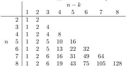
log2(ℓn,k+ 1)−log2ℓn,k!. Table 1 gives the precise values of ℓn,k for some smaller cases.
Table 1: The values ofℓn,k for some small parameters
n−k
1 2 3 4 5 6 7 8
2 1 2
3 1 2 4
4 1 2 4 8
n 5 1 2 5 10 16
6 1 2 5 13 22 32
7 1 2 6 16 31 49 64
8 1 2 6 19 43 75 105 128
Here we introduce a geometric point of view to the above problem. We introduce some notations. For a subsetI⊂[n] :={1,2, . . . , n}, putxI :=
∏
i∈Ixi, and letaIbe the element (a1, . . . , an) of{0,1}ndetermined
by ai = 1 when and only when i∈ I. We write δI :=χaI for simplicity. Let ∆
n−1
+ be the disjoint union
of an isolated point P and the standard (n−1)-simplex ∆n−1 on the vertex set [n]; we regardP as “the (−1)-dimensional face” of ∆n+−1. For each∅ ̸=I⊂[n], let⟨I⟩denote the (|I| −1)-dimensional sub-simplex of ∆n−1 spanned by I, and let ⟨I⟩o be its relative interior (note that⟨{i}⟩o=⟨{i}⟩={i} for eachi∈[n]).
On the other hand, we put⟨∅⟩=⟨∅⟩o:=P. Now for each functionf(x) =∑
I⊂[n]cIxI (cI ∈F2), we define
itsgeometric realization Gf by
Gf := ∪
I;cI=1
⟨Ic⟩o (disjoint union), (41)
where Ic denotes the complement [n]\I ofI in [n]. For each I ⊂[n], by the definition and the fact that
δI = ∑
J⊃IxJ (recall that now the values of functions are inF2),GδI is the (disjoint) union ofP and⟨J⟩
o
for all ∅ ̸=J ⊂Ic, therefore we have GδI =P∪ ⟨I
c⟩. Moreover, for any 0 ≤k≤n and I ⊂[n], we have
|I| ≥k+ 1 if and only if⟨Ic⟩is at most (n−k−2)-dimensional. This implies that a functionf ∈ Cbelongs
toCk′ if and only ifGf does not intersect with the (n−k−1)-dimensional skeleton ∆nn−k−1 of ∆
n−1 + , which
consists of the faces of ∆n+−1 of dimension up ton−k−1.
Based on the above observation, we consider the following puzzle. We imagine a situation that a lamp is associated to each face of ∆n+−1. A stateof ∆n+−1 is a collection of light/dark properties of all the lamps. Given a functionf, the correspondinginitial state If is defined in such a way that a lamp at a face is light
if and only if the relative interior of the face is contained in Gf. At any state, the player of the puzzle is
allowed to indicate a faceF of ∆n+−1(we call it “push the faceF”), then the light/dark properties of lamps atP and every sub-face ofF are flipped; such a process is regarded as amove of the puzzle. An initial state
If is said to besolved when the lamps of all faces of ∆nn−k−1are switched off by a sequence of moves started
fromIf. With this interpretation, the distanced(f,Ck′) fromf ∈ C toCk′ is the minimum of the number of
moves to solveIf, and the quantityr(C,Ck′) is the minimal necessary number of moves to solveany initial
Moreover, we also introduce a simplified puzzle on ∆n−1instead of ∆n+−1 by ignoring the isolated point P in the above puzzle. Letrn,k′ denote the minimal necessary number of moves to solve (for the simplified puzzle) any initial state. Then we haver(C,Ck′) =r′n,k+ 1, as for an initial stateI of the simplified puzzle for which solvingI requires preciselyr′n,k moves, one of the two initial states of the original puzzle obtained by adding a lamp at P which is light and dark, respectively, requires r′n,k+ 1 moves. Hence it suffices to consider the simplified puzzle on ∆n−1 for determining the quantityr(C,C′
k).
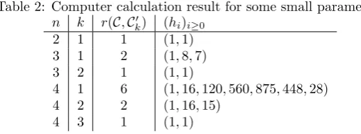
Example 1. We set n = 4 and show that r(C,C1′) = 6, or equivalently r′4,1 = 5. Note that the general bounds in Proposition 6 only guarantee that 4≤r(C,C1′)≤8 (note thatu4,1= 11>8 = 24−1). We identify
naturally each state in the puzzle on ∆n−1= ∆3with each family of non-empty subsets of [n] = [4], and we
write{i1, i2, . . . , iℓ}as i1i2· · ·iℓ for simplicity. Moreover, to express each state we omit the subsets of [4] of
size larger than 2, as the lamps at faces of dimension at least n−k−1 = 2 are not relevant to determine whether the puzzle has been solved or not. In other words, in the present situation, we can regard each state as edge and vertex coloring of the complete graphK4.
First, we show that the initial state I = {13,24} requires more than 4 moves to solve. Assume contrary that I can be solved by at most 4 moves. If the player pushes the face 1234, then a state
{1,2,3,4,12,23,34,41} is obtained. To solve the state by at most 3 remaining moves, the player has to push at least one 2-dimensional face; we may assume by symmetry that the face is 123. Then the resulting state is{4,13,34,41}; however, a case-by-case analysis shows that to solve the state by at most 2 remaining moves is impossible. Therefore the player does not push the face 1234. On the other hand, if the player pushes a 2-dimensional face, then we may assume by symmetry that the face is 123, resulting in a state
{1,2,3,12,23,24}. To solve the state by at most 3 remaining moves, the player has to push at least one more 2-dimensional face. If it is 124, then we obtain a state{3,4,23,41}, but a case-by-case analysis shows that to solve the state by at most 2 remaining moves is impossible (the case of 234 is similar by symme-try). If it is 134, then we obtain a state{2,4,12,13,14,23,24,34}, but a case-by-case analysis shows that to solve the state by at most 2 remaining moves is impossible as well. Therefore the player does not push a 2-dimensional face. This implies that the player should push 13 and 24, resulting in a state {1,2,3,4}, from which to solve the state by at most 2 remaining moves is impossible. Hence we have a contradiction, therefore the initial stateS={13,24} indeed requires more than 4 moves to solve.
Secondly, we show that any initial stateI can be solved by at most 5 moves. The player can solveI by at most 4 moves when no lamps inIat 1-dimensional faces are light, thereforeI can be solved by at most 5 moves when at most 1 lamp inIat 1-dimensional face is light. When 2 lamps inIat 1-dimensional faces are light, a case-by-case analysis shows thatIcan be solved by at most 4 moves unlessIis of the form{i1i2, i3i4}
with {i1, i2} ∩ {i3, i4} = ∅, and for any I of the latter form, I can be solved by pushing the faces 1234, i1i2i3,i1i2i4,i1, andi2. When 3 lamps inI at 1-dimensional faces are light, the problem can be reduced to
the case of 2 light lamps at 1-dimensional faces by pushing one of the 3 light lamps at 1-dimensional faces. When 4 lamps inI at 1-dimensional faces are light, the problem can be reduced to the case of 2 light lamps at 1-dimensional faces by pushing the face 1234 unless I is of the form {1,2,3,4, i1i3, i1i4, i2i3, i2i4} with
{i1, i2} ∩ {i3, i4} =∅, and for anyI of the latter form, I can be solved by pushing the facesi1i2i3,i1i2i4,
i1, andi2. When 5 lamps inI at 1-dimensional faces are light, the problem can be reduced to the case of 2 light lamps at 1-dimensional faces by pushing an appropriate 2-dimensional face. Finally, when 6 lamps inI at 1-dimensional faces are light, the problem can be reduced to the case of no light lamps at 1-dimensional faces by pushing the face 1234. Hence any initial state I can be solved by at most 5 moves, therefore we haver4′,1= 5 as desired.
From now, we investigate FDPs in the above setting by using Gr¨obner bases. Recall thatX ={0,1}n. LetR:=K[zv|v∈X] be a polynomial ring in 2n variables over a fieldK of characteristic 0. We define the
following ideal ofR:
I0:= (zv2−1|v∈X)⊂R . (42)
For eachf ∈ C, put
zf:= ∏
v∈X