PARAMETER OPTIMISATION OF RIVER WATER
QUALITY MODELS USING GENETIC
ALGORITHMS
BY
ANNE WAI MAN NG
B. Eng. Civil (Hons), Victoria University
THESIS SUBMITTED IN FULFILMENT OF THE REQUIREMENT FOR THE DEGREE OF DOCTOR OF PHILOSOPHY
SCHOOL OF THE BUILT ENVIRONMENT VICTORIA UNIVERSITY, AUSTRALIA
"^
^^'/7S/£
FTS THESIS 628.161 NG 30001007668819 Ng, Anne Wai Man
ABSTRACT
Rivers can provide valuable supply of drinking water for humans, irrigation water to
farmlands, water for hydropower and home for many aquatic ecosystems. However,
due to population increase and its adverse effects on the rivers, inappropriate fanning
activities in the river catchments, and other similar adverse activities, the water quality
in rivers has generally declined. Therefore, appropriate river water quality management
strategies aimed at controlling and improvmg water quality should be seriously
considered. At least, these strategies should not reduce further degradation of current
water quality in rivers.
To manage river water quality in the most effective and efficient way, the cause and
effect relationships of the river system must fh-st be investigated. One example of this
cause and effect relationship is the inappropriate setting of effluent hcense limits for
sewage treatment plants (STPs). Setting low effluent license lunits causes poor river
water quality with high concentration of nutrients in rivers. Water quality simulation
modelling tools are extensively used in water quality management to identify these
cause and effect relationships, and to simulate and study the effects of various 'what-if
management strategies prior to their implementation. Such a simulation model is not
available to model the Yarra River, its tributaries and associated STPs, and therefore,
the development of a water quality model for Yarra River is the focus of this thesis.
The Yarra River is one of major rivers in Melbourne in Victoria (Austraha) and is
considered as one of the most valuable assets for all Victorians. It is situated in the
eastern part of Victoria and stretches 245 km from headwaters to the mouth of estuary at
Port Phillip Bay. This river provides a major source of water supply for some 2.5
milhon Victorians, and is a major contributor to primary produce. Due to increases in
population, recent landuse developments in the catchment and inappropriate appUcation
of farming chemicals, the river water quality had degraded as indicated by the mcreases
in nutrient concentrations. This degradation of water quality in the Yarra River not only
undesirable algal blooms in Port Phillip Bay, which receives flow with high nutrients
from the Yarra River and other adjacent rivers.
Several management strategies were considered by the Environment Protection
Authority of Victoria (EPAVIC), which were used to unprove the Yarra River water
quality, in particular to reduce the nutrient level. Of these strategies, the effluent license
limits on STPs, have attracted the most attention over the past 10 years, perhaps because
the effluent discharges can easily be monitored and controlled, as they are point sources.
Furthermore, EPAVIC has planned a further stringent effluent license limit on STPs in
Year 2004. Setting of effluent license limits on STPs by EPAVIC has been solely based
on the Best Available Technology (BAT) on wastewater treatment. Although EPAVIC
has claimed that the overall water quahty has been improved with the current effluent
hcense limit upgrade, this does not guarantee further significant water quality
improvement with another stringent effluent license limit upgrade. This is because
there is a limit to the improvement of river water quality due to improvement in effluent
license limits, because the other pollutant sources become dominate then. Therefore, it
is necessary to assess the level of water quality improvement in the Yarra River with
different effluent license limits. This requires the use of a well-calibrated Yarra River
Water Quality Model (YRWQM). Due to the concern of high nutrient concentrations in
the Yarra River, nitrogen (N) and phosphorus (P) were considered in YRWQM. In
addition, dissolved oxygen (DO) was also considered, because DO is one of the major
indicators of the river health.
Development of the YRWQM considered the following steps.
• Data collection
• Selection of the appropriate software and assembly of the model
• Pre-calibration uncertainty and sensitivity analysis of model parameters
• Model calibration and verification
• Post-calibration sensitivity analysis of model parameters
The successful model development rehes primarily on the availabihty of good quality
tool for development of YRWQM. The standard river water quality software
-QUAL2E was selected for the development of YRWQM, since the available data on
STP effluent and river water quahty can be considered as steady state data, at best.
Furthermore, QUAL2E can be used to analyse 'what-if management scenarios, in
particular in relation to STP effluent license limits. An extensive data analysis was
undertaken to extract and transform valuable information to assemble YRWQM, which
included hydraulics, effluent characteristics and water quality data. The data analysis
provided the required flow events for calibration and verification of YRWQM. The
ranges for decay rates, which are responsible for degradation of river water quality,
were also determined for Yarra River through first order reaction equations for use in
the model calibration.
The model calibration is considered as one of the most important stages of the overall
model development. A prior knowledge of the effects of different model parameters to
output water quality can greatly enhance the calibration process. This can be achieved
by conducting an uncertainty and sensitivity analysis prior to model calibration, which
allows the identification of sensitive model parameters so that the modellers can
concentrate more on these parameters during calibration. The pre-calibration
uncertainty and sensitivity analysis was conducted using Monte Carlo simulation
(MCS), and the results showed that in general, all decay rates were insensitive to total
kjeldahl nitrogen (TKN), total nitrogen (TN), total phosphorus (TP) and DO
concentrations of YRWQM. This suggested that a reasonable effort can be put into
calibration of model parameters (i.e. decay rates) in this study.
The model calibration yields the set of model parameters that predicts the actual river
water quality condition. Parameter optimisation is preferred over the traditional trial
and error manual approach due to the subjectivity and time-consuming nature of the
latter approach. Furthermore, the trial and error manual approach can often miss the
'optimum' parameter set. However, the effectiveness of any optimisation method
depends on the type of search method used. Recently, an optimisation called Genetic
Algorithm (GA), which uses the concept of natural genetics as the search method, has
resource applications and therefore, was selected for this study. However, this method
has not been extensively used for parameter optimisation of river water quality models.
In general, the efficiency of GA optimisation depends on the proper selection of its
operators. These operators deal with parameter representation, population initialisation,
selection of subsequent populations, and crossover and mutation rates. Although the
importance of GA operators on model parameter optimisation has been studied in the
past, the findings were inconclusive and no guidelines were available to select
appropriate GA operators for specific applications such as optimisation of river water
quality model parameters. Therefore, a comprehensive study on the importance of GA
operators on model parameter optimisation was conducted using a hypothetical river
network model with both insensitive and sensitive parameters. The findings were then
tested with YRWQM. Based on the limited numerical experiments conducted, it was
found that the GA operators were not significant in the model with sensitive parameters
in reaching convergence to the actual parameter set. However, it was significant for the
model with insensitive parameters. Nevertheless, due to the insensitive nature of the
model, the deviation from the actual parameter set did not pose significant difference to
the actual output water quality prediction. Therefore, the use of GA in optimising
parameters of river water quality models can be done efficiently by selecting a robust
GA operator set from the literature. Although the optimised GA operator set can
guarantee the 'optimum' decay parameter set, it is necessary to consider the amount of
effort required in achieving such accuracy, which does not contribute a great difference
in the overall water quality prediction. Therefore, a GA operator set obtained from
hterature was used in the YRWQM calibration.
Eleven decay rates, which were responsible for N, P and DO were considered in
YRWQM calibration. Three low flow events were used for calibration. These low flow
events are particularly useful in calibration of decay rates, since these flow events do
not have the effect of non-point source pollution. The parameters that affect TKN and
TP (since these two are independent of each other) were first optimised, and then the
additional decay rates that affect TN were optimised keeping the previously 'optimised'
parameters of TKN constant. Finally, the additional decay rates that affect DO were
Three sets of decay rates were obtained for the three low flow events and all these
parameters were able to match water quality observations of the three low flow events at
95% significant level. Due to insignificant difference of water quality prediction
obtained from the three parameter sets, the set with the lowest cumulative absolute
relative error (CARE) was adopted as the single 'optimum' parameter set. The CARE
index was computed from the absolute difference between the observed and the
predicted water quality responses of TKN, TN, TP and DO at the six water quality
monitoring stations due to three calibration events. This single 'optimum' parameter set
was then verified using three independent low flow events which were not used in
calibration. It was found that the water quality of three events was modelled within
95% of their observed water quality.
The post-calibration sensitivity analysis is commonly used to investigate the effect of
small deviations in model parameters from the 'optimised' values on output water
quality. This post-calibration sensitivity analysis can enhance the confidence in the
'optimised' model parameters in water quality predictions and in general, in the river
water quality model itself. The commonly used 'one-at-a-time' sensitivity analysis
method was used in this study. Each of the 'optimised' decay rates was perturbed by a
certain percentage from the 'optimised' value. The results showed that even a deviation
of 50% away from the 'optimised' parameter values can predict the output water quahty
within 95% of concentration obtained from 'optimised' parameters.
The calibrated YRWQM was then used to evaluate the current point source
management strategy on STPs with different effluent license limits and to investigate
the feasibility of using a seasonal effluent discharge program to improve the water
quality in Yarra River. Comparison of the water quality improvement in both of these
cases was based on a number of effluent license limits under different river conditions.
It was found that further increase in effluent license limits on STPs does not
significantly improve Yarra River water quality, and in some cases, the wastewater
treatment based on the current hcense limits has aheady satisfied or very close to
satisfying the water quality standard. Therefore, further increases m effluent license
limits in improving Yarra River water quality is not a feasible solution. On the other
management strategy for Yarra River, due to distinct wet and dry period flows that
occur within the year. It was also found for the same effluent freatment level,
significant difference in river water quality concentration was observed for the wet and
dry period flows. Furthermore, in some instances, the water quality response from high
level of effluent treatment is very similar to the water quality response produced from a
lower level of effluent treatment under the wet conditions. Based on these findings, it
can be said that the seasonal effluent discharge program can be used as a point source
management strategy for Yarra River. This will obviously reduce the operating costs of
DECLARATION
This thesis contains no material which has been accepted for the award of any other degree or diploma in any university or institution and, to the best of the author's knowledge and belief, contains no material previously written or published by another person except where due reference is made in the text.
Anne Wai Man Ng
ACKNOWLEDGMENTS
First and foremost, I would like to sincerely thank my supervisor. Associate Professor Chris Perera, who has been a constant source of encouragement and support throughout this research project. Without his support, the completion of this thesis would not have been possible and so successful. I would also like to thank him for given me the opportunity in taking up the Yarra River Water Quality Modelling scholarship. I am also grateful to him for always been available for valuable and critical discussions and comments, in which I have gained lots of good experience contributed not only to my thesis, but also throughout my research career. His valuable time and effort in helping me getting through this thesis is very much appreciated.
I also wish to express my deepest appreciation to Dr. Andrews Takyi, who has given me the courage to take up this higher degree. I am also grateful to him for his encouragement and valuable advice.
I am thankful to The Environmental Protection Authority of Victoria, Yarra Valley Water and Melbourne Water in supplying me with data. Without their support, the project would not have been possible. Thanks also to Dr. Hao Shi and Mr. Eric Lam for their assistance in the programming. I would also like to thank the School of the Built Environment in providing me with required resources. I would also like to express my appreciation to Ms. Glenda Geyer, who was extremely helpful and supportive throughout my times at VU. Thanks also extend to officers of the postgraduate staff, who have been extremely helpful. I would also like to thank Ms Coral Ware and Ms Emily Wark of the University library, who was extremely helpful and supportive throughout my time at VU.
TABLE OF CONTENTS
ABSTRACT i DECLARATION vii
ACKNOWLEDGEMENT viii TABLE OF CONTENTS ix LIST OF FIGURES xv LIST OF TABLES xxii LIST OF ABBREVIATIONS xxv
PUBLICATIONS DURING CANDIDATURE xxvi
CHAPTER 1 INTRODUCTION
1.1 Background 1-1 1.2 River Water Quality Model Development 1-2
1.3 Significance of the Research 1-5
1.4 Aims of the Study 1-6
1.5 Outline of the Thesis 1-7
CHAPTER 2 RIVER WATER QUALITY PROCESSES AND MODELLING
2.1 Introduction 2-1 2.2 River Water Quality Processes 2-3
2.2.1 Physical processes 2-3 2.2.2 Biochemical processes 2-4 2.3 Interactions of Water Quality Constituents 2-4
2.4 River Water Quality Modelling Software 2-9 2.4.1 Catchment water quality modelling software 2-9
2.4.3 Integrated water quality software 2-17 2.4.4 Evaluation and selection of water quality software for Yarra River.... 2-18
2.5 Calibration of River Water Quality Models 2-22 2.5.1 Model parameter optimisation methods 2-23
2.5.2 Evolutionary algorithm 2-25
2.6 Genetic Algorithm 2-26 2.6.1 Genetic algorithm operators 2-27
2.6.1.1 Parameter representation 2-27 2.6.1.2 Population initialisation 2-32 2.6.1.3 Selection and sampling methods 2-33
2.6.1.4 Mutation 2-38 2.6.1.5 Crossover 2-39 2.6.1.6 Importance of GA operators 2-40
2.6.2 Application of genetic algorithm in hydrological model parameter
optimisation 2-41 2.7 Parameter Uncertainty and Sensitivity in River Water Quahty Models 2-43
2.7.1 Types of uncertainty 2-43 2.7.2 Uncertainty and sensitivity analysis methods 2-45
2.7.2.1 Local methods 2-46 2.7.2.2 Global methods 2-52 2.7.2.3 Comparison of FOEA, FORA and MCS 2-55
2.8 Summary 2-57
CHAPTER 3 DESCRIPTION OF YARRA RIVER CATCHMENT AND DATA
3.1 Introduction 3-1 3.2 Description of Yarra River Catchment 3-2
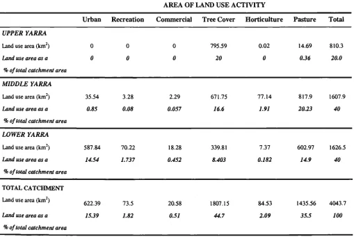
3.2.1 Landuse and catchment management 3-6 3.2.2 Water storage, diversions and streamflow measurements 3-6
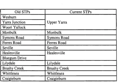
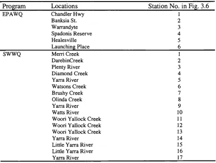
3.2.3 Sewage treatment plants (STPs) 3-9 3.2.4 Water quality sampling stations 3-12
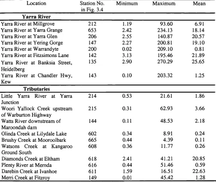
3.4 Sewage Treatment Plant Data 3-19 3.5 River Water Quality Data 3-21 3.6 Selection of Flow Events 3-22 3.7 Water Quality Data Analysis 3-23 3.8 Previous Water Quality Modelling on Yarra River Catchment 3-27
3.9 Summary 3-28
CHAPTER 4 DEVELOPMENT OF YARRA RIVER WATER QUALITY
MODEL USING QUAL2E
4.1 Introduction 4-1 4.2 QUAL2E River Water Quality Modelling Software 4-2
4.3 Discretisation ofYarra River audits Tributaries 4-8
4.4 DataLiput 4-10 4.4.1 Global group 4-10
4.4.2 Hydraulic group 4-13 4.4.2.1 Power functions for study reaches 4-14
4.4.2.2 Longitudinal dispersion 4-20
4.4.3 Reaction group 4-21 4.4.3.1 Decay rate constants 4-21
4.4.3.2 Derivation of reaeration rates 4-25
4.4.4 Incremental group 4-33 4.4.4.1 Incremental flow 4-34
4.4.4.2 Incremental concentration 4-35
4.4.5 Headwater group 4-39 4.4.5.1 Headwater flow 4-40
4.4.5.2 Headwater concentration 4-40
4.4.6 Point load group 4-44 4.4.6.1 Point load flow 4-44
4.4.6.2 Point load concentration 4-45
CHAPTER 5 PRE-CALIBRATION UNCERTAINTY AND SENSITIVITY
ANALYSIS OF MODEL PARAMETERS
5.1 Introduction 5-1 5.2 Objectives and Overall Methodology 5-3
5.3 Event and Reach Selection 5-4 5.4 Inputs Required for Monte Carlo Simulation 5-5
5.4.1 Mean values of input parameters 5-7 5.4.2 Coefficient of variation of input parameters 5-10
5.4.3 Probability density function 5-13 5.4.4 Number of simulation runs 5-13 5.5 Output Analysis in Identifying Sensitive Parameters 5-14
5.6 Analysis and Results 5-15 5.6.1 Normal and lognormal distributions 5-15
5.6.2 Identification of sensitive parameter groups 5-20 5.6.3 Sensitivity of parameters within reaction group 5-35
5.7 Summary and Conclusions 5-43
CHAPTER 6 CALIBRATION AND VERIFICATION OF YARRA RIVER
WATER QUALITY MODEL
6.1 Introduction 6-1 6.2 Flow Events Used for Calibration and Verification 6-2
6.3 Use of Genetic Algorithm for YRWQM Calibration 6-3 6.3.1 Procedures used in calibrating decay rates in YRWQM 6-4
6.4 GA Capabilities of YRWQM-GENESIS 6-7 6.5 Importance of GA Operators on Model Parameter Optimisation 6-14
6.5.1 Hypothetical river system 6-16 6.5.1.1 Development of insensitive and sensitive river models 6-16
6.5.1.2 Initial investigation of number of parameter sets and the
effect of seed 6-19 6.5.1.3 Result from hypothetical river network insensitive model 6-28
6.5.1.5 Summary of findings from hypothetical river network insensitive
and sensitive models 6-44 6.5.2 YRWQM river network 6-45 6.6 CalibrationofYarraRiver Water Quality Model 6-51
6.6.1 GA Optimisation of decay rates 6-51
6.6.1.1 TKN 6-57 6.6.1.2 TN 6-58 6.6.1.3 TP 6-59 6.6.1.4 DO 6-59 6.6.2 Selection of single optimum parameter set for YRWQM 6-61
6.7 Verification of Yarra River Water Quality Model 6-66
6.8 Post-calibration Sensitivity Analysis 6-70 6.8.1 Flow events and reaches used in sensitivity analysis 6-70
6.8.2 Input requirements and output responses 6-71
6.8.3 Results and discussion 6-72 6.9 Summary and Conclusions 6-79
CHAPTER 7 EVALUATION OF POLLUTION POINT SOURCE
MANAGEMENT POLICIES USING YRWQM
7.1 Introduction 7-1 7.2 Water Quality Management in Yarra River Catchment 7-3
7.3 Evaluation of EPAVIC Effluent License Limits 7-6
7.3.1 Low flow frequency analysis 7-7
7.3.2 Scenario development 7-9 7.3.3 Results and discussion 7-12 7.3.4 Summary of evaluation of EPAVIC effluent license limits 7-17
7.4 Seasonal Effluent Discharge Strategies 7-19 7.4.1 Seasonal flow frequency analysis 7-20 7.4.2 Generation of design conditions 7-21
7.4.3 Results and discussion 7-21 7.4.4 Summary of seasonal effluent discharge program 7-25
CHAPTER 8 SUMMARY, CONCLUSIONS AND RECOMMENDATIONS
8.1 Summary and Conclusions 8-1 8.1.1 Literature review 8-1 8.1.2 Yarra River data analysis 8-4
8.1.3 Assembly of YRWQM 8-5 8.1.4 Pre-calibration uncertainty and sensitivity analysis 8-6
8.1.5 Importance of GA operators 8-9 8.1.6 YRWQM calibration, verification and sensitivity 8-11
8.1.7 Analysis of point source management scenarios using YRWQM 8-12
8.2 Recommendations 8-13 8.2.1 Data improvement 8-13 8.2.2 GA operators 8-13
REFERENCES 9-1
APPENDICES
Appendix Al Derivation of Power Functions for Group (a) Reaches Al-l-Al-9 Appendix A2 Derivationof Power Functions for Group (b) Reaches A2-1-A2-9 Appendix B Effect of Input Parameter Coefficient of Variation
on Sensitivity of Parameter Groups B1 -B16
Appendix C Effect of Parameter Population Size On Convergence C1-C3 Appendix D Effect of Water Quality Response from Different
LIST OF FIGURES
Figure 2.1 Sources and Sink of DO 2-6
Figure 2.2 Nitrogen Cycle 2-6 Figure 2.3 Phosphorus Cycle 2-8 Figure 2.4 Summary of Public Domain Water Quality Software 2-10
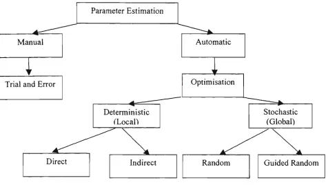
Figure 2.5 Broad Methods in Model Parameter Estimation 2-23 Figure 2.6 Conversion from Numeric Value to Binary String 2-29 Figure 2.7 Examples of Conversion from Binary Coding to Gray Coding
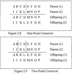
for Numeric Value 15 2-31 Figure 2.8 One-Point Crossover 2-39 Figure 2.9 Two-Point Crossover 2-39 Figure 2.10 Uniform Crossover 2-40 Figure 2.11 Summary of Uncertainty and Sensitivity Analysis Methods 2-46
Figure 3.1 Yarra River Catchment 3-3 Figure 3.2 Details of Yarra River Catchment 3-5
Figure 3.3 Water Storages in Yarra River Catchment 3-8 Figure 3.4 Gauging Stations Along Yarra River and Tributaries 3-10
Figure 3.5 Sewage Treatment Plants on Yarra River and Tributaries 3-11 Figure 3.6 EPAWQ and SWWQ Water Quality Monitoring Stations 3-13
Figure 3.7 Mean Daily Streamflow 3-17 Figure 3.8 Average Water Quality Concentrations 3-25
Figure 3.9 Average Turbidity Concentrations 3-26 Figure 4.1 QUAL2E Conceptual Representation of Stream Network 4-3
Figure 4.2 Reach Discretisation of Yarra River and Tributaries 4-9 Figure 4.3 Schematic Diagram of Discretised Yarra River and Tributaries 4-11
Figure 4.4 Cross-Section for Gauging Station 147 and Power Functions
for Reach 15 4-16 Figure 4.5 Derivationof Power Functions for Group (b) Reaches 4-19
Figure 4.6 Example of Using First Order Reaction Equation and Mass
Figure 4.8 Selection of Reaeration Method for 'Lower Range' Flows for
Main Yarra River 4-31 Figure 4.9 Selection of Reaeration Method for 'Higher Range' Flows for
Main Yarra River 4-31 Figure 4.10 Selection of Reaeration Method for 'Lower Range' Flow
for Tributaries 4-32 Figure 4.11 Selection of Reaeration Method for 'Higher Range' Flow
for Tributaries 4-32 Figure 4.12 Incremental Flow Estimation 4-34
Figure 4.13 Incremental Concentration Estimation 4-37 Figure 4.14 Estimation of Headwater Concentration 4-41 Figure 5.1 Selected River Reaches for Pre-Calibration Uncertainty
and Sensitivity Analysis 5-6 Figure 5.2 Mean Reaeration Rate Used in Monte Carlo Simulation 5-9
Figure 5.3 CDF for TN Concentration Using Normal and Lognormal PDFs
of Input Parameters ('Lower Range' Flow Event and Reach 15) 5-17 Figure 5.4 CDF for TP Concentration Using Normal and Lognormal PDFs
of Input Parameters ('Lower Range' Flow Event and for Reach 15)...5-18 Figure 5.5 CDF for DO Concentration Using Normal and Lognormal PDFs
of Input Parameters ('Lower Range' Flow Event and for Reach 15)...5-19 Figure 5.6 Relative Deviation Ratio of TBCN for 'Lower Range' Flow Event
(BaseCV) 5-21 Figure 5.7 Relative Deviation Ratio of TN for 'Lower Range' Flow Event
(BaseCV) 5-22 Figure 5.8 Relative Deviation Ratio of TP for 'Lower Range' Flow Event
(BaseCV) 5-23 Figure 5.9 Relative Deviation Ratio of DO for 'Lower Range' Flow Event
(BaseCV) 5-24 Figure 5.10 Relative Deviation Ratio of TKN for 'Higher Range' Flow Event
(BaseCV) 5-25 Figure 5.11 Relative Deviation Ratio of TN for 'Higher Range' Flow Event
Figure 5.13 Relative Deviation Ratio of DO for 'Higher Range' Flow Event
(BaseCV) 5-28 Figure 5.14 Relative Deviation Ratio for 'Lower Range' Flow Event
(BaseCV) 5-36 Figure 5.15 Relative Deviation Ratio for 'Lower Range' Flow Event
(Minimum CV) 5-37 Figure 5.16 Relative Deviation Ratio for 'Lower Range 'Flow Event
(Maximum CV) 5-38 Figure 5.17 Relative Deviation Ratio for 'Higher Range' Flow Event
(BaseCV) 5-39 Figure 5.18 Relative Deviation Ratio for 'Higher Range' Flow Event
(Minimum CV) 5-40 Figure 5.19 Relative Deviation Ratio for 'Higher Range' Flow Event
(Maximum CV) 5-41 Figure 6.1 Linkage of YRWQM and GENESIS via Input and Output Files 6-3
Figure 6.2 Systematic Process Used in Calibration of YRWQM 6-6
Figure 6.3 Schematic of YRWQM-GENESIS Run 6-8
Figure 6.4 Hypothetical River System 6-17 Figure 6.5 Parameter Range Vs Number of Parameters Taken From
Final Generation 6-21 Figure 6.6 Objective Value Vs Number of Parameter Sets Taken From Last
Generation 6-22 Figure 6.7 Effect of Seed - GA Run 1 (Statistics Based on Best 10 Values) 6-25
Figure 6.8 Effect of Seed - GA Run 2 (Statistics Based on Best 10 Values) 6-26 Figure 6.9 Effect of Seed - GA Run 3 (Statistics Based on Best 10 Values) 6-27
Figure 6.10 Convergence with Parameter Population Size of 125 6-31
Figure 6.11 Convergence with Different Mutation Rates 6-36 Figure 6.12 Convergence with Different Crossover Rate 6-38 Figure 6.13 Contour Plot of Mean Parameters with Mutation and
Crossover Rates 6-40 Figure 6.14 Contour Plot of CV with Mutation and Crossover Rates 6-41
Figure 6.15 YRWQM Water Quality Response Due to Decay Rates Obtained
Figure 6.16 YRWQM Water Quality Response Due to Decay Rates Obtained
From Different GA Operator Sets: Flow Event 18/3/92 6-50 Figure 6.17 Observed and Modelled Water Quality for Event 18/2/92
(Calibration) 6-54 Figure 6.18 Observed and Modelled Water Quality for Event 18/3/92
(Calibration) 6-55 Figure 6.19 Observed and Modelled Water Quality for Event 3/11/95
(Calibration) 6-56 Figure 6.20 Comparison of Water Quality From Different 'Optimum'
Parameter Sets for Event 18/2/92 6-62 Figure 6.21 Comparison of Water Quality From Different 'Optimum'
Parameter Sets for Event 18/3/92 6-63 Figure 6.22 Comparison of Water Quality From Different 'Optimum'
Parameter Sets for Event 3/11/95 6-64 Figure 6.23 Observed and Modelled Water Quality for Event 21/1/92
(Verification) 6-67 Figure 6.24 Observed and Modelled Water Quahty for Event 11/6/96
(Verification) 6-68 Figure 6.25 Observed and Modelled Water Quality for Event 2/4/97
(Verification) 6-69 Figure 6.26 Sensitivity of TN Decay Rates (for 'Lower Range' Flow Event) 6-73
Figure 6.27 Sensitivity of DO Decay Rates (for 'Lower Range' Flow Event) 6-74 Figure 6.28 Sensitivity of TN Decay Rates (for 'Higher Range' Flow Event) 6-75 Figure 6.29 Sensitivity of DO Decay Rates (for 'Higher Range' Flow Event) 6-76
Figure 7.1 Water Quality Comparisons for Design Case A 7-13 Figure 7.2 Water Quality Comparisons for Design Case D 7-15 Figure 7.3 Water Quality Comparisons for Event 21/1/92 with 100%
STP Discharge Volume 7-16 Figure 7.4 Water Quality Comparisons for Event 21/1/92 with 60%
STP Discharge Volume 7-18 Figure 7.5 Water Quality Comparison for Scenario Dl of Seasonal Discharge
Figure Al-1 Cross-Section for Gauging Station 103 and Power Function
for Reach 1 Al-1 Figure Al-2 Cross-Section for Gauging Station 212 and Power Function
for Reach 3 Al-2 Figure Al-3 Cross-Section for Gauging Station 602 and Power Function
for Reaches 7-9, 14 and 16 Al-3 Figure Al-4 Cross-Section for Gauging Station 653 and Power Function
for Reach 11 Al-4 Figure Al-5 Cross-Section for Gauging Station 200 and Power Function
for Reach 19 Al-5 Figure Al-6 Cross-Section for Gauging Station 142 and Power Function
for Reach 20 Al-6 Figure Al-7 Cross-Section for Gauging Station 135 and Power Function
for Reach 24 Al-7 Figure Al-8 Cross-Section for Gauging Station 143 and Power Function
for Reach 25 Al-8 Figure Al-9 Cross-Section for Gauging Station 149 and Power Function
for Reaches 21-23, 26-28 Al-9 Figure A2-1 Power Functions for Reach 2 A2-1 Figure A2-2 Power Functions for Reach 4 A2-2 Figure A2-3 Power Functions for Reach 5 A2-3 Figure A2-4 Power Functions for Reach 6 A2-4 Figure A2-5 Power Functions for Reach 10 A2-5 Figure A2-6 Power Functions for Reach 12 A2-6 Figure A2-7 Power Functions for Reach 13 A2-7 Figure A2-8 Power Functions for Reach 17 A2-8 Figure A2-9 Power Functions for Reach 18 A2-9 Figure Bl Relative Deviation Ratio of TKN for 'Lower Range' Flow Event
(Minimum CV) B-1 Figure B2 Relative Deviation Ratio of TN for 'Lower Range' Flow Event
(Minimum CV) B-2 Figure B3 Relative Deviation Ratio of TP for 'Lower Range' Flow Event
(Minimum CV) B-4 Figure B5 Relative Deviation Ratio of TKN for 'Lower Range' Flow Event
(Maximum CV) B-5 Figure B6 Relative Deviation Ratio of TN for 'Lower Range' Flow Event
(Maximum CV) B-6 Figure B7 Relative Deviation Ratio of TP for 'Lower Range' Flow Event
(Maximum CV) B-7 Figure B8 Relative Deviation Ratio of DO for 'Lower Range' Flow Event
(Maximum CV) B-8 Figure B9 Relative Deviation Ratio of TKN for 'Higher Range' Flow Event
(Minimum CV) B-9 Figure BIO Relative Deviation Ratio of TN for 'Higher Range' Flow Event
(Minimum CV) B-10 Figure Bl 1 Relative Deviation Ratio of TP for 'Higher Range' Flow Event
(Minimum CV) B-11 Figure B12 Relative Deviation Ratio of DO for 'Higher Range' Flow Event
(Minimum CV) B-12 Figure B13 Relative Deviation Ratio of TKN for 'Higher Range' Flow Event
(Maximum CV) B-13 Figure B14 Relative Deviation Ratio of TN for 'Higher Range' Flow Event
(Maximum CV) B-14 Figure B15 Relative Deviation Ratio of TP for 'Higher Range' Flow Event
(Maximum CV) B-15 Figure B16 Relative Deviation Ratio of DO for 'Higher Range' Flow Event
(Maximum CV) B-16 Figure C1 Convergence with Parameter Population Size of 250 C-1
Figure C2 Convergence with Parameter Population Size of 500 C-2 Figure C3 Convergence with Parameter Population Size of 1000 C-3
Figure Dl Water Quality Comparisons for Design Case B D-1 Figure D2 Water Quality Comparisons for Design Case C D-2 Figure D3 Water Quality Comparisons for Event 18/3/92 with 100%
Figure D5 Water Quality Comparisons for Scenario D2 of Seasonal
Discharge Program D-5
Figure D6 Water Quality Comparisons for Scenario W2 of Seasonal
Discharge Program D-6
Figure D7 Water Quality Comparisons for Scenario D3 of Seasonal
Discharge Program D-7
Figure D8 Water Quality Comparisons for Scenario W3 of Seasonal
LIST OF TABLES
Table 2.1 Evaluation Summary of QUAL2E and WASP5 Attributes 2-20
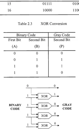
Table 2.2 Comparison Between Binary and Gray Codes 2-31
Table 2.3 XOR Conversion 2-31 Table 3.1 Land Uses in Yarra River Catchment 3-7
Table 3.2 Sewage Treatment Plant Profile 3-9 Table 3.3 Locations of Water Quality Sampling Stations 3-14
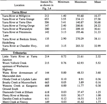
Table 3.4 Gauging Stations Used for Development of Power Functions 3-15 Table 3.5 Summary of Streamflow Range (m^/s) for Period 1992 -1997 3-16 Table 3.6 Summary of Low Flow Period Streamflow Range (m /s)
for 1992-1997 3-19 Table 3.7 Summary of High Flow Period Streamflow Range (m^/s)
for 1992-1997 3-20 Table 3.8 Summary of Mean Effluent Concentration (mg/L) ;..3-21
Table 3.9 Flow Events Selected 3-23 Table 4.1 Reach Details Modelled in YRWQM 4-12
Table 4.2 Examples for Some of the Default Entries Used in the
Global Group 4-13 Table 4.3 Temperature Correction Factors for Decay Rates 4-13
Table 4.4 Derived Power Functions 4-17 Table 4.5 Decay Rate Ranges for YRWQM Calibration 4-22
Table 4.6 Selected Reaeration Method for YRWQM 4-33 Table 4.7 Summary of Estimated Incremental Flow (m^/s) 4-36 Table 4.8 Estimated Incremental Concentrations for Event 26/7/95 4-38
Table 4.9 Summary of Statistics of Headwater Flows 4-40 Table 4.10 Summary of Estimated Range of Headwater Concentrations 4-43
Table 4.11 Categories of Point Loads Flows 4-45 Table 4.12 Summary of Point Load flows 4-46
Table 5.1 Characteristics of Flow Events Selected for Pre-Calibration
Uncertainty/Sensitivity Analysis 5-5 Table 5.2 Mean and Coefficient of Variation of Decay Rates and Reaeration
Rates Estimated from Yarra River Data and Previous Studies 5-9
Input CV Used for MCS in YRWQM 5-11 Sensitivity of Parameter Groups for Base CV 5-30
Sensitivity of Parameter Groups for Minimum CV 5-30 Sensitivity of Parameter Groups for Maximum CV 5-31 Sensitivity Ranking of Parameter Groups for Base CV 5-31 Sensitivity Ranking of Parameter Groups for Minimum CV 5-32 Sensitivity Ranking of Parameter Groups for Maximum CV 5-32 Sensitive Decay Rates Under 'Lower Range' Flow Condition 5-42 Sensitive Decay Rates Under 'Higher Range' Flow Condition 5-42
Flow Events Used for Calibration and Verification 6-3 Water Quality Decay Rates Considered in Calibration 6-5 Determination of Binary String Length for Used in
YRWQM-GENESIS 6-10 'LIT'GA Operator Set 6-15 Known Decay rates and Parameter Search Space Used in GA Runs...6-17
Runs Used to Determine the Optimum Number of Parameter Sets
Taken From the Last Generation 6-20 Table 6.7 Search Space Used for Parameter in Different GA Runs for
Hypothetical River Network 6-24 Table 6.8 Comparison on Actual and 'Optimised' Parameter Sets Obtained
from 'LIT' GA Operator Set for Hypothetical River Network
Insensitive Model 6-28 Table 6.9 Comparison of Actual and Modelled DO Concentrations (Insensitive
Model) 6-29 Table 6.10 Population Sizes Used to find the Optimum Balance 6-30
Table 6.11 Optimised GA Operator Set 6-42 Table 6.12 Comparison of the Actual and 'Optimised' Parameter Set
Obtained From Optimised GA Operator Set 6-43 Table 6.13 Comparison on Actual and 'Optimised' Parameter Set Obtained
Table 5.3 Table 5.4 Table 5.5 Table 5.6 Table 5.7 Table 5.8 Table 5.9 Table 5.10 Table 5.11 Table 6.1 Table 6.2 Table 6.3
Sensitive Model 6-43 Table 6.14 Comparison of Actual and Modelled DO Concentrations (Sensitive
Model) 6-44 Table 6.15 'LIT' and 'OPTF GA Operators Sets Used for YRWQM 6-45
Table 6.16 Progressive Reduced Search Space (day"^) for YRWQM 6-46 Table 6.17 Comparison on 'Optimised' Decay Rates with Different GA Operator
Sets 6-48 Table 6.18 'Optimised' Decay Rates From Calibration of YRWQM 6-53
Table 6.19 CARE produced by 'Optimised' Parameter Sets 6-65 Table 6.20 Flow Events Used for Post-Calibration Sensitivity Analysis 6-71
Table 6.21 'Optimised' Decay Rates of YRWQM 6-72 Table 7.1 Effluent License Limits Prior to 1997 7-5 Table 7.2 Current Effluent License Limits 7-5 Table 7.3 Design Flows Determined Using Frequency Analysis (m /s) 7-9
Table 7.4 Scenarios Considered in Evaluation of Effluent License Limits 7-10
Table 7.5 Effluent Limits for TN and TP Forms (mg/L) 7-12
LIST OF ABBREVIATIONS
The following list of abbreviations is used throughout this thesis. Other abbreviations which were only used in certain sections of the chapters are defined in that section. NH3 CBOD CBODd CBODs CV CDF DFS DO Diss-P Diss-Pben EPAVIC EPAWQ FOEA GA MCS NHjben NHs-d NO3 NO2 N02.d NOX Org-N Org-N Org-P Org-Nd Org-Ns Org-Pd Org-Ps PDF K2 RDR SOD SC STPs SWWQ TKN TN TP UYD Ammonia
Carbonaeous biochemical oxygen demand CBOD decay rate
CBOD settling rate Coefficient of variation
Cummulative distribution frequency Dights Falls
Dissolved oxygen
Dissolved phosphorus rate
Dissolved phosphorus benthos rate
Environment Protection Authority of Victoria Environment Protection Authority water quality First order error analysis
Genetic Algorithm Monte Carlo simulations NH3 benthos rate
NH3 decay rate Nitrate
Nitrite
NO2 decay rate NO2+NO3
Organic nitrogen Organic nitrogen Organic phosphorus Org-N decay rate Org-N settling rate Org-P decay rate Org-P settling rate
Probability density functions Reaeration rate
Relative deviation ratio
Sediment oxygen demand rate Sensitivity coefficient
Sewage treatment plants Stream Watch water quality
Total kjeldahl nitrogen (Org-N + NH3) Total nitrogen
PUBLICATIONS AND AWARDS DURING
CANDIDATURE
This thesis is the result of 3 years and 9 months of research work since Feb 1998 at the School of the Built Environment of Victoria University of Technology. During this period, the following research papers were published and two awards were won related to this project.
Publications
Ng. A.W.M. and Perera, B.J.C. (2001) Importance of Genetic Algorithm Operators in River Water Quality Model Parameter Optimisation. International Congress on
Modelling and Simulation (MODSIM2001), Canberra, Australia 10-13 Dec. 2001, Vol.
4, pp. 1943-1948.
Perera, B.J.C. and Ng. A.W.M. River Water Quality Modelling - Parameter Uncertainty, Sensitivity and Estimation (Invited Paper). Water Pollution 2001, Sixth
International Conference on Modelling, Measuring and Prediction of Water Pollution,
Rhodes, Greece, 17-19 Sep 2001,pp.187-196.
Ng. A.W.M. and Perera, B.J.C. Uncertainty and Sensitivity Analysis of River Water Quality Model Parameters. First International Conference on Water Resources
Management, Halkidiki, Greece, 24-26 Sep. 2001, pp. 175-184.
Ng, A.W.M. and Perera, B.J.C. (2000) Data Analysis and Preliminary Estimates of Parameters for River Water Quality Model Development, Proceedings of the 26^^
Hydrology and Water Resources Symposium, Perth, Australia, pp. 773-778.
Ng, A.W.M., Takyi, A. and Perera, B.J.C. (1999) Evaluation of Water Quahty Management Policies for the Yarra River Basin, Proceedings of the 25'^ Hydrology and
Awards
Runner-up Award for the best paper presentation at the 27''^ Hydrology and Water
Resources Symposium, Perth, Australia (2000). The paper presented was on "Data
Analysis and Preliminary Estimates of Parameters for River Water Quality Model Development".
First prize winner for the best paper presentation at the 26^^ Hydrology and Water
Resources Symposium, Brisbane, Australia (1999). The paper presented was on
CHAPTER 1
INTRODUCTION
1.1 Background
The Yarra River is one of the major rivers in Melbourne in Victoria, Australia, and is considered as one of the valuable assets for all Victorians (EPA Victoria, 1999). The Yarra River catchment has a catchment area of over 4,000 square kilometres. The forested area of the catchment provides the highest quality drinking water for over 1.5 million Victorians, while the rural area supports a thrive of agricultural industries. The urban area is becoming the focus for tourist and recreational activities.
Increase in population have resulted in extensive landuse activities in the catchment, which have been blamed for the unhealthy water quahty in the Yarra River and its tributaries. This degradation of river water quality has also caused a loss of crucial habitat for indigenous species. The Environment Protection Authority of Victoria (EPAVIC) recently identified five major environmental threats or activities in the catchment, which were responsible for the degradation of river water quahty (EPA Victoria, 1999). They are effluent discharge from sewage freatment plants (STPs), urban and rural stormwater runoff, modified flow regime, waterway erosion, and losses from sewerage system and unsewered areas. These threats, not only caused problems in the river itself, but also posed problems in Port Phillip Bay, which is also a valuable asset for all Victorians. A recent study also showed that the high level of nifrogen (N) and phosphorus (P) carried from Yarra River (and other rivers, creeks and drains) into the Bay has caused excessive algal growth (Harris et al, 1996).
progressively increased the effluent license limits of STP discharges into Yarra River
and its tributaries over the past 10 years. In Year 2004, a further upgrade of the effluent
license limits is planned so that the effluent discharge should cause no difference in the
water quality upstream and downstream of the point of discharge.
The setting of the effluent license limits on STPs by EPAVIC has been done solely on
the Best Available Technology (BAT) of wastewater treatment at the time, without
conducting detailed studies on the effect of these effluent license limits on river water
quality. As reported in EPA Victoria (1999), the upgrade of STP effluent license limits
in 1997 has improved river water quality. However, there is no guarantee that further
stringent effluent license limits can significantly improve water quality in Yarra River.
This is because there are limits to improvement of water quality through management of
STP effluent discharges. Furthermore, the other pollutant sources in the catchment
generated from river itself (i.e. resuspension of enriched nutrient sediments that were
trapped under low flows) may become dominant. However, these issues have not been
studied. Therefore, the improvement in water quality due to different effluent license
limits should be studied prior to their implementation and preferably studied in relation
to the costs (both capital and operational costs) associated with extra wastewater
treatment. The effect of the effluent license limits can be assessed through
well-calibrated river water quality models. The development of a well-well-calibrated river water
quality model for Yarra River and its tributaries including STPs is the subject of this
thesis.
1.2 River Water Quality Model Development
River water quality models are commonly used to study the responses of rivers due to
different management sfrategies, which are designed to improve water quality or at least
to manage the water quality without fiirther degradation. These models mimic the
response of the river system to various inputs (i.e. flow in the river, STPs effluent
discharges, other pollutant sources, etc.) using mathematical relationships describing
hi general, several essential stages are considered in the overall model development. They are stated in Beck (1983) and are listed below with some modifications done by the candidate.
• Data collection
• Selection of the appropriate water quality modelling software • Assembly of the model
• Calibration and verification of the model
• Uncertainty and sensitivity analysis (pre- and post-calibration) of the model parameters
Collection of accurate and reliable data is the most important stage of overall model development. If the data used in the model contain errors, then the model is not accurate. The type of available data primarily governs the selection of the water quahty modelling software. For example, if time-varying data are available, then an unsteady water quality model can be used. The assembly of the model involves data collection, analysis and then enter appropriate data into the selected computer modelling software tool. The model calibration adjusts the model parameters so that the model predictions match with the observations, and is considered also as a major step in the overall model development process. The verification process investigates the performance of the calibrated model parameters under independent events, which were not used in the calibration. The uncertainty and sensitivity analysis identifies the effect of input model parameters on the output water quality response. The model calibration and the uncertainty and sensitivity analysis of model parameters are discussed in little more detail in the next few paragraphs, since they were considered in detail in this thesis.
automatic methods have gained prominence because they can overcome some of the above shortcomings. Automatic methods can be categorised into two groups namely, deterministic and stochastic. Deterministic (or local) methods can be used when an unique solution exists for the optimum parameter set (i.e. the response surface has a single peak). On the other hand, stochastic (or global) methods are designed for situations when there are multiple peaks in the response surface from which the global optimum solution can be obtained.
There are many global automatic calibration methods available and they differ from each other in the way the searches are performed. The effectiveness of the search towards the 'optimum' parameter set depends upon the selected search algorithm. Genetic Algorithm (GA) is a global optimisation technique which has gained popularity in the recent past in many different fields, and is used in this thesis to calibrate model parameters of the Yarra River Water Quality Model (YRWQM). GA is based on the concept of natural selection and genetics (Goldberg, 1989). GA was first proposed by Holland (1975) and has since been recognised in providing a robust search in complex, noisy and discontinuous search spaces across wide disciplines (Grefenstette, 1986 and Goldberg, 1989).
In general, the efficiency of GA depends on the proper selection of GA operators, which are essentially the components that make up the overall GA process. Although there had been a number of studies conducted on the importance of the GA operators on 'optimum' model parameter set (e.g. Franchini and Galeati, 1997), the results were inconclusive. Therefore, a detailed study was conducted in this thesis on the importance of GA operators on 'optimum' model parameters of river water quality models, with particular attention given to YRWQM.
The parameter uncertainty and sensitivity analysis can be performed in two different stages in the overall model development, initially during the pre-calibration stage and later during the post-calibration stage. The pre-calibration uncertamty and sensitivity analysis can be used to identify the sensitive and insensitive model parameters, prior to model calibration. Then, it is possible to put more effort into the calibration of sensitive parameters during the calibration phase of the model development. This analysis has not been commonly considered in the past, but is a very useful analysis to be undertaken prior to calibration. On the other hand, the post-calibration sensitivity analysis is commonly used to investigate the effect of changes in the parameters deviate from the 'optimised' values, on output results. The main purpose of this sensitivity analysis is to enhance the confidence in the calibrated model so that the decision-makers can use the model confidently for assessing water quality management strategies.
1.3 Significance of the Research
Water quality of Yarra River has declined in recent years due to many factors caused by human activities. However, it has been realised that the water quality in Yarra River can be improved by good management practices. These management practices can be assessed and evaluated using water quality modelling tools. The success in the use of these modelling tools depends on how well the models are calibrated. To date, a well-calibrated water quality model has not been developed for Yarra River, which can be used to evaluate management strategies. Such a model will be developed in this study, which can be used by decision-makers to assess various water quality management scenarios. Two other significant issues were considered in this thesis, one related to model calibration and the other related to uncertainty and sensitivity analysis of model parameters.
importance of GA operators in achieving the 'optimum' parameter set will provide some guidance for modellers to use appropriate GA operators for river water quahty model parameter optimisation. Such guidelines were not available, although it was known that the efficiency of GA depends on the proper selection of GA operators.
Conducting an uncertainty and sensitivity analysis as part of the model development has been a common practice, especially at the post-calibration stage to enhance confidence in management solutions. However, conducting such analysis prior to calibration has not been commonly used. In this study, a pre-calibration uncertainty and sensitivity analysis was conducted to investigate the advantages from such analysis before calibration.
1.4 Aims of the Study
The main aim of this research project was to develop a well-calibrated water quality model for Yarra River (which is known as YRWQM in this thesis) using the GA optimisation technique. The following specific tasks were undertaken to achieve this main aim.
(i) Collect and analyse available data on the Yarra River catchment.
(ii) Select the most appropriate water quality software to develop YRWQM (iii) Assemble the YRWQM.
(iv) Select suitable low flow events for use in calibration and verification of YRWQM.
(v) Lmk YRWQM with the GA optimisation software - GENESIS through input and output files,
(vi) Conduct a pre-calibration uncertainty and sensitivity analysis of YRWQM model parameters,
(vii) Investigate the significance of GA operators in achieving the 'optimum' model parameter set of river water quality models, in particular YRWQM.
(x) Conduct a post-calibration sensitivity analysis of YRWQM model
parameters,
(xi) Investigate the effect of different management sfrategies on Yarra River
water quality.
The scope of the thesis was limited to consideration and modelling of
• Steady low flow conditions.
• Point source pollutants.
• Nonconservative water quality constituents of DO, carbonaceous
biochemical oxygen demand (CBOD), and all forms of N and P.
Steady low flow condition was considered in this study because this type of flow regime
could provide the critical water quality concentrations under various design conditions,
which provide conservative output result. Furthermore, unsteady flow and water quality
data were not available at the time of study. Due to data and time constraints, only
modelling of point source pollutants is explicitly considered in this study, although
nonpoint source was considered implicitly. Only nonconservative water quality
constituents as listed above were considered in this study because high nutrient
concentration was the major concern in the Yarra River. Modelling these
nonconservative water quality constitutes sufficiently indicate the overall river health
status of the Yarra River.
1.5 Outline of the Thesis
Chapter 2 reviewed the literature on various aspects and methods, which are required to
develop river water quality models. The type of river processes and interactions that
exist between the water quahty constituents were discussed first. Different methods that
can be used for calibration of mathematical models and uncertainty and sensitivity
analysis of model parameters were reviewed then. Comparison of various river water
quality software tools and the selection of the most appropriate water quality sofitware
Chapter 3 provided backgroimd information on the Yarra River catchment. Availability of various data for use in the model development was summarised. The selection of flow events for use in YRWQM model development was also discussed in this chapter.
Chapter 4 described the assembly of YRWQM using QUAL2E software. The estimation of the ranges for decay rates of water quality constituents for use in YRWQM calibration was discussed in this chapter, as well as the identification of
appropriate reaeration rate estimation method for Yarra River.
The pre-calibration uncertainty and sensitivity analysis of YRWQM parameters was conducted in Chapter 5.
Three main components related to parameter optimisation of YRWQM were presented in Chapter 6. First, the study of the importance of GA operators in achieving the 'optimum' parameter set was discussed. Then, the GA optimisation of YRWQM was presented together with the verification of the model. Finally, the results of the post-calibration sensitivity analysis of model parameters were presented.
The results of the investigations of point source management strategies were presented in Chapter 7. Two investigations were discussed. The first investigation dealt with different effluent license limits on STPs and their effect on Yarra River water quality. The second investigation discusses the applicability of seasonal effluent discharge programs for Yarra River catchment STPs and its effect on water quality.
CHAPTER 2
RIVER WATER QUALITY PROCESSES
AND MODELLING
2.1 Introduction
Management of river water quality has become an important issue recently, due to decline in water quality caused by many factors such as population increase and inappropriate application of farming chemicals. To be able to design and implement appropriate management sfrategies for river water quality improvement, development of river water quality models is essential. These water quality models enable the decision-makers to study the effect of various management strategies and to implement policy decisions.
A vast amount of general-purpose water quality computer software is available in the public domain, to develop catchment and river water quality models for specific river settings. These water quality modelling software can be categorised into three main groups: catchment, river and integrated. Catchment water quality soft^vare is mainly used to determine overland runoff from urban and rural areas. River water quality software, on the other hand, models river response due to the pollutants carried from overland flows and discharges from sewage treatment plants (STPs). The integrated catchment and river water quality software determines pollutant loads from the catchment and STPs within the catchment, simulates the river water quality response due to these pollutants and implements management sfrategies to improve river water quality on a basin wide scale. These software are also known as Decision Support Systems (DSSs).
manual trial and error procedures, where the predictions resulting from model parameters were compared with observations. This method is subjective, error-prone
and often by-pass the optimum parameter set (Sorooshian and Gupta, 1995). However, the automatic search methods (or optimisation methods) which have been infroduced recently for model calibration, have overcome some of these problems. In addition, the automatic search methods have demonstrated to be the most appropriate for use in water resource applications (Duan et al, 1992). Genetic algorithm (GA) is one of those parameter optimisation techniques, which has been applied recently, on a wide range of applications. GA is an optimisation technique, which utilises the concept of human genetics. In recent times, this method has also been applied to many water resource applications, and has been proven to be an efficient search technique for model parameter optimisation (Wang, 1991).
Uncertainties in model simulation have contributed to unexpectedly poor results of some stream water pollution control plans (Melching and Chang, 1996). Although there are a number of sources that contribute to model errors, the parameter estimation is the only source that can be controlled by the model user. Many methods are available which can be used to identify and quantify the effect of uncertainty and sensitivity of the input parameters to output responses.
2.2 River Water Quality Processes
River water quality depends on the assimilative capacity of the river, which is a measure of ability to digest pollutants entering the river. This assimilative capacity is controlled by 3 processes namely physical, biological and chemical (Schnoor, 1996).
2.2.1 Physical processes
The physical processes reduce organic and inorganic pollutants through dilution, sedimentation, resuspension, adsorption, volatilsation and photolysis (Chapman and Kimstach, 1992). However, these processes do not consume oxygen in reducing organic and inorganic pollutants in the river. The factors that control the amount of degradation of pollution through dilution, sedimentation, resuspension and adsorption are mainly river flow and velocity (Dojlido and Best, 1993). Dilution is a process where the water quality pollutants are reduced through the increase in 'clean' water from tributaries and other sources. Dilution is higher during high flows, although there is a possibility of high nutrient runoff being introduced during this period. Sedimentation is a process where pollutant particles such as suspended solids in the water column settles to the river bottom during low velocity periods. These settled organic matters are subject to resuspension when velocity increases, which act as another pollutant source in the water column. Adsorption is a process where the organic matters are attached to the soil particles, and eventually removed from the water column and settled in the river bottom.
2.2.2 Biochemical processes
The biological and chemical processes are often combined as biochemical processes
(Courchaine, 1968). The biochemical processes reduce or transform pollutant matter by
plants and microorganisms through consumption of oxygen (Dojlido and Best, 1993).
The degradation of organic matter through biochemical processes involves
mineralisation and microbially decaying to reduce one form of water quality constituent
to another. Mineralisation is the microbial conversion of one form of water quality
constituent to another through decomposition. Microbial decaying involves bacterial
oxidation of water quality constituents. An example of this is the nitrification, where
ammonia (NH3) oxidises to nitrite CNO2) and in turn to nifrate (NO3). Not all
biochemical processes require the presence of oxygen, for example denitrification.
Denitrification is the microbiological reduction of NO3 to NO2, which in turn can be
reduced to nifrogen gas (N2), without the presence of dissolved oxygen.
There are many factors which effect the rate of biochemical process, including
microorganism population, dissolved oxygen (DO) content, water temperature and pH
level (Bowie et al, 1985 and Dojlido and Best, 1993). The biochemical process
normally occurs in a cycle, for example nitrogen (N) and phosphorus (P). A detail
explanation of these two cycles are discussed in Section 2.3.
Both physical and biochemical processes of nonconservative water quality constituents
are considered in this thesis.
2.3 Interactions of Water Quality Constituents
The oxygen level in rivers is a crucial factor in maintaining the health of the ecosystem.
Many activities in the river catchment can cause the generation of different water
quality pollutants, which can reduce the level of DO concentration in the river. Water
quality processes, which reduce the level of oxygen level, is termed 'sinks'. On the
other hand, water quality processes, which can increase the oxygen level in rivers, is
necessary to identify these 'sources' and 'sinks' and their interactions that have effects on oxygen. However, quantifying 'sources' and 'sinks' is exfremely difficult, since there are diverse activities present in a river system (Chapra, 1998), and requires extensive data and sufficient time for analysis. In this review, major nonconservative water quality pollutants, which have effects on DO, are considered first, followed by a detailed discussion on nitrogen and phosphorus cycles.
(a) DO
Sfreeter and Phelps (1925) were the first to study the BOD-DO relationship in a river in which sinks of oxygen were caused by biodegradable waste, and the sources of oxygen were from the atmosphere. Since then, many other researchers such as Camp (1963), Dobbins (1964), and Frankel and Hansen (1968) modified and extended the Sfreeter and Phelps relationship by incorporating additional processes to enhance the accuracy of oxygen balance simulations (Gromiec et al, 1981).
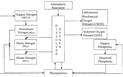
The possible nonconservative 'sources' and 'sinks' that contribute to the DO balance are shown in Figure 2.1, which has been modified from Brown and Barnwell (1987). The 'sources' and 'sinks' shovra in this figure represent primary effects on DO only, and the secondary effects are not considered in this review.
Primary effect of 'sources' is that they have direct positive (i.e. increase) influence on DO. For example, the sources of DO in Figure 2.1 include reaeration and photosynthesis of plants (e.g. phytoplankton), shown with an inward pointing arrow to DO. The secondary effects are the effects on the primary 'sources' and not directly on DO. For example, the secondary effects such as the contribution of wind, rain and hydraulic structures could effect the reaeration rate, which in turn effect the DO concenfration.
1 i 1.
Organic Nitrogen
(ORG-N)
1 '
Ammonium Nitrogen (NHJ)
^^
Nitrite Nitrogen
(NO2)
^^ Nitrate Nitrogen
(NO3)
Atmospheric Reaeration
*•
1 '
D I 0 S X S Y 0 G L E V N E D
1 J
Carbonceous Biochemical Oxygen
Demand (CBOD) Sediment Oxygen Demand (SOD)
'
Organic Phosphorus
i
Dissolved Phosphorus
4
^ —
Figure 2.1 Sources and Sinks of DO (Modified from Brown and Barnwell, 1987)
Organic nitrogen
(Org-N)
Ammonia
(NH3)
•. Miner^lisatipji. •.
. •. • Nitrifrc^tton •. •.
Nifrate
(NO3)
Plants, bacteria and aquatic
ecosystem
sediment oxygen demand (SOD) including suspended and benthic, respfration by plants and all N and P forms, as indicated with an outward pointing arrow from DO in Figure 2.1. One example of the secondary effect of 'sinks' is the influence of velocity on SOD.
Figure 2.1 also shows the interactions within N and P forms, and their interactions with phytoplankton and DO.
(b) Nifrogen cycle
The nitrogen cycle consists of microbial transformations from one form of nitrogen to another and interactions of different forms of nitrogen within the cycle. Figure 2.2 shows the nifrogen cycle. The shaded boxes shows the processes associated with various forms of N. The nifrogen forms considered in this study are organic nitrogen (Org-N), NH3, NO2, NO3. The sum of Org-N and NH3 is called total kjeldahl nifrogen (TKN), while the sum of all four forms of N is called total nitrogen (TN).
The formation of Org-N is principally through the food chain within the water body. Death of plants and aquatic organisms produce Org-N. With time, the Org-N is minerahsed to NH3. Mineralisation is the microbial fransformation from Org-N to NH3. NH3 also occurs naturally in water bodies from excretion by aquatic ecosystems, from
effluent discharges from STPs and also from runoffs from agricultural and urban lands. When the pH in water is too high, unionised NH3 can become toxic to fish (Bowie et al,
1985 and Chapra, 1998). NH3 may be adsorbed onto suspended particles (not as strongly as phosphorus) and bed sediments during low flows, and these particles would regenerate in the water column during high flows (Goering, 1972).
The reduction of NH3 is via two major processes: nitrification and uptake by aquatic plants. Nitrification involves the bacterial oxidation fransformation of NH3 to NO2, and then to NO3. The concentration of NH3 can fluctuate greatly between seasons (Bowie et
al, 1985 and Dojhdo and Best, 1993). This variation is due to greater microorganism
causmg faster fransformation with higher temperature. The product of nitrification is
NO2, but this form is unstable under aerobic conditions and hence it would rapidly
oxidised to NO3 (Bowie et al, 1985). If condition becomes anaerobic, NO3 can
partially undergo a process called denitrification and reduces back to NO2, and then
further reduced to N2, which vaporises into the atmosphere. Unfreated or inadequately
treated STP effluent can result in high levels of NH3. Runoff from excess application of
farming chemicals, death of aquatic ecosystems and debris from plants are all sources of
NO3.
(c) Phosphorus cycle
Phosphorus is another essential nutrient for growth of aquatic plants and other
microorganisms (Dojlido and Best, 1993). Phosphorus cycle is very much similar to the
nitrogen cycle, but is less complex. Phosphorus can be found in the river in two main
forms: organic and dissolved inorganic phosphorus. The source of organic phosphorus
(Org-P) is mainly from the death of plants and aquatic ecosystems. As Org-P is
generally not in a bioavailable form, it would require xmdergoing transformation to
dissolved inorganic phosphorus (Diss-P) (Reddy et al, 1999). This form is more
readily available for aquatic plant uptake (Thomann and Mueller, 1987). The rate of
breakdown of Org-P to Diss-P is depended upon the water temperature, the composition
and the bacteria population (Dojlido and Best, 1993). The phosphorus cycle is shown in
Figure 2.3. Total phosphorus (TP) is given by the sum of Org-P and Diss-P.
Organic
phosphorus
(Org-P)
Dissolved inorganic
phosphorus
(Diss-P)
Plants, bacteria and
aquatic ecosystem
Phosphorus presents in water mainly through sewage effluent discharge, soil erosion,
weathering and leaching phosphorus-bearing rocks, and runoff from agricultural and
urban areas (Bowie et al, 1985 and Dojlido and Best, 1993). Phosphorus removal from
the river is very much similar to the nitrogen removal but without the complex
nitrification and denitrification processes. Another major difference is that soil particles
adsorb sfrongly onto phosphorus. These particles then settle during low flows and
would retain in the river bed which reduce phosphorus in the water column. As Reddy
et al (1999) stated, reducing phosphorus through particle adsorption is much higher
during low summer flows than during high winter flows. Once the phosphorus settles in
the river bottom, it is subject to resuspension to release phosphorus back into the water
column during high flows. However, studies have indicated the effect of the release of
phosphorus back to the water column is insignificant over short time scales (Reddy et
al, 1999). When the oxygen content is anaerobic, the return of phosphorus back to the
water column via resuspension is three times greater as in aerobic condition. The
greater the temperature and velocity in the river water, the greater the exchange rate
between sediment and water column (Dojlido and Best, 1993).
2.4 River Water Quality Modelling Software
River water quality modelling software can be used to model the actual river system.
Many water quality modelling software tools are available and the applicability of these
software tools depends on the study objectives. Therefore, it is necessary to review
available water quality software modelling tools, so that the most appropriate software
tool can be used for the study in this thesis. This review was limited to the public
domain software. In general, the water quality modelling software can be categorised
into three broad groups, namely catchment, river and integrated software. Under these
respective groups, the available public domain software are shovm in Figure 2.4.
2.4.1 Catchment water quality modelling software
The catchment water quality modelhng software tools are used to estimate the amount
o
I
OH 00
<
• >
s
J
< O
o
w
u
•
CN
^
hJ <
D
a
w
u
•
J < Li
a
•
1—1
on
>! <
X w
•
• ^
X
o
H
S
> H VD
•
I
o
a
1-1
•s S
o O
o
.1—j OH