Line Flow Based WLS State Estimation Technique with Bad Data Measurements using PSO Algorithm

Line Flow Based WLS State Estimation

Technique with Bad Data Measurements using

PSO Algorithm

M.Kalpanadevi

, R.Neela

Assistant Professor, Dept. of Electrical Engineering, Annamalai University, Annamalai Nagar, TamilNadu, India1

Professor, Dept. of Electrical Engineering, Annamalai University, Annamalai Nagar, TamilNadu, India2

ABSTRACT: State estimation techniques are commonly used by all the utilities to make the best possible estimate of the current system state from the existing set of redundant measurements. Typically, conventional estimates produce bus voltage magnitudes and angles which need to be converted later into line loadings to conduct security analysis. Here, a novel line flow based state estimation technique that provides the output in terms of real and reactive power flows, and bus voltage magnitudes has been developed and resolved using PSO algorithm. When applied to standard test systems in the presence of various percentages of bad measurements, the suggested method has been observed to provide better results in terms of standardized error values and net computation time than conventional WLS technique.

KEYWORDS:State Estimation, Weighted Least Squares method, Line flowbased WLS, PSO and Power System.

I.INTRODUCTION

even before the state estimation algorithm estimates the system state. An identification algorithm based on the largest normalized residual considering statistical correlation among the measurements is presented in (10). As the proposed method here uses a constant Jacobian, unlike the conventional WLS estimator, the effect of bad measurements over the estimate has been significantly reduced and subsequently it doesn’t need a separate algorithm to filter out the bad measurements. Soft computing algorithms have been played a major role in solving optimization problems over the last few decades. Evolutionary programming algorithms are impressive in terms of their ability to evade local maxima and minima. Out of the many evolutionary algorithms PSO has been broadly used from the point of view of assured convergence and programming flexibility. PSO algorithm has been efficiently implemented for solving the problem of SE inspite of the apprehensions such as larger computational time etc (11-13). In this work a line flow based WLS state estimation problem has been developed and it has been solved by PSO technique in the absence as well as the presence of bad measurements for various standardized IEEE test systems.

II.CONVENTIONAL WLS STATE ESTIMATION

The aim of state estimation technique is to find out a set of state vectors that minimize the measurement residuals. The problem is basically a minimization problem and since the quantities involved are nonlinear, it is a problem of minimizing a nonlinear objective function that can be conveniently achieved using least squares technique. The measurements are expressed as a function of the state vector of the system as

(1) Here, the measurement errors which normally show normal distribution around a zero mean are assumed to be independent of each other. Each one of the measurement is assigned a acceptable weightage reflecting the accuracy and the reliability of that particular measurement whose values are decided based upon several factors such as the condition of the measuring equipment, noise of the telemetry channel etc.

The objective of WLS state estimator is to generate a suitable set of state variables in terms of bus voltage magnitudes and angles to minimize the weighted sum of the squares of the measurement errors, to achieve this the objective function is formulated as

(2)

where W is the weightage matrix, which is a diagonal matrix formed by measurement covariances when the measurements are independent of each other. The above equation is solved iteratively for estimating the state vector that minimizes J. At the end of every iteration, the state vector is updated using the correction vector as

(3)

in which obtained by solving the equation

₍₄₎

Where stands for the Jacobian and represents the gain matrix. III. PROPOSED METHOD

The proposed method tries to solve the SE problem by applying WLS technique on a line flow based model (6) which is constructed using power balance equations, line voltage equations and loop phase angle equations.

The general power balance equations for the system are written as

t T F

e T P

 

 )

( ₍₅₎

(6)

Where and are defined as bus incidence and modified bus incidence matrices in which all +1”s in are set to zeros. and represent the real and reactive power losses in the transmission lines, is an (n-1) diagonal matrix

formed by the sum of charging and compensating susceptances at each bus bar, are the real and reactive bus power injections, and are the real and reactive power flows measured at the receiving end of the transmission line. When the reactive mismatch equations are deleted at generator buses then the above equation can be rewritten as

. . (8)

in which H' is a diagonal matrix with most effective elements corresponding to load buses present in it.

The line voltage equations are composed in view of a network branch model developed without taking and considering the shunt elements including the line capacitances as,

(9)

Where k is the vector of apparent line losses, is the bus bar incidence matrix corresponding to only the PV buses,

is the vector of the square of the generator bus voltage, is the diagonal matrix of order 1 with the values equal to

the square of the tap settings, and are the positive and negative element parts of R and X are the diagonal

resistance and reactance matrices.

The loop phase angle equations are written based on the fact that the algebraic sum of phase angle drops around independent loops are zeros.

(10)

The real and reactive bus powers as a function of real line flows, reactive line flows, real line loss and reactive line loss and can be written as

(11)

(12)

Treating P, Q and as state variables the measurement set can be represented as

(13)

where . The WLS objective function is written as

(14)

As the above equation does not include line capacitances and shunt susceptances, it is inadequate to estimate the system state. However the problem is made solvable by considering the constraint equations involving branch voltage drop and phase angle variations. These equations are written as

(15)

(16)

The constrained optimization problem involving equations (14), (15) and (16) is converted into an unconstrained problem through Lagrangian multipliers as

(17)

(18)

where represent the jacobian matrices. These matrices are constant ones and the right hand side vector is split into two groups, one consisting of the bus power injections and generator bus voltages and the other consisting of nonlinear loss term and charging and compensating powers. So the vector right hand side is partially linearised. The algorithm for solving the objective function given in (18) is explained in the section below.

IV. INTRODUCTION OF PSO

PSO was first introduced in 1995 by Kennedy and Eberhart and is a heuristic optimization technique caused by swarm intelligences of animals such as bird flocking, fish schooling. A swarm of particles is the solution to the optimization problem. Each particle adjusts its position based on its own experience and the experience of its neighboring particles. The position and velocity of particle in an N – dimensional search space is expressed as

= ( ... )

= ( ... )

The best position achieved by a particle is recorded and is denoted by

= (

_,...

₎

The best particle among all the particles in the population is represented by

= ( ,... )

The updated velocity and position of each particle in _{step are calculated as follows}

_{= + (19)}

where,

_{= + (}

) + ( ) (20)

where

Iter

x

Iter

C

C

C

C



















max

1

Iter

x

Iter

C

C

C

C



















max

2

xIter

Iter

w

w

w

w























max

min

max

max

In this velocity updating process, the acceleration coefficients , and weight parameter ‘w’ are predefined and

and are uniformly generated random numbers in the range of [ 0, 1 ] and this velocity update is done until stop requirement is reached/met.

V. PSO ALGORITHM

1. Choose the population size, the number of generations, Wmin, Wmax, C1min, C1max, C2min, C2max, pbest, gbest.

2. Randomly configure all particles’ velocity and position, ensuring that they are within limits. The entities here represent the real and reactive power flows and bus voltage magnitudes.

3. Set the generation counter t=1.

5. Compare the particle's fitness function with its . If the current value is better than , then set is equal to the current value. Identify and allocate the particle to Gbest with the best success in the neighborhood so far.

6. Update velocity by using the global best and individual best of the particle.

7. Update position by using the updated velocities. Each particle will change its position. 8. If the stopping criteria is not fulfilled set t=t+1 and go to step 4.If not quit.

VI. SIMULATION AND RESULTS

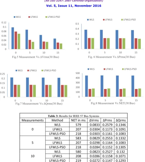
The proposed LFBSE problem has been solved using PSO technique by selecting a population size of 20 and generation size of 50 and it has been tested on standard IEEE 14, 30 and 57 bus test systems. By adding a small percentage of noise to the values obtained from the Newton Raphson load flow the measurement vector has been generated. Bus voltage magnitudes at the load buses and real and reactive power flows through the lines were taken as state variables. All the line flows, bus power injections and bus voltage magnitudes at the even numbered buses were considered in the measurement set to achieve necessary redundancy. In order to test the algorithm’s output in the presence as well as the absence of bad measurements, 5,10 and 15 numbers of bad measurements are inserted randomly in each of the measurement array. The performance of the algorithm has been confirmed by comparing the results of the proposed method against the results obtained using standard WLS state estimation and LFWLS State Estimation. With a flat start and a convergence tolerance of 0.0001, the algorithms were tested. Three performance indices are defined to validate the performance of the proposed technique. They are and

Tables 1, 2 and 3 compare the performance of the proposed method with WLS and LFWLS estimation algorithm in terms of the performance indices defined in 24, 25 and 26 and NET. The performance of the algorithm is also demonstrated in Fig 1 to 12 by bar charts.

Table 1: Results for IEEE 14 Bus Systems

Measurements Method NET in ms ΔVrms ΔPrms ΔQrms

0

WLS 197 0.148 0.1351 0.1643

LFWLS 123 0.093 0.110 0.111

LFWLS-PSO 129 0.0918 0.1097 0.1097

5

WLS 198 0.1479 0.1286 0.1631

LFWLS 123 0.0928 0.1074 0.1094

LFWLS-PSO 130 0.0913 0.1045 0.1085

10

WLS 198 0.1435 0.1277 0.1573

LFWLS 124 0.0669 0.1034 0.1083

LFWLS-PSO 130 0.0616 0.1033 0.1079

15

WLS 198 0.1421 0.1215 0.138

LFWLS 123 0.0259 0.1027 0.1078

0 0.05 0.1 0.15 0.2

0 5 10 15

Fig.3 Measurement Vs ΔQrms(14 Bus)

WLS LFWLS LFWLS-PSO

0 50 100 150 200 250

0 5 10 15

Fig.4 Measurement Vs NET (14 Bus)

WLS LFWLS LFWLS-PSO 0

0.05 0.1 0.15 0.2

0 5 10 15

Fig.1 Measurement Vs ΔVrms(14 Bus)

WLS LFWLS LFWLS-PSO

0 0.05 0.1 0.15

0 5 10 15

Fig.2 Measurement Vs ΔPrms(14 Bus)

0 0.02 0.04 0.06 0.08 0.1 0.12

0 5 10 15

Fig.5 Measurement Vs ΔVrms(30 Bus)

WLS LFWLS LFWLS-PSO

0 0.1 0.2 0.3 0.4 0.5

0 5 10 15

Fig. 6 Measurement Vs ΔPrms(30 Bus)

WLS LFWLS LFWLS-PSO

0 0.05 0.1 0.15 0.2 0.25

0 5 10 15

Fig.7 Measurement Vs ΔQrms(30 Bus)

WLS LFWLS LFWLS-PSO

0 100 200 300 400 500

0 5 10 15

Fig.8 Measurement Vs NET(30 Bus)

WLS LFWLS LFWLS-PSO

Table 3: Results for IEEE 57 Bus Systems

Measurements

Method

NET in ms

ΔVrms

ΔPrms

ΔQrms

0

WLS

579

0.0833

0.2579

0.1346

LFWLS

207

0.0304

0.1173

0.1091

LFWLS-PSO

218

0.0303

0.1161

0.1083

5

WLS

583

0.0829

0.2553

0.1332

LFWLS

207

0.0298

0.1164

0.1083

LFWLS-PSO

218

0.0284

0.1152

0.1305

10

WLS

580

0.0823

0.2527

0.132

LFWLS

208

0.0286

0.1158

0.1071

LFWLS-PSO

219

0.0272

0.1147

0.1293

15

WLS

581

0.0815

0.2502

0.1313

LFWLS

208

0.0272

0.115

0.106

VII. CONCLUSION

In this paper, a new state estimation technique that results in the formation of constant jacobian matrix has been introduced and solved for various percentages of bad measurements by PSO technique. The results indicate that when solved using PSO, the normalized value of the error between the actual values and estimated values of the state variables is considerably lower than that of the conventional WLS technique in case of proposed method. Furthermore, it can be observed that the presence of bad measurements has a significant impact on the accuracy of estimation in the conventional WLS technique whereas the proposed LFBSE technique does not. In conventional WLS estimated state variables deviates more from their true values and this deviation increases with the increase in the number of bad measurements. But this deviation is slightly less in the proposed method because that the jacobian turns out to be a constant matr ix. PSO has marginally increased the computation time and this increased computational time could be compromised against by the reduction of the normalized error values. Hence it can be concluded that the proposed PSO based LFWLS generates more accurate estimates than the conventional WLS method and it takes lesser computation time and shows less sensitivity to the presence of bad measurements, making it suitable for real time studies.

0 0.02 0.04 0.06 0.08 0.1 0.12 0.14

0 5 10 15

WLS LFWLS LFWLS-PSO

Fig.11 Measurement Vs ΔQrms(57 Bus)

0 100 200 300 400 500 600

0 5 10 15

WLS LFWLS LFWLS-PSO

Fig.12 Measurement Vs NET(57 Bus) 0

0.01 0.02 0.03 0.04 0.05 0.06 0.07 0.08 0.09

0 5 10 15

Fig.9 Measurement Vs ΔVrms(57 Bus)

WLS LFWLS LFWLS-PSO

0 0.01 0.02 0.03 0.04 0.05 0.06 0.07 0.08 0.09

0 5 10 15

Fig.10 Measurement Vs ΔPrms(57 Bus)

REFERENCES

1.Logic.N, Kyriakides.E and Heydt.G.T, 2007, “LP state estimators for power systems”, Electric Power Components and Systems, Vol. 33, No.7, pp. 669-712.

2.Pandian.A, Parthasarathy.K and Soman S.A, 1998, “A numerically stable decomposition based power system state estimation algorithm”, Electric Power and Energy Systems, Vol. 20, No.1, pp.17-23.

3.Whei-Min Lin and Jen-HaoTeng, 1998, “A new transmission fast-decoupled state estimation with equality constraints”, Electric Power and Energy Systems, Vol. 20, No.7, pp.489-493.

4.De Zhengchun, NiuZhenyong and Fang Wanliang, 2005, “Block QR decomposition based power system state estimation algorithm”, Electric Power System Research, Vol.76, pp.86-92.

5.ChakphedMadtharad, SuttichaiPremrudeepreechacharn, Neville.R Watson, 2003, “Power system state estimation using singular value decomposition”, Electric Power System Research, Vol.67, pp.99-107.

6.P.Yan, A.Sekar, 2005, “Study state analysis of power system having multiple Facts devices using line flow based equations”, IET Proceedings-Generation Transmission and Distribution, Vol.152, Issue 1, pp.31-39.

7.B.M.Zhang, S.Y.Wang and N.D.Xiang, 1992, “A linear recursive bad data identification method with real time application to power system state estimation”, IEEE Trans. on Power Systems, Vol.7, No.3, pp.1378-1385.

8.H.Salehfar, R.Zhao, 1995, “A neural network preestimation filter for bad-data detection and identification in power system state estimation”, Electric Power System Research, Vol.34, pp.127-134.

9.D.Singh, R.K.Misra, V.K.SinghR.K.Pandey, 2010, “Bad data pre-filter for state estimation”, Electric Power and Energy Systems, Vol. 32, pp.1165-1174.

10.Eduardo Caro, Antonio J.Conejo, Robert Minguez, Marija Zima and Goran Anderson, 2011, “Multiple bad data identification considering measurement dependencies”, IEEE Trans. IEEE Trans. on Power Systems, Vol.26, No.4, pp.1953-1961.

11.D.H.Tungadio, B.P.Numbi, M.W.Siti, A.A.Jimoh, 2015, “Particle swarm optimization for power system state estimation”, Neurocomputing, Vol.148, pp. 175-180.

12.Dr.M.Kalpanadevi, Dr.R.Neela, "A Novel Line Flow Based State Estimation Technique for Power Systems.” International Journal of Development Research, Volume 4, Number 4, Apr 2014, pp. 892-897. April, 2014.

13.Dr.M.Kalpanadevi, Dr.R.Neela, "Line Flow Based WLS State Estimation Technique for Power Systems with Bad Measurements.” Australian Journal of Basic and Applied Sciences, Volume 8(17), Number 1991-8178, 2014, pp. 353-359. 2014.

NOMECLATURE

LFBSE Line Flow Based State Estimation

SE State Estimation

WLS Weighted Least Squares

PM Proposed Method

PSO Particle Swarm Optimization

LFWLS Line flow based WLS

Z Measurement Vector

Initially assumed values of state vector

State vector at iteration State vector at _iteration

State correction vector after iteration

H Jacobian Matrix

h(x) Measurement function

J(x) Objective function

V Vector of measurement residues

Gain matrix

Pi Real bus power injection

Qi Reactive bus power injection

ijth element of bus incidence matrix

ijth element of modified bus incidence matrix

Pj Real power flow in jth line

Qj Reactive power flow in jth line

mj Reactive power loss in j

th line

H Diagonal matrix formed by the sum of shunt and compensating susceptances at each bus

X Diagonal matrix of line reactances

Diagonal matrix of order 1 with the values equal to the square of the tap settings

and Positive and negative element of

Lagranjian Multipliers

C Loop incidence matrix

Phase angle of the phase shifter, taken as 1 otherwise

ΔVrms,Δprms,Δqrms ΔVrms,Δprms,Δqrms –Root Mean Square values of the corresponding quantities

True values of the respective quantities on ith bus Position of individual i at iteration k

Position of individual i at iteration k + 1

Velocity of individual i at iteration k

w weight parameter

Cognitive factor

Social factor

best position of individual i until iteration k best position of group until iteration k

, random numbers between 0 and 1 wmin,wmax initial and final weights

C1min, C1max initial ad final cognitive factors C2min, C2max initial and final social factors

Itermax maximum iteration number

Iter current iteration number