www.euacademic.org DRJI Value: 5.9 (B+)
Feasibility Study of Hydrofoils Implementation in
an Emergency Speedboat
TÁSSIA CAROLINA FORASTEIRO PINTO ELIANA BRANDÃO DA SILVA DIEGO BANDEIRA DE MELO AKEL THOMAZ ARLINDO PIRES LOPES
State University of Amazonas Manaus – AM, Brazil
Abstract
The Emergency Vessels are speedboats for first aid services in several communities adjacent to Manaus, which access is restricted to the fluvial transports. Although these vessels have improved life in these communities, there is still a need for travel time reduction and making the system more efficient, as problems with service delays and fuel shortages are recurring, leaving communities without this access. Vessel fuel consumption is directly associated with the drag that is experienced when navigating at the given speed. Therefore, to make the optimization of this transports, the present project aimed to model a vessel in 1:10 scale, and to perform tests using computational and extrapolation methods. With the given results, the implementation of hydrofoils was proposed as means of optimization.
Key words: Drag; computational experiments; experimental test; hydrofoils.
1. INTRODUCTION
resources and non-compliance with projects contribute to this precariousness. The daily life of riverside communities has many restrictions induced by water dynamics, flood and ebb. Therefore, it’s necessary to implement waterway alternatives transportation in the region to improve access to difficult land areas and distant riverside communities.
According to the last demographic census of the Amazon region, this area has about 20.3 million inhabitants, of which 31.1% is riverside population. Most of them were originated from the Rubber cycle, an important commercial period in Amazonian history in the late nineteenth century, when about half a million people, mostly northeastern, moved to the northern region. Much preferred the proximity to the rivers to raise stilts. Some villages grew into municipalities. Others, smaller, were just isolated villages that still stand by the riverside to this day.
When health professionals are available, difficult access prevents them from reaching the community. Some villages are so confined in the forest that only motorized canoes can enter. It is not uncommon to find places that have never received a doctor. The Government of the State of Amazonas sought to improve access to basic health in these communities through vessels equipped with the essential equipment for emergency care and manned by two paramedics and a pilot. In 2009, 12 of these vessels were delivered with the objective of strengthening the emergency removal service of the State Department of Health in the municipalities: Alvarães, Amaturá, Anamã, Apuí, Autazes, Barcelos, Barreirinha , Beruri, Boca do Acre, Borba, Careiro Castanho, Careiro da Várzea, Codajás, Envira, Fonte Boa, Borba, Humaitá, Iranduba, Itacoatiara, Juruá, Jutaí, Manacapuru, Manicoré, Maués, Nhamundá, Novo Aripuanã, Parintins, Presidente Figueiredo, Rio Preto da Eva, Santa Izabel do Rio Negro, Santo Antônio do Içá, Tefé, Tonantins, Urucurituba.
the vessel's pilot, Erivaldo Silva, fuel consumption is very high, around 300 liters, on longer trips.
Given the problems analyzed in the field, when interviewing the crew of this vessel and collecting some of their service data, the present work aimed to make the optimization of this vessel possible. The main point analyzed was how to maintain the same power consumption for higher speeds. Fuel consumption is directly associated with the drag that the vessel experiences when sailing at a certain speed, so its study is extremely important. (Picanço, 1999).
In order to reduce travel time and fuel consumption costs, this study will show the study of the benefits of adding hydrofoils to emergency care vessels.
1.1. Drag
Initially, until 1860, the estimate of drag was made by trial and error, leading to inefficient systems and various accidents resulting from poor sizing of systems on board. In 1870, W. Froude began research for resistance testing using small-scale models and concluded that the resistance caused by wave formation varied systematically according to hull geometry and navigational speed. Following this groundbreaking study, other scholars such as Rankine, Taylor, Reynolds, and others began to investigate the effects of resistances on hull models (Molland et al., 2011).
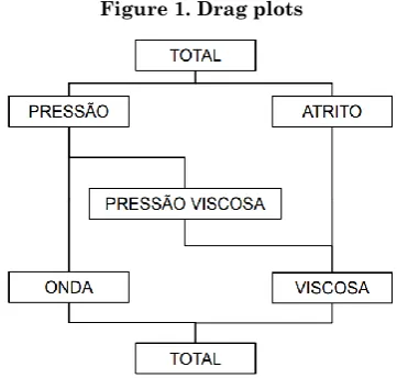
Figure 1. Drag plots
Frictional resistance is the result of the present viscosity in the flow around the hull. Pressure resistance is the result of the integral pressure field around the hull, which due to viscosity, the drag is greater ahead than astern of the boat. And the wave resistance comes from the generated waves due to hull displacement.
To obtain reliable resistance values, there are many methods, including extrapolation, statistical, and CFD methods. Those addressed in this paper include extrapolation and Savitsky's statistical method.
The extrapolation method consists of experimental tests using designed models. In which, through a scale factor, two forms of similarity are assured between ship and model, namely: geometric and dynamic. A geometric similarity is done by scale factor for the ship dimensions, and the dynamic similarity, disregarding as viscous forces, is guaranteed by the Froude number between model and ship. It’s important to note that the use of models requires the presence of test tanks to perform tests, and most tests are performed without the presence of a propulsion system. The main approaches in this area are from Froude and Hughes and the most recommended method today is ITTC 1978 (Marin, 2015).
series, however, they use some particular type of hull to measure their drag or power.
To choose the method of statistical resistance, it is important to understand the hydrodynamic elements of the vessel under study. It is possible to separate them into three simple categories according to their speed range and hydrodynamic behavior. A speed range rating is shown in Fig. 2.
Figure 2. Rating of vessels according to Froude (Molland, 2011)
While displacement vessels are supported by buoyancy forces, semi-displacement ones are supported by a mixture of buoyancy forces and dynamic lift forces, and fully planning boats are supported only by dynamic lift forces (Molland et al. , 2011).
For fully-planning vessels, characterized in the Froude range from 1.0 to 1.5, the main statistical method employed is that of Savitsky developed in 1964. The works developed by Savitsky (1964) represent the most usual method for estimating the behavior of these vessels due to its various stability and hydrodynamic parameters.
1.2. Hydrofoils
These vehicles began to be made available in 1961 in the US, following the publication of a study called “The Economic Feasibility of Passenger Hydrofoil Craft in US Domestic and Foreign Commerce”. thus beginning the same year the use of commercial hydrofoils in the US. But it was during the Cold War, especially in the 1980s, that projects advanced: Raketa was created, one of the most widely used hydrofoils in the world, Meteor, and Voskhod.
Its operation is exclusively related to the hydrodynamic shape of the profile and for the flow to remain constant, all fluid reaching the leading edge must reach the trailing edge, due to the shape of the profile, the fluid particles of the upper edge (extractor). ) develop velocities higher than those of the lower edge (intradorse). Knowing this, we see from the explicit principle in Bernoulli's equations that with a higher velocity at the upper edge the static pressure is reduced causing a pressure difference between the edges (backs?) Of the folio, resulting in an upwardly directed force.
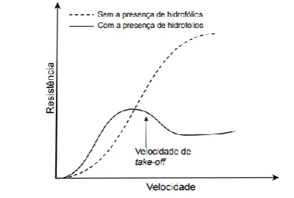
Vessels that have the application of this technology have as characteristic the curve represented in the graph of Fig.3. By comparing the drag of a vessel without hydrofoil, it has a gradual drag increasement while its speed increases. The same vessel after hydrofoil application undergoes a significant increase in resistance until the vertical force generated by the hydrofoil is able to dynamically sustain the vessel's weight (from the so-called take off speed). At this point the total drag of the vessel is gradually reduced and it can reach higher speeds.
To accomplish this project, a simplified methodology was used, which consists in the data collection of the speedboat in study, and survey of aspect ratios to characterize the vessel in its typical class. This phase was extremely important to define the study methodology of drag. From the hull lines designed in the Delftship software, a physical model was built, in a 1:10 scale. Using the model, drag tests were performed to verify whether the simplified test is able to provide consistent responses to those obtained by the Savitsky method with its own application Maxsurf Resistance software.
The test was performed with constant force values which were gradually varied so that different speeds analysis could be performed, as quoted in Artmann, 2015. The force was obtained through the free fall of a pre-determined mass, which was recorded as drag force. With values recorded from the tests and software method validation, the necessary requirements for the operation of the hydrofoil were established. In possession of the results obtained in scale tests, it was possible to verify project viability.
2. METHODOLOGY
2.1. Prototyping process
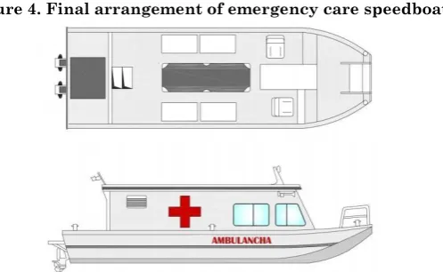
At first, a visit was made to the shipyard where the speedboat is present in Manaus, and data were collected from the second vessel shown on the Tab.1. the same.
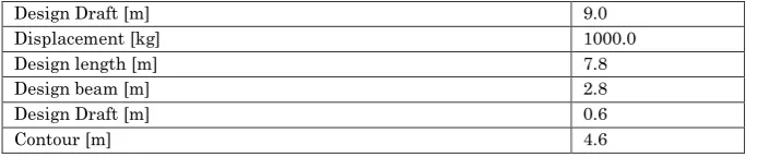
Table 1. Hull technical data from Brazilian Navy inspection
Design Draft [m] 9.0
Displacement [kg] 1000.0
Design length [m] 7.8
Design beam [m] 2.8
Design Draft [m] 0.6
Contour [m] 4.6
Figure 4. Final arrangement of emergency care speedboat
Some data collected from the speedboat outboard motor are shown below in Tab. 2.
Table 2. Outboard motor data
Tipo de Motor 24-valve, DOHC with VCT, 60 deg. V6
Vol. displacement [cm³] 3352
Diameter x stroke [mm] 94.0 x 80.5
Power [kW(Hp)] @rpm 147.1(200) @ 5500
Mass[kg] 283
Reduction 30/15
Propeller brand TL/ML
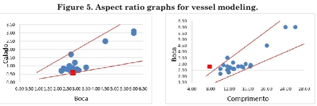
Then, the collected data were inputted in Delftship to obtain the first two-dimensional modeling of the actual speedboat.
Figure 5. Aspect ratio graphs for vessel modeling.
The reached values are within ± 6% tolerated in the design project as they will be compensated in the prototype construction by modifying the length and beam values. Thus, the values obtained in the tests that use this prototype can be compared with others within its class of boats, increasing the reliability of the results. This is a device widely used for modeling and analysis of vessels of which designs are not available.
To proceed with the construction of the model it was considered that the three conditions necessary for similarity must be followed: identically shaped parameters, performing tests on the same number of Reynolds (Re) in Eq. 1 and Froude (Fr) in Eq. 2 (Molland et al., 2011).
(1)
Where:
= Vessel speed
= Vessel design length
= Dynamic viscosity
(2)
Where:
= Gravity acceleration
similarity, incomplete similarity is used and corrections are subsequently made. Froude will be kept constant and the model speed will be calculated from Eq. 3.
(3)
Where:
= model speed
= real vessel speed
= scale factor
To make the test feasible, the chosen scale was 1:10, which is within the range of tow tank tests determined between 1:10 and 1: 100 (Chakrabarti, 1994).
Applying the scale factor to other geometric dimensions of the speedboat, beam and draft were also determined. The model total weight must be such as to generate the calculated draft. And since both (model and real) have the same block coefficient, it’s possible to obtain the model displacement through the equality shown in Eq. 4.
(4) Where:
= Volumetric displacement
= Design Beam D= Design Draft
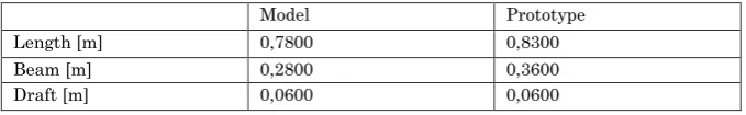
A correction was made in prototype construction to keep the results within ± 6% proposed for the project, resulting in the values presented in Table 3.
Table 3. Results comparison
Model Prototype
Length [m] 0,7800 0,8300
Beam [m] 0,2800 0,3600
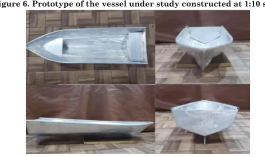
After completing aspect ratios validation within the dynamic parameters for the ITTC (2002), the vessel was built as follows in Fig. 6.
Figure 6. Prototype of the vessel under study constructed at 1:10 scale
2.2 Drag resistance analysis using Savistky's method
Through the systematic series of various authors and contributions from about four decades, Savitsky has devised a semi-empirical method considered accurate to assume the vessels dynamic lifting. There are limitations of accuracy due to the fact that calculations are based on series made with prismatic hulls, longitudinally constant, differing from most real hulls. In addition, the calculation of the longitudinal position of the pressure center is simplified, thus compromising the results of the vessel's final dynamic balance (Ribeiro, 2002).
Savitsky's method (1964) takes into account the hydrostatic forces acting on the vessel and can thus be applied to vessels operating at low speeds. Further, it proposes support and drag formulas for planing hulls, which are based on tests performed with prismatic hulls with systematic variations of trim, dead rise angle and length (Hamidon et al. 2010).
calculated automatically from any project file in the same class and then measure the required input parameters from it.
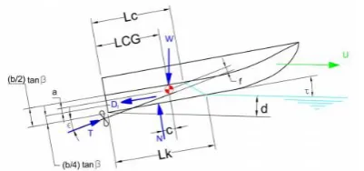
The forces acting on the vessel during the planning regime and the main geometric parameters for this method are intrinsic to the Maxsurf Resistance software and these are described by Savitsky (1964) as shown in Fig.7.
Figure 7. Planning hulls parameters (Savitsky, 1964)
Where:
= Thrust force
= Boat Weight
= Frictional Resitance
= Trim angle
= Longitudinal distance from the center of gravity measured from the stern mirror
= inclination angle of the propeller shaft, measured in relation to the keel
Resulting force from the pressure field at the bottom of the hull
Distance between and (Perpendicular measure to
Distance between and (Perpendicular measure to )
Distance between and (Perpendicular measure to N)
= Wet keel length
= wet corner length
keel draft measured at stern mirror
In a summarized way, for the method to be applied to the vessel, it’s fundamental to define its attitude, obeying the equilibrium equation
showed in Eq. 5., where the values of , , depends only on hull geometry, and weight configuration. Therefore, for the system to be
solved, the determination of , e values are required.
(5) Likewise, Savitsky's method uses several dimensionless coefficients such as frictional drag coefficient, zero deadrise angle lift coefficient, deadrise angle lift coefficient β, Reynolds number among others, which is beyond the scope of this paper.
According to Molland, Turnock and Hudson (2011), through a dimensional analysis applied to the drag forces of vessels, it’s possible
to arrive at a ratio which is a dimensionless number known as total resistance coefficient. Therefore, the vessel total drag forces can be written as shown in Eq. 6.
= (6) Where:
= fluid density
S= Wet area of the vessel
As reported by Trindade (2012), the drag force can still be defined as the force required to tow a boat at a constant speed, in calm waters. Since the effective power for this situation is obtained through Eq 7.
= (7)
Combining Eq. 6 and Eq. 7 gives Eq. 8.
= (8)
hydrofoils application on vessels, which uses the lift force generated by their shape to reduce the vessel's immersed volume, thus reducing its drag force.
2.3. Extrapolation method to drag force analysis
After the prototype geometric validation, a construct of the small-scale experiment was performed, which is an important step to provide the project continuity, because through that step the results obtained by Savitsky method will be validated. According to Artman (2015), the drag force test in test tanks consists of using the calibrated free masses, which exert constant and towing forces, thus measuring the speed that each force causes. Equipment selection should be such that they have the least impact on the test performance. To perform the tests a simplified structure will be assembled with a following list that presents the items used and their function in the procedure:
● Pool: The pool has dimensions of 8.08 meters long, 2.69 meters wide and 1.45 meters deep.
● Pole: The pole is designed exclusively for testing. It is made of steel and is 4 meters high, containing two pulleys, one at the top and one at the bottom.
● Pulleys: Pulleys were chosen that had the least possible friction and could withstand the load necessary to perform the free fall without deforming.
● Mass: To represent the mass falling from the pole, stones in bags were used, they were weighed on a commercial scale and tied to a nylon thread.
● Nylon wire: This serve to stabilize the model straight at the time of testing.
Figure 8. Free body diagram
With all the equipment prepared for the tests, it was determined the weight that would move the model. The tests were based on obtaining the time the prototype travels a distance of 2 meters, according to a mass falling from a 4-meter pole. The value of the masses used in the experiment will be based on the drag estimated through numerical analysis by Maxsurf. This obtained force was converted to a mass value measured in kilograms using Eq.9, determining for each drag a mass to be used in the experiment.
(9)
Twelve tests were performed, and the freefall was varied 3 times, thus providing 3 different points to determine the drag curve of the model. For each mass 4 measures were taken. An average of the speeds for each condition was calculated in order to decrease errors.
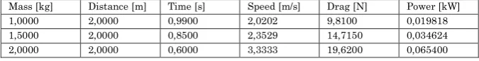
From the structure described in the free body diagram (Fig. 8), it was possible to size the experimental test as shown in Fig. 9. The average data taken from it is described in Table 4.
Figure 9. Experimental test disposition
Table 4. Data from the experiment
Mass [kg] Distance [m] Time [s] Speed [m/s] Drag [N] Power [kW]
1,0000 2,0000 0,9900 2,0202 9,8100 0,019818
1,5000 2,0000 0,8500 2,3529 14,7150 0,034624
Each drag force value was obtained according to Eq. 9, and its respective effective power from Eq. 7, shown above. It was possible, from the data collection of this prototype, to identify which drag force value the real vessel experiments during its nominal speed (≅16.67m / s) which in scale is approximately 5.26m/s. A linear regression was performed to graphically represent how the drag force behaves as a function of velocity. The equation obtained is represented in Eq. 10.
(10)
Therefore, by inputting the nominal speed of the speedboat in Eq. 10, one finds the total drag force acting on the boat, and using Eq. 7, its effective power. The data found were represented in Tab. 5.
Table 5. Scaled down vessel data (1:10)
Speed [m/s] Drag force [N] Effective Power [kW]
5,2600 33,3122 0,1752
From the obtained data it was possible to compare the drag force curves (empirical method and extrapolation method) to validate the Savitsky computational method discussed in section 2.2. The results are presented in the graph of Fig. 10.
Figure 10. Comparison of calculated drag forces.
2.3. Hydrofoil and its operation
After the method validation, we proceeded to the proposed hydrofoil design for the requirements established by this work:
• Maintain effective power at 0.1752 kW or below for a speed of 5.26 m / s (1:10 scale extrapolated speed).
• Get new speed of 9.2m/s or higher
Since the principle of using a hydrofoil is to dynamically support partially or totally the vessel's weight, a study was made on the systematic variation of the draft of the vessel under study, showing the reduction in drag force due to the reduction of the draft. This study can be seen in the graph of Fig. 11.
Figure 11. Drag analysis for each draft condition
The operation of hydrofoils is solely related to the hydrodynamic shape of the profile, knowing that for the flow to remain constant, all fluid reaching the leading edge must reach the trailing edge. Due to the shape of the profile, this will only be possible if the upper surface fluid develops a higher speed than the lower surface fluid. And through the Bernoulli equations, shown in Eq. 11, it is shown that the velocity variation between the two foil surfaces creates a pressure difference between them, thus generating the lift, as shown schematically in Fig. 12.
(11)
Where:
Figura 12. Pressure difference between the foil surface
In addition to the lift force, there are other force components that act on the foil, such as the drag force. Drag force refers to a tangential component of the viscous interaction between the fluid and the profile surface. For modeling purposes, it is assumed that the resultant of both force components acts at the center of pressure of the foil.
The equation that relates the foil lift force to the dynamic pressure is given by the lift coefficient, Cl, shown in Eq. 12., which is a function of the foil shape and the angle of attack (foil angle in relation to the flow), and determines the ability of a given profile to generate lift (Hilton, 1998).
(12)
Where:
= Lift coefficient
= Lift force
= Reference area, perpendicular to the flow
Another important equation to be defined is that which relates the drag force developed with the dynamic pressure, which is given by the drag coefficient Cd, shown in Eq. 13. By which it is possible to determine which drag is generated by the hydrofoil, and therefore what power is required to move it at a certain speed. Like the lift coefficient, the drag also depends on the shape of the profile and the angle of attack.
(13)
= Drag coefficient
= Drag force
As shown in Eq. 12, hydrofoil lift increases approximately with the square of the vessel's velocity, until the stall phenomenon occurs, which is the point at which, due to a high angle of attack, the hydrodynamic flow detaches from the profile, forming an wake with intense flow recirculation, which results in reduced lift and increased drag. According to Faltinsen (2005), the stall in hydrofoils occurs approximately at a speed of 50 knots.
The consequence of the increase in lift force is such that the submerged volume of the boat will decrease, until the dynamic equilibrium between the weight of the vessel and the lift (hydrostatic and hydrodynamic) is reached (Meyer, 1994). For these vessels to be in equilibrium, all acting forces, shown in Figure 11, must also be in equilibrium, i.e. the sum of the forces must be equal to 0, thus, by analyzing separately the x and y components, it is possible to verify the equilibrium in Eq. 14 and Eq. 15.
Figure 13. Forces acting on hydrofoil vessels.
(14)
(15) By analyzing the graph shown in Fig. 3 it is possible to verify that
develop so that the lift generated was sufficient to dynamically support the entire weight of the boat.
An important characteristic feature of takeoff speed is stability, as the lift tends to be applied on a smaller area with each draft reduction, and will be centered on the vessel's keel. In the glide condition, the lift force will be given by hydrofoils, thus having a better distribution. The use of hydrofoils reduces stability problems.
In hydrofoil arrangements the rear wing is the one that produces most of the required lift, it raises about eighty percent of the total weight of the boat, and the front wing provides most of the stability control. After the vessel's center of gravity is found, the location of the front and rear foils is determined, also based on other variables (Larsson, 2010).
Regarding arrangements, hydrofoils can be classified into two groups: surface-piercing and fully submerged as shown in Fig. 14. The main difference between these is that the former is designed to be partially out of water during the entire operation while the latter is totally submerged. Generally, submerged hydrofoils are more complex because, unlike the previous model, the structure does not self-stabilize and a system that varies the hydrofoil's angle of attack is required to control the lift force, minimizing instability problems (Aires, 2014)
Figure 14. Surface-piercing and fully submerged hydrofoils
Figure 15. Hydrofoil arrangements (DMS, 2019)
Based on the center of gravity of the speedboat under study, which is greatly influenced by the two engines, that together have a total mass of 566 kg, as mentioned in Table 2, and are at the aft of the boat, the configuration used will be Canard. This is one of the most conventional for hydrofoil vessels (Artmann, 2015).
2.4. Wing design
Having the overall hydrofoil configuration chosen, the geometric shape of each hydrofoil was designed. Initially it is necessary to choose the bidimensional foil that will be used. For this it is necessary to calculate the dimensionless hydrodynamic coefficients, which will dictate the acting forces in the hydrofoils.
To obtain these coefficients the XFOIL software was used. This simulation program enables the calculation of both viscous and non-viscous (inviscid) flows through the panel method, which consists of discretizing a geometric shape into several line segments and applying fluid dynamic singularities called vortices and sources to perform the calculation of foil features.
Several NACA series foils were analyzed, among which the best 3 were included in Tab. 6.
Table 6. Data from analyzed NACA foils
Angle of attack (α) Cl Cd Cl/Cd
NACA 63-212 4,7500° 0.6638 0.0110 57.4000
NACA 25-112 8,0000° 1.0413 0.0160 63.8800
The NACA 25-112 foil was chosen because, despite not having the highest lift coefficient, it has the highest Cl /Cd ratio, i.e. the best hydrodynamic efficiency.
Its geometric shape is shown in Fig. 16. And its main values are presented in Tab. 7.
Figure 16. NACA 25-112 foil
Table 7. Key NACA 25-112 values
Max. thickness [in chord %] 12,000% Position of max. thickness [% da corda] 29,500%
Max camber [% da corda] 2,000%
Position of max camber [% da corda] 27,200%
Stall angle 12,500°
Cl at stall angle 1,041
Cd at stall angle 0,016
In Fig. 17 it is possible to verify the relationship between variation of Cl and Cd with the variation of angle of attack α. This analysis is to verify if the angle found is close to the working limit of the foil, without the stalling phenomenon, where there is great loss of lift and significant increase of drag. It was then verified that the limit angle starts to occur at 12.5º, thus there is a good safety margin.
Figure 17. NACA 25-112 Polars.
speed (shown in Table 5) it is possible to determine from Eq. 13. what is the maximum cross-sectional area that the hydrofoil must have to not exceed such a drag, this being 0,1441 m2.
This area is about half of the projected area of the vessel's hull. With a span equal to the length of the vessel, 0.360m, the hydrofoil chord would be approximately 0.4 meters. This area will be divided between three hydrofoils, each with a chord equal to 0.12 meters each, as shown in Fig. 18.
Figure 18. 3D Wing model
3. RESULTS
Using Eq. 12, it was possible to calculate the lift generated for each speed condition. And while the force generated has not been able to dynamically support the entire weight of the vessel, it is possible to determine the volume it is lifting through the sum of forces in the vertical direction, using equation 14, which must be equal to zero. The values obtained for each situation are shown in Tab 8.
Table 8. Analytical data obtained through Maxsurf Speed [m/s] Hydrofoil displacement [ ] Hull displacement [ ] Draft [m] Drag without hydrofoil [N] Hydrofoil Drag [N] Drag with hydrofoil [N] Required power [kW]
1,6000 0,0050 0,0090 0,0373 4,4039 0,5952 4,9990 0,0080
2,4000 0,0113 0,0027 0,0114 8,4430 1,3391 9,7821 0,0235
3,2000 0,0200 0,0000 0,0000 0,0000 2,3806 2,3806 0,0076
4,0000 0,0313 0,0000 0,0000 0,0000 3,7198 3,7198 0,0149
4,8000 0,0450 0,0000 0,0000 0,0000 5,3565 5,3565 0,0257
5,6000 0,0613 0,0000 0,0000 0,0000 7,2907 7,2907 0,0408
6,4000 0,0800 0,0000 0,0000 0,0000 9,5226 9,5226 0,0609
7,2000 0,1013 0,0000 0,0000 0,0000 12,0520 12,0520 0,0868
8,0000 0,1250 0,0000 0,0000 0,0000 14,8790 14,8790 0,1190
The values obtained were shown graphically in Fig. 19 and Fig. 20. The first shows us the relationship between the drag force developed by the non-hydrofoil vessel compared to the hydrofoil vessel. In this it is possible to observe that the takeoff speed happens at approximately 3.2 m / s, from there the drag of the set reduces drastically, allowing higher speeds.
Fig. 20 further shows that the required power is still much lower than the available power, allowing the vessel to reach speeds of about 10m/s. Whereas if the speedboat could reach all its available power its speed would be limited to speeds below 6m/s.
Figure 20. Power curve with and without hydrofoils
4. CONCLUSIONS
Through this work it was possible to identify the physical viability of the implementation of hydrofoils for the emergency care vessel. With the possibility of reaching speeds close to 10m/s, which represents approximately 31m/s on the full scale boat, this means of transport could serve communities in a shorter period of time and could save more lives. It will also reduce crew discomfort as the arrangement ensures greater vertical stability.
However, some points are highlighted for this project, such as its high cost of production and maintenance, if implemented on a full scale, which is the main reason why there are not many vessels using this system.
Another approach to be analyzed in future works is the passengers' boarding and disembarking conditions, when proposing this system, as well as the influence of the waves on the effective power and speed developed.
REFERENCES
2. Artmann, J., 2015. Estudo sobre a aplicação de um hidrofólio em uma embarcação de apoio offshore: abordagem experimental simplificada. UFSC, 84 f. TCC (Graduação - Curso de Engenharia Naval).
3. Chakrabarti, S.K., 1994. Offshore Structure Modeling, Advanced series on Ocean Engineering. 9.ed. Plainfield, Illinois, USA.: Chicago Bridge & Iron Technical Service Co., World Scientific. 492p.
4. DMS., 2019. Hydrofoil control, how to stay on foil. Disponivel em: < https://dmsonline.us/hydrofoil-control-how-to-stay-on-foil/>. Acesso em: 29 de Agosto de 2019.
5. Faltinsen, Odd M. Hydrodynamics of high-speed marine vehicles. Cambridge university press, 2005.
6. Hamidon, E.; Mahamad, F. B.; As’Shaar, M. F. B., 2010.
Smk4562 [Small Craft Technology]. Universiti Teknologi Malaysia. Trabalho Acadêmico (Faculty of Mechanical Engineering)
7. Hilton, Eduardo., 1998. Aerofólios para aeronaves leves.
Disponível em:
<www.aviacaoexperimental.pro.br/aero/perfis/perfisavileve1.h tml>. Acesso em: 29 de Agosto de 2019.
8. ITTC, 2002. Internacional Towing Tank Conference. 'Testing and Extrapolation Methods, High Speed Marine Vehicles, Resistance Test', in recommended Procedures and Guidelines, p. 18.
9. Larsson, L.; Raven, H. C. “The Principles of Naval Architecture Series. New Jersey: The Society of Naval Architects, v. Ship Resistance and Flow”, 2010.
10. Marin, G., 2016. Estudo paramétrico de resistência ao avanço de uma embarcação de planeio: análise método de Savitsky. UFSC, 73 f. TCC (Graduação – Curso de Engenharia Naval) 11. Meyer, John R., 1994. Hybrid Hydrofoil Technology
Applications. Naval Engineers Journal.
13. Picanço, H.A.,1999. Resistência ao avanço: uma aplicação de dinâmica dos fluidos computacional. UFRJ, 90 f. Dissertação (Mestrado em Engenharia Oceânica).
14. Ribeiro, H. J. C., 2002. Equilíbrio Dinâmico de Cascos Planadores. UFRJ, Dissertação (Mestrado - Eng. Naval) 15. Savitsky, D. 1964. Hydrodynamic Design of Planing Hulls.
Marine Technology.