Set-point tracking of PI and PID controlled fast response flow
system
Benjamin Chinedum Oforkansi
Chemical Engineering Department, University of Lagos, Lagos, Nigeria
Abstract
The effectiveness of reference tracking of fast response flow system by conventional PI or PID controller depends on the process transfer function variables, and controller adjustable parameters. The first-order lag relationship of the flow process is obtained from the material balance, on assumption, that no reaction occurred between the input and output points. Process time constant and gain were varied from 0.005s-5s and 0.5-500 respectively while the system simple performance criteria were monitored. As expected, the controllers adjusted their time parameters by the same magnitude in which the process time constant increased, but showed insignificant change due to the increase in the process gain. The decrease in the controllers’ response time from 0.005615s to 0.00107s resulted in increased speed for the system, but at the expense of stability. Based on that, a balance between response time and robustness is required to ensure optimum set-point reference tracking and desired system stability.
Keywords: Reference, Fast Response, First-Order, Response Time, Process Gain.
1. Introduction
Various response systems occur in the process control engineering. Flow control system is a fast response system that has wide applications in the regulating of process variables [1]. For example, the adjustment of the flow rate of one or more component can be used to control the temperature of a system. [2] maintained the outlet temperature of oil close to its set-point by regulating the oil flow rate. Flow control also has wide applicability in the level control of process systems with the objective of maintaining the level around the desired set point [3]. Therefore, it is essential for control engineers to understand the dynamics of the flow systems. In most flow systems, their responses to input change depend on their capacity. Multicapacity systems are slower in response due to their inherently higher damping coefficients. On the contrary, single capacity systems respond faster to input change, and therefore require appropriate control measures that will satisfactorily keep the output signal around the
desired set point. Proportional-Integral (PI) and Proportional-Integral-Derivative (PID) controllers are used for this purpose. PI and PID controllers have been at the heart of control engineering practices for the last eight decades [4]. They have widespread acceptance in process control for variety of industries such as oil and gas, petrochemical, food and beverage, etc [5,6]. PID controllers are widely used in process industries because they are simple and easy to apply [7]. In order for the PI and PID controllers to effectively respond to the system, then the appropriate proportional, integral and derivative parameters must be selected. Therefore, proper tuning of the controller is a prime priority to the stability and performance of control systems [8]. By tuning the PID gain values, the characteristics of the closed-loop step response can be optimized to achieve a desired system output [9]. PID controllers also have additional functionalities (set-point weighting, anti-windup, etc) that allow the user to improve the performance in practical cases [10,11]. The composite proportional and integral action combined provides a balance of complexity and capability that makes it by far the most widely used algorithm in process control [12]. Specifically, they are used in flow systems [13] because they have the capacity to remove offset, and still operates within the acceptable speed. The integral component of the PI controller decreases the speed of the response but where the system response becomes sluggish; the derivative action is included to form a PID controller. The PID controller can provide the required speed and robustness through the stabilizing effect of the derivative component.
2. Methods
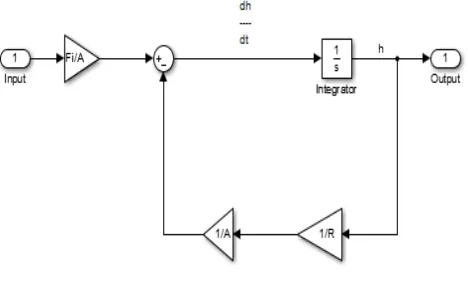
mechanism. In a feedback control system, the output variables are measured and transmitted to the controller for appropriate control actions [14]. It is assumed that the rate of flow-in is higher than the rate of flow-out; therefore, there is accumulation in the tank which will ultimately attain a steady state.
Figure 1: Flow system model
Applying the general material balance relationship gives: Accumulation=Material in - Material out +
Generation-Consumption (1) It is assumed that there is no reaction or that all the
chemical reactions have taken place prior to flow into the vessel, therefore, Generation=0 and Consumption=0.
Equation (1) becomes,
Accumulation=Material in-Material out
(2)
(3)
Where
Applying the deviation variables; and in the
equation above gives
(4)
Taking Laplace Transform of the equation
(5) At initial conditions (t=0, h=0),
Therefore (6)
Substituting AR by (time constant) and by
(steady –state gain), Equation (6) becomes:
(7)
, (8)
The transfer function is obtained:
(9)
Values of process time constant ( ) and steady-state
process gain ( ) in the range 0.005s-5s and 0.5-500
respectively were chosen, and the PI and PID controllers (Figure 2) dynamic responses were studied under the following conditions using MATLAB/Simulink software.
Figure 2: PI/PID controlled flow system
1. Increasing at constant , controller response time and transient coefficient
2. Increasing at constant and controller response time.
3. Increasing controller transient coefficient at constant , and controller response time.
3. Results and discussion
Table 1 shows the reference tracking parameters obtained
from the step plot of the feedback control of the process
given in Equation (9). The process time constant ( ) is
increased from 0.005 (at the multiples of 10) to 5 at
constant steady state gain, response time and transient coefficient. Time constant is the length of time the system
takes to reach approximately 63% of the steady state [15].
As increases from 0.005s to 0.5s, there is a
corresponding change in the dynamic characteristics of the
feedback control system. At =0.005s, the rise time of
the PI controller is 0.00405s while the settling time is 0.0148. It is clear from the Table 1 that the rise time and
settling time increase by the same geometrical ratio of 10
by which changes. The PI values of , peak
amplitude and overshoot% remain unchanged at 2.0848, 1.14 and 13.8 respectively. The only PI parameter that
decreases as increases is controller integral gain (ki)
which has the value 1251.36 at but reduces
to 1.2514 at .
Table 1: The step plot reference tracking parameters at constant
( =0.5), controller response time and transient coefficient
Characteristics PI PI PI PI
τp 0.005 0.05 0.5 5
Response time 0.005615 0.05615 0.5615 5.615
Transient
coefficent 0.6 0.6 0.6 0.6
Kp 2.0848 2.0848 2.0848 2.0848
Ki 1251.36 125.136 12.5137 1.2514
Td - - - -
Ti 0.001666 0.01666 0.1666 1.666
Rise Time 0.00405 0.0405 0.405 4.05
Settling Time 0.0148 0.148 1.48 14.8
Peak 1.14 1.14 1.14 1.14
Overshoot (%) 13.8 13.8 13.8 13.8
Characteristics PID PID PID PID
τp 0.005 0.05 0.5 5
Response time 0.005615 0.05615 0.5615 5.615
Transient
coefficient 0.6 0.6 0.6 0.6
Kp 2.8631 2.8631 2.8631 2.8331
Ki 1037.92 103.792 10.3792 1.0379
Td 2.81E-07 2.81E-06
2.81E-05
2.81E-04
Ti 0.002758 0.027582 0.2758 2.7582
Rise Time 0.00456 0.0456 0.456 4.56
Settling Time 0.0158 0.158 1.58 15.8
Peak 1.06 1.06 1.06 1.06
overshoot (%) 6.1 6.1 6.08 6.08
PID controller exhibits similar dynamic characteristics in all the parameters. Furthermore, the controller has
additional parameter, Td which increases from 2.8071E-07
to 2.8071E-04 as goes from 0.005 to 5. Comparing PI
and PID controllers parameters, it is obvious that PID has less values of peak amplitude (peak=1.06) and overshoot
(overshoot=6.1%). This means that PID controller achieves better stability because the less overshoot, the
more stable a system is [16,17].
Table 2 shows the effect of varying on the PI and PID
controllers system. It is obvious from the Table 2 that at
constant and constant controllers’ response, and
transient times, increase in has insignificant effect on
Table 2: The step plot reference tracking parameters at constant process
time constant ( =0.005), controller response time, and transient
coefficient
Characteristics PI PI PI PI
0.5 5 50 500
Response
time 0.0056 0.0056 0.0056 0.0056 Transient
coefficient 0.6 0.6 0.6 0.6 Kp 2.0848 0.2085 0.0208 0.0021 Ki 1251.36 125.136 12.5137 1.2514
Td - - - -
Ti 0.0017 0.0017 0.0017 0.0017 Rise Time 0.0041 0.0041 0.0041 0.0041 Settling Time 0.0148 0.0148 0.0148 0.0148
Peak 1.14 1.14 1.14 1.14
overshoot (%) 13.8 13.8 13.8 13.8
Characteristics PID PID PID PID
0.5 5 50 500
Response time 0.0056 0.0056 0.0056 0.0056
Transient
coefficient 0.6 0.6 0.6 0.6
Kp 2.8631 0.2863 0.0286 0.0029
Ki 1037.92 103.792 10.3792 1.0379
Td 2.81E-07 2.81E-07 2.81E-07 2.81E-07
Ti 0.0028 0.0028 0.0028 0.0028
Rise Time 0.0046 0.0046 0.0046 0.0046
Settling Time 0.0158 0.0158 0.0158 0.0158
Peak 1.06 1.06 1.06 1.06
overshoot (%) 6.08 6.08 6.08 6.08
As increases from 0.5 to 500, the PI peak amplitude
and overshoot values of 1.14 and 13.8% respectively
remain unchanged. This trend is also applicable to the PID
peak amplitude and overshoot% which remain steady at
1.06 and 6.08% respectively. All the time parameters (rise time, settling time, Td and Ti) of both controllers are not
affected by the increase in . For both the PI and PID
controllers, the controller proportional gain kp is the only
parameter that decreases as increases. The PI
proportional gain is 0.20848 at =5 but decreases to
0.0020848 at =500. In the same way, PID controller
shows a reduction of kp from 2.8631 to 0.0029 as is
adjusted from 5 to 500.
Table 3 shows the effect of increase in controller transient coefficient (robustness) on the PI and PID controllers at
constant , and controller response time.
Robustness is the ability of the system to remain
functioning under a wide range of disturbances [18].
Table 3: The step plot reference tracking parameters at constant , ,
and controller response time.
Characteristics PI PI PI PI
Transient
coefficient 0.6 0.66 0.73 0.8
Kp 0.2085 0.2441 0.2822 0.3161
Ki 125.136 116.6886 105.2241 92.1909
Td - - - -
Ti 0.0017 0.0021 0.0027 0.0034
Rise Time 0.0041 0.0042 0.0045 0.005
Settling Time 0.0148 0.0153 0.0158 0.0151
Peak 1.14 1.1 1.06 1.03
Characteristics PID PID PID PID
Transient
Coefficient 0.6 0.66 0.73 0.8
Kp 0.2863 0.2701 0.2822 0.3161
Ki 103.792 109.1556 105.2241 92.1909
Td 2.81E-07 2.81E-07 2.81E-07 2.81E-07
Ti 0.0028 0.0025 0.0027 0.0034
Rise Time 0.0046 0.0044 0.0045 0.005
Settling Time 0.0158 0.0153 0.0158 0.0151
Peak 1.06 1.08 1.06 1.03
overshoot (%) 5 5 5 5
As the robustness of the controllers increase, the time parameters (rise time, settling time and Ti) also increase as
well. The rise times of the PI controller are 0.00405s, 0.00423s and 0.00452s at 0.6, 0.66, and 0.73 set
robustness respectively. On the other hand, the PID rise time parameter indicates an oscillation as transient coefficient increases from 0.6 to 0.66. The value of the rise
time, first decreases from 0.00456 to 0.00441, then increases to 0.00496 at 0.8 transient coefficient.
Table 4 shows the effect of controller response time adjustment on the feedback control systems. At constant
, and controller robustness, decrease in controller
response time results in decrease of time parameters of the PI and PID control systems. The rise time and settling time parameters of the PI controller at 0.0056s (controller
response time) are 0.00405s and 0.0148s respectively. These values decrease to 0.000699s and 0.00457s
respectively at 0.00107s controller response time.
Table 4: The step plot reference tracking parameters at constant ,
, and controller transient coefficient
Characteristics PI PI PI PI
Response time 0.005615 0.003383 0.001859 0.00107
Transient
Coefficient 0.6 0.6 0.6 0.6
Kp 0.2085 0.412 0.8316 1.5189
Ki 125.136 277.1194 764.9022 2071.0779
Td - - - -
Ti 0.0017 0.0015 0.0011 0.0007
Rise Time 0.0041 0.0024 0.0013 0.0007
Settling Time 0.0148 0.0096 0.0056 0.0046
Peak 1.14 1.16 1.19 1.21
overshoot(%) 13.8 16.5 19.2 21.1
Characteristics PID PID PID PID
Response time 0.005615 0.003383 0.001859 0.00107
Transient
coefficient 0.6 0.6 0.6 0.6
Kp 0.2863 0.514 1.0132 1.7908
Ki 103.792 209.232 444.171 1069.777
Td 2.81E-07 1.69E-07 9.30E-08 5.35E-08
Ti 0.0028 0.0025 0.0023 0.0017
Rise Time 0.0046 0.0027 0.0015 0.0009
Settling Time 0.0158 0.011 0.0074 0.0049
Peak 1.06 1.08 1.08 1.09
Overshoot (%) 6.08 8.09 7.78 9.24
Similarly, the PID control system parameters (rise time
and settling time) exhibit the same characteristics when the response time is adjusted from 0.0056s to 0.00107s. While
the time parameters of both control systems decrease with the response time, the peak amplitude and overshoot%
controller are 1.14 and 13.8% at 0.0056s controller
response time. As the controller response time decreases to 0.00107s, the peak amplitude and overshoot increase to 1.21 and 21.1% respectively.
4. Conclusion
The set-point tracking of PI and PID-controlled fast flow
system has been simulated with MATLAB software at monitored process parameters and controllers’ dynamic
characteristics. Smaller values of used in the
simulation ensured that the system was operated in a condition similar to a real and practical fast response system. The transient coefficient is shown to be the most
significant controller dynamic characteristics, as it affected the system stability when adjusted rightward. Therefore, a
trade-off between robustness and response time is required to ensure the achievement of optimum reference tracking,
and at the same maintains desired system stability.
References
[1] A. Ganesan, R. Nhizant, K. Ganesh, R. Nithya, and H. kala , Comparison of PID Controller Tuning Techniques for a FOPDT system, IJEERT, 2 (4),(2014), 273-277
[2] M. Beschi, S. Dormido, J. Sanchez and A. Visioli, Two degree-of-freedom design for a send-on-delta sampling PI control strategy, Elsevier Control Engineering practice, 30, (2014), 55-66
[3] B. Kumar and R. Dhiman, Tuning of PID controller for liquid level tank system using intelligent techniques, IJCST, 2(4), (2011), 257-260
[4] H.B. Patel and S.N. Chaphekar, Developments in PID controllers: Literature survey, International Journal of Engineering Innovation & Research,1(5), (2012), 425-430 [5] A.S. El-Hamid, A.H. Eissa, A.M. Abouel-Fotouh and M.A. Abdel-Fatah, Comparison study of different structures of PID controllers, Research J. of Applied Sci., Engineering and Tech.,11 (6), (2015), 645-652
[6] S. Sathiyavathi and K. Poomani, Enhanced proportional integral derivative control strategy for magnetic ball levitation system, International Journal of Hybrid Information Technology, 9(16), (2016), 295-302
[7] P. Dutta, P. and A. Kumar, Comparison of PID Controller Tuning Techniques for liquid flow process control, GJAES, 2(1), (2016), 6-11
[8] P. Pal and S.K. Mandal , An evolutionary computing approach for PID optimization for automatic voltage regulator,
International Journal of Engineering Sciences & Research Technology, 5(4), (2016),113-116
[9] B. Rooholahi and P.L. Reddy, Concept and application of PID control and Implementation of continuous PID controller in Siemens PLCs, Indian Journal of Science and Technology, 8(35), (2015), 1-9
[10] M. Veronesi and A. Visioli, Automatic Feed-forward Tuning for PID control loops, European control conference, Zurich, (2013), 3919-3924
[11] R. Malhotra and R. Sodhi , Boiler flow control using PID and fuzzy logic controller, IJCSET,1(6), (2011), 315-319 [12] C. Chauhen, Tuning of IMC PID controller for optimized control, M.Sc. thesis, Control Engineering, Thapar University, Patiala, 2013
[13] M. Jaffar, G. Ravikiran and K. Sasidhar, Design of Boiler flow control using PSO technique with optimal stabilizing controller, IJIET, 6(2), (2015), 324-337
[14] D. Aditya and M.S. Kumar, Optimal stabilizing controller for boiler flow control using soft computing technique, IJERT, 3(12), (2014), 178-185
[15] A. Zielkowski, M. Baghione and D. Wootton, Determining System Time Constant through Experimental and Analytical Techniques, ASEE Zone 1 conference, (2014)
[16]N.L.S. Hashim, A. Yahya, T. Andromeda , M.R.A. Kadir, N. Mahmud, and S. Samion, Simulation of PSO-PI Controller of DC Motor in Micro-EDM system for Biomedical Application, Elsevier Procedia Engineering, 41, (2012),805-811
[17] K. Jagatheesan, B. Anand and M. Omar, Design of Proportional-Integral-Derivative controller using Ant Colony optimization technique in multi-area Automatic generation control, 7(4), (2015), 541-558