Effect Of Search And Weighing Parameter Of Optimization On Performance Of Nnmpc For Cstr Application

www.ijiset.com

Effect of search and weighing parameter of

optimization on performance of NNMPC for CSTR

application

Sanjay Baweja1 and Dr. Rajeev Gupta2

1

Research Scholar, Chemical Engg. Department, School of Engg. and Technology, Career Point University, Kota, Rajasthan, India

2

Professor, Electronics Engg. Department, Rajasthan Technical University, Kota, Rajasthan, India

Abstract

Continuous stirred-tank reactors (CSTR) are most commonly used in chemical industries, primarily in homogeneous liquid-phase flow reactions, where constant agitation is required. To get high productivity and quality from CSTR the control of various parameters is an important factor and application of neural networks for the purpose is an emerging trend. Neural Network based Model Predictive. In the present study NNMPC is implemented in Neural Network Toolbox of Matlab software that calculates the control input to optimize CSTR performance over a specified future time horizon. Two important NNMPC optimization parameters are namely weighing parameter(ρ) and search parameter(α) that needs to be tuned finely for improved performance of designed controller. Performance analysis is carried out by comparing output responses and error convergence plot for different values of ρ and α, the comparison table indicates suitable values needed for effective NNMPC design to control output concentration of CSTR.

Keywords: Continuous stirred tank reactor, Matlab, Model predictive control, Neural network, System Identification.

1. Introduction

A chemical engineer has to encounter the control problems of continuous stirring tank reactor(CSTR) to ensure successful operation. The problems in controlling cstr are too complex to be solved by the known techniques, therefore , neural networks models can provide an optimal solution due to its intelligent monitoring. Since the computation speed of computers is increasing everyday so it has several advantages over the real model or system.

The efficient H2 production and system control can be

provided by predictive control method combined with the robust BP based ANN modelling tool[1]. Neural networks can learn accurate models and give good nonlinear control when model equations are not known and also for disturbances[2,3]. The artificial neural network is the best

method to control the CSTR process and it is better than the conventional method because it has smaller value of mean square error (MSE)[4]. Concentration tracking of a CSTR can be done efficiently by using the algorithm called: Neural Network Approximate Generalized Predictive Control (NNAPC) that uses a combination of Artificial Neural Network (ANN) with Approximate Generalized Predictive Control technique[5]. CSTR modelling difficulties can be alleviated using Artificial Intelligent technique such as Neural Network[6,7]. NNPC and SVMPC gives better control performance than PID for set-point change as well as for load change[8,9]. By detecting various faults and with suitable control techniques, the accuracy of the desirable products in CSTR can be improved[10]. Model Predictive Control (MPC) is found to be very accurate and reliable in controlling the process variable. MPC has the ability to anticipate the future events and takes action accordingly[11]. Performance analysis of CSTR output response and error convergence plot indicates that the brent's line search based minimization routine gives best result as compared to other line searches and the NNMPC utilizing Brent's line search based minimization routine controls the output concentration effectively[12].

Literature review of earlier work clearly indicates that the application of NN for CSTR output control is attempted several times before, but none of the author included the effect of design parameters of NNMPC on the performance of CSTR. Thus an attempt had been made in the presented paper to analyze these effects.

design parameters for optimization process of NNMPC, section IV explains CSTR non-linear Plant Model and section V provides simulation model for tuning and testing of the designed controller. The results and discussions are given in Section VI, and section VII presents concluding remarks.

2. NN Model Predictive Control

The neural network model predictive controller uses a neural network model of a nonlinear plant to predict future plant performance[13]. The controller then calculates the control input that will optimize plant performance over a specified future time horizon. The first step in model predictive control is to determine the neural network plant model (system identification). Next, the plant model is used by the controller to predict future performance (optimization process).

2.1 System Identification

The first stage of model predictive control is to train a neural network to represent the forward dynamics of the plant. The prediction error between the plant output and the neural network output is used as the neural network training signal. The neural network plant model uses previous inputs and previous plant outputs to predict future values of the plant output. The structure of the neural network plant model consists of input layer, hidden layers and an output layer. This network can be trained offline in batch mode, using data collected from the operation of the plant. Training is done in batch mode using fast algorithms that uses one of the three standard numerical optimization techniques i.e. Conjugate gradient; Quasi-Newton and Levenberg-Marquardt (trainlm).

2.2 Predictive Control

The model predictive control method is based on the receding horizon technique [14]. The neural network model predicts the plant response over a specified time horizon. The predictions are used by a numerical optimization program to determine the control signal that minimizes the following performance criterion over the specified horizon

(1)

where N1, N2, and Nu define the horizons over which the tracking error and the control increments are evaluated.

The u′ variable is the tentative control signal, yr is the desired response, and ym is the network model response. The ρ value determines the contribution that the sum of the squares of the control increments has on the performance index.

Fig.1 illustrates the block diagram for model predictive control process. The controller consists of the neural network plant model and the optimization block. The optimization block determines the values of u′ that

minimize J, and then the optimal u is input to the plant. The controller block is implemented in Matlab simulink, as described in the section V.

Fig.1 Block diagram of model predictive control process

3. Optimization of Neural Network Model

In optimization, the line search strategy is one of two basic iterative approaches to find a local minimum x* of an objective function f : Rn → {R}. The other approach is trust region.

A line search algorithm seeks the minimum of a defined nonlinear function by selecting a reasonable direction vector that, when computed iteratively with a reasonable search parameter, will provide a function value closer to the absolute minimum of the function. Varying these will change the "tightness" of the optimization. For example, given the function f(x), an initial xk is chosen. To

find a lower value of f(x), the value of xk+1 is increased by

the following iteration scheme: xk+1=xk+αkpk,

in which αk is a positive scalar known as the search

parameter or step length and pk defines the step direction.

y

u u '

y ym

Plant Neural Network

Model Optimization

www.ijiset.com

3.1 Search parameter (step length)

Choosing an appropriate search parameter has a large impact on the robustness of a line search method. To select the ideal search parameter, the following function could be minimized:

φ(α) = f(xk + αpk), α>0,

but this is not used in practical settings generally. This may give the most accurate minimum, but it would be very computationally expensive if the function φ has multiple local minima or stationary points[15].

A common and practical method for finding a suitable step length that is not too near to the global minimum of the φ function is to require that the search parameter of αk reduces the value of the target function, or that f(xk +

αpk < f(xk).

This method does not ensure a convergence to the function's minimum, and so two conditions are employed to require a significant decrease condition during every iteration.

4. Plant Model

A standard catalytic Continuous Stirred Tank Reactor (CSTR) model is used in the present study. The diagram of the process is shown in the Fig. 2.

Fig. 2 Plant Model[13]

The dynamic model of the system is :

(2)

(3)

where h(t) is the liquid level, Cb(t) is the product concentration at the output of the process, w1(t) is the flow

rate of the concentrated feed Cb1, and w2(t) is the flow rate

of the diluted feed Cb2. The input concentrations are set to Cb1 = 24.9 and Cb2 = 0.1. The constants associated with

the rate of consumption are k1 = 1 and k2 = 1.

The objective of the controller is to maintain the product concentration by adjusting the flow w1(t). To

simplify the example, set w2(t) = 0.1. The level of the tank h(t) is not controlled for this experiment[13].

5. Simulation Model

A diagram of the simulation process is shown in Fig.3, it includes a catalytic Continuous Stirred Tank Reactor (CSTR) whose output concentration is controlled via NNPC, input to the controller is set to a random reference signal.

Fig. 3 Block diagram of simulation model

Plant identification is done to develop the neural network plant model to predict future plant outputs. The optimization algorithm uses these predictions to determine the control inputs that optimize future performance. The plant model neural network has seven hidden layer, the number of delayed inputs-2 nos. and delayed outputs-2 nos., and the training function is trainlm to train the neural network plant model. Then training data is generated which is further used to train the network(plant model) according to the training algorithm. Simulation is performed after loading the trained neural network plant model into the NN Predictive Controller block.

The NN Predictive Controller is designed by setting controller horizons N2 and Nu(N1 is fixed at 1.), weighing

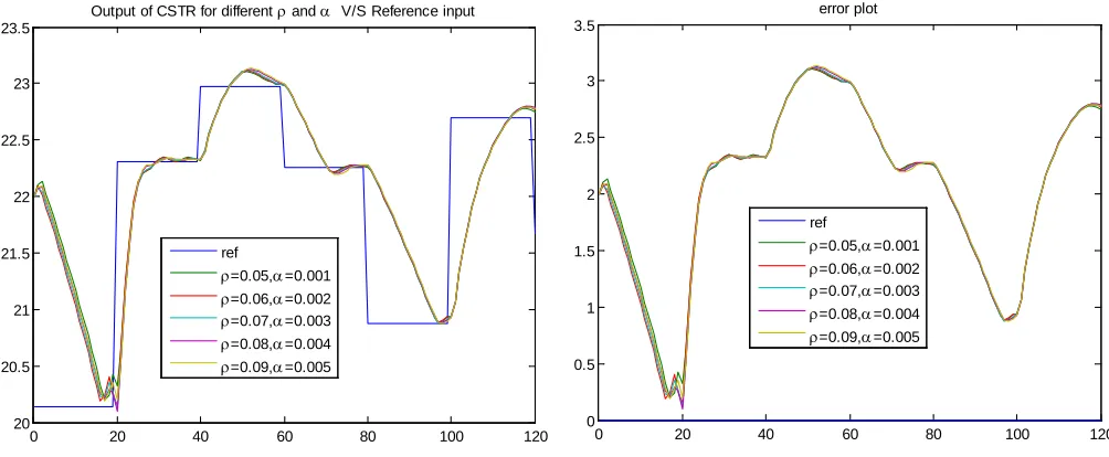
parameter ρ and search parameter α to control the optimization. It determines how much reduction in performance is required for a successful optimization step. Brent's line search based minimization routine[12] is used by the optimization algorithm, and 2 iterations of the optimization algorithm are performed at each sample time. As the simulation runs, the plant output for different ρ and α and the random reference signal are displayed, as in the Fig.4. Also the error convergence plot is shown in Fig.5 that compares the reference signal with 5 outputs having different values of ρ and α to optimize the neural network predictive controller.

Random Reference

NNMPC Plant

(CSTR)

0 20 40 60 80 100 120 20

20.5 21 21.5 22 22.5 23 23.5

Output of CSTR for different ρ and α V/S Reference input

ref

ρ=0.05,α=0.001 ρ=0.06,α=0.002 ρ=0.07,α=0.003 ρ=0.08,α=0.004 ρ=0.09,α=0.005

Fig.4 Output response of CSTR for different values of ρ and α v/s ref. signal

0 20 40 60 80 100 120

0 0.5 1 1.5 2 2.5 3 3.5

error plot

ref

ρ=0.05,α=0.001 ρ=0.06,α=0.002 ρ=0.07,α=0.003 ρ=0.08,α=0.004 ρ=0.09,α=0.005

Fig.5 Error convergence plot for five different combinations of ρ and α.

Table 1 Comparison of statistical characteristics of five different combinations of ρ and α.

Statistics Ref signal ρ =0.05

α = 0.001

ρ =0.06 α = 0.002

ρ=0.07 α=0.003

ρ =0.08 α=0.004

ρ =0.09 α=0.005

Min 20.137 20.198 20.151 20.113 20.099 20.192

Max 22.975 23.104 23.113 23.118 23.125 23.132

Mean 21.874 22.058 22.042 22.043 22.05 22.054

Median 22.255 22.261 22.264 22.257 22.271 22.267

Mode 20.137 20.198 20.151 20.113 20.099 20.192

Std 1.021 0.75155 0.77596 0.77596 0.77252 0.76752

range 2.8385 2.9059 2.9617 3.005 3.0253 2.9402

6. Results and Discussions

Fig.4 shows the output concentration response of CSTR corresponding to different values of ρ and α used for optimization of NNMPC. Fig.5 indicates the error convergence in the five conditions, using data statistics tool in Matlab a comparison is obtained for the five conditions. Table 1 gives the comparison of statistical parameters for varying parameters and shows that ρ = 0.05 and α = 0.001 error converges more effectively and has minimum magnitude of range and standard deviation, hence it is best suited for the particular application.

7. Conclusions

www.ijiset.com

References

[1] Nikhil, B.Özkaya, A.Visa, C.Y. Lin, J. A. Puhakka, and O.Yli-Harja, "An Artificial Neural Network Based Model for Predicting H2 Production Rates in a Sucrose-Based Bioreactor System", International Journal of Chemical, Molecular, Nuclear, Materials and Metallurgical Engineering Vol.2, No.1, 2008, pp 1-6.

[2] R.S.M. Malar and T. Thyagarajan, "Artificial Neural Networks Based Modeling and Control of Continuous Stirred Tank Reactor", American J. of Engineering and Applied Sciences, Vol.2. No.1, 2009, pp. 229-235.

[3] B.Z. Nezhad and A. Aminian, "Application of the Neural Network-based Model Predictive Controllers in Nonlinear Industrial Systems: Case Study", Journal of the University of Chemical Technology and Metallurgy, Vol.46, No.1, 2011, pp. 67-74.

[4] K.M. Putrus, "Implementation of Neural Control for Continuous Stirred Tank Reactor (CSTR)", Al-Khwarizmi Engineering Journal, Vol.7, No.1, 2011, pp. 39-55.

[5] H.E. Kalhoodashti, "Concentration Control of CSTR using NNAPC", International Journal of Computer Applications, Vol. 26, No.6, 2011, pp. 34-38.

[6] P. Shrivastava, "Modeling and Control of CSTR using Model based Neural Network Predictive Control", International Journal of Computer Science and Information Security, Vol.10, No.7, 2012, pp. 38-43.

[7] A. Kumar, M. Bajaj and P.N. Verma, "Implementation of Neural Model Predictive Control in Continuous Stirred Tank Reactor System", International Journal of Scientific & Engineering Research, Vol.4, No.6, 2013, pp. 1989-1996. [8] N. Sharma and K. Singh, "Neural network and support vector

machine predictive control of tert-amyl methyl ether reactive distillation column", Systems Science & Control Engineering: An Open Access Journal, Vo.2, No.1, 2014, pp. 512–526. [9] P. Ghutke and A.B. Patil, "Performanance analysis of Neural

network based NARMA control of CSTR", International Journal for Innovative Research in Science & Technology, Vol.1, No.8, 2015, pp. 216-222.

[10] R. Gowthami and Dr. S. Vijayachitra, "Fault Detection and Diagnosis in Continuous Stirred Tank Reactor", International Journal of Technical Research and Applications, Vol.3, No.2, 2015, pp. 7-11.

[11] M. Darius and Dr. S. Sivagamasundari, "Design and Implementation of Controllers for a CSTR Process", International Journal of Emerging Technology in Computer Science & Electronics, Vol.23. No.1, 2016, pp. 175-183. [12] S. Baweja and R Gupta, "Performance Analysis of CSTR for

Different Minimization Routines of NNMPC", International Journal of Computer Applications, Vol.162, No.5, 2017, pp. 18-22.

[13] Neural Network Toolbox © 1984-2007 The MathWorks, Inc.

[14] D. Soloway and P.J.Haley, "Neural Generalized Predictive Control", Proc. of the 1996 IEEE International Symposium on Intelligent Control, 1996, pp. 277– 281.

[15] J. Nocedal and S. Wright, Numerical Optimization, NewYork: Springer, 2006.

Sanjay Baweja has completed his B.E in 1992 from M.N.I.T. Jaipur (Rajasthan) and M. Tech (Research) in 2013 from S.V.N.I.T Surat (Gujrat) and presently pursuing PhD from Career Point University Kota (Rajasthan). He has two years industrial and 22 years academic experience and currently working as Lecturer Chemical Engineering, Technical Education Department, Govt. of Rajasthan. He has three publications in reputed journals. His current research interest areas are chemical reactor design and green chemistry. He is a life time member of Institution of Engineers, India..