International Journal of Advanced Research in Computer Science RESEARCH PAPER
Available Online at www.ijarcs.info
Automatic Tumor Classification of Brain MRI Images using DWT Features
V.Vani
Assistant professor, Department of computer science, JJ College of arts and science, pudukkottai,India
M. Kalaiselvi Geetha Associate professor,
Department of computer science and Engineering, Annamalai University,India
Abstract—Brain tumor classification is an active research area in medical image processing and pattern recognition. Brain tumor is an abnormal
mass of tissue in which some cells grow and multiply uncontrollably, apparently unregulated by the mechanisms that control normal cells. The growth of a tumor takes up space within the skull and interferes with normal brain activity. The detection of the tumor is very important in earlier stages. Automating this process is a challenging task because of the high diversity in the appearance of tumor tissues among different patients and in many cases similarity with the normal tissues. This paper depicts a novel framework for brain tumor classification based on Discrete Wavelet Transform (DWT) features are extracted from the brain MRI images, which signify the important texture features of tumor tissue. The experiments are carried out using BRATS dataset, considering three classes viz (Normal, Astrocytomas and Meaningiomas) and the extracted features are modeled by Support Vector Machines (SVM), k-Nearest,Neighbor (k-NN) and Decision Tree (DT) for classifying tumor types. In the experimental results, k-NN exhibit effectiveness of the proposed method with an overall accuracy rate of 85.45%, this outperforms the SVM and DT classifiers.
Keywords—MRI, DWT, SVM, K-NN, DT, Brain Tumor, Tumor Types, BRATS.
1. INTRODUCTION
Magnetic Resonance imaging (MRI) is an advanced medical imaging technique primarily used in radiology to visualize high resolution images of the parts, structure and functions of the body. It provides detailed images of the body in any plane. MRI, scientists can visualize both surface and deep structures with a high degree of anatomical detail, and they can detect the occurrence of minute changes in these structures over time. In the earliest days, the technique was referred to as nuclear magnetic resonance imaging (NMRI). However, as the word nuclear was associated in the public mind as ionizing radiation exposure it is now simply referred to as MRI. MR images can also be used to track the size of a brain tumor as it responds (or doesn't) to treatment. A reliable method for classifying the tumor would clearly be a useful tool. MRI scan can be used as an accurate method for detecting tumor from human brain. Fig. 1 shows the MRI (Magnetic resonance imaging) of the human brain. Classification of tumors in magnetic resonance images (MRI) is an important task. But it is quite time consuming when performed manually by experts.
Fig. 1: A Magnetic Resonance Imaging (MRI) of the brain
Projection images are useful in determining the primary location of tumors. Automating process is challenging task
due to the high diversity in appearance of tumor tissue in different patients, and in many cases, similarity between tumor and normal tissues. The images are in a standard format usable in digital imaging and communication for medicine (DICOM). This is the standard format for all medical images. It was developed by the National Electronic Manufactures Association (NEMA). This standard format is mainly used for storing, printing and transmitting information in medical imaging.
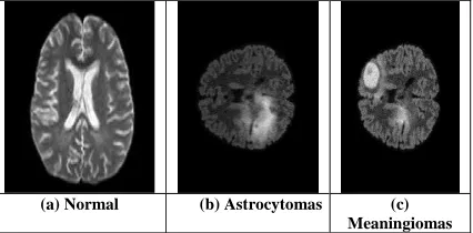
Many diagnostic imaging techniques can be performed for early detection of brain tumors such as Computed Tomography (CT), Positron Emission Tomography (PET) and Magnetic Resonance Imaging (MRI). Compared to all other imaging techniques, MRI is more efficient in brain tumor detection and identification, mainly due to the high contrast of soft tissues, high spatial resolution and since it does not produce any harmful radiation, and is a non invasive technique. Fig. 2(a),(b) and (c) shows the Magnetic Resonance Image (MRI) from BRATS database is categorized into three distinct classes as normal, Astrocytomas and Meaningiomas brain and it is considered for the implementation of DWT feature extraction and classification.
(a) Normal (b) Astrocytomas (c) Meaningiomas Fig. 2: MRI of the normal and abnormal images of the brain
This paper deals with brain tumor classification, which aims to identify the brain tumor types as normal or abnormal from the brain MRI images. The proposed approach is evaluated using BRATS 2014 dataset. Thus, the DWT features are extracted from the MRI image as a feature set. The extracted features are modeled by SVM, k-NN and Decision tree classifiers for training and testing. The rest of the paper is structured as follows. Section 2reviews related work. Section 3 provides an overview of the proposed approach. Section 4 describes the proposed feature extraction method and experimental results evaluating its performance on BRATS dataset are presented in Section 5. Finally, Section 6concludes the paper.
2. RELATED WORK
From the literature survey, initially
, it can be
concluded that, various research works have been performed in classifying MR brain images into normal and abnormal [1], [2]. Priyanka, BalwinderSingh [3] focused on survey of well-known brain tumor detection algorithms that have been proposed so far to detect the location of the tumor. The main concentration is on those techniques which use image segmentation to detect brain tumor. Image segmentation is the process of partitioning a digital image into multiple segments. R. J. Ramteke, KhachaneMonali Y [4] proposed a method for automatic classification of medical images in two classes Normal and Abnormal based on image features and automatic abnormality detection. KNN classifier is used for classifying image. K-Nearest Neighbour (K-NN) classification technique is the simplest technique conceptually and computationally that provides good classification accuracy. Khushboo Singh, SatyaVerma [5] proposed sophisticated classification techniques based onSupport Vector Machines (SVM) are proposed and applied to brain image classification using features derived. Shweta Jain [6] classifies the type of tumor using Artificial Neural Network (ANN) in MRI images of different patients with Astrocytomas type of brain tumor. The extraction of texture features in the detected tumor has been achieved by using Gray Level Co-occurrence Matrix (GLCM). Statistical texture analysis techniques are constantly being refined by researchers and the range of applications is increasing [7], [8], [9]. Gray level co-occurrence matrix method is considered to be one of the important texture analysis techniques used for obtaining statistical properties for further classification, which is employed in this research work. Probabilistic Neural Network is found to be superior over other conventional neural networks such as Support Vector Machine and Back propagation Neural Network in terms of its accuracy in classifying brain tumors [10]. Hence a wavelet and co occurrence matrix method based texture feature extraction and Probabilistic Neural Network for classification has been used in this method of brain tumor classification.
3. PROPOSED APPROACH
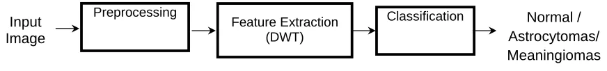
The general overview of the proposed approach is illustrated in Fig. 3. This approach uses the standard benchmark Brain Research and Analysis in Tissues (BRATS) tumor dataset [11] for the experiments. The input tumor images are smoothed by median filter. It is necessary to pre-process all the tumor images for robust feature extraction and classification. Then BRATS dataset divided into three classes (normal, Astrocytomas and Meaningiomas) for feature extraction process. The extracted features are modeled using SVM, k-NN and Decision tree for classification.
Fig. 3: Block diagram of the Proposed Approach
4. FEATURE EXTRACTION
The extraction of discriminative feature is most essential and vital problem with brain tumor classification, which
represents the meaningful information that is vital for further study. The ensuing sections present, the representation of the feature extraction method used in
this
work.
4.1. DWT for Tumor Classification
Discrete wavelet transform is a popular method in signal processing and has been used in various research fields. The main feature of DWT is the multi scale representation of a function. By using the wavelets, a given image can be analyzed at various levels of resolution. DWT converts an input series x0, x1, .., xm, into one high-pass
wavelet coefficient series and one low-pass wavelet coefficient series (of length n/2 each) as given below.
1 transformation is applied recursively on the low-pass series until the desired number of iterations is reached. In frequency domain, when the
MRI image is decomposed using two dimensional wavelet transform, four sub region [12]. These regions are: one low-frequency region LL (approximate component), and three high-frequency regions, namely LH (horizontal component), HL (vertical component), and HH (diagonal component), respectively. The LL image is generated by two continuous low-pass filters; HL is filtered by a high-pass filter first and a low-high-pass filter later; LH is created using a low-pass filter followed by a high-pass filter; HH is generated by two successive high-pass filters. Subsequent levels of decomposition follow the same procedure by decomposing the LL sub image of the previous level. Since
Input Image
Preprocessing
Feature Extraction (DWT)
the LL part contains most important information and discards the effect of noises and irrelevant parts, the LL part is adopted for further analysis. In the proposed work, two-level 2-D discrete wavelet decomposition is performed on the MRI images.
4.2 Support Vector Machine for Classification
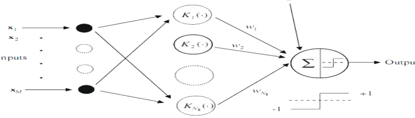
Support Vector Machine (SVM) [13] is based on the principle of structural risk minimization (SRM). Support vector machines can be used for pattern classification and nonlinear regression. It constructs a linear model to estimate the decision function using non-linear class boundaries based on support vectors. If the data are linearly separable, SVM trains linear machines for an optimal hyperplane that separates the data without error and into the maximum distance between the hyperplane and the closest training points. The training points that are closest to the optimal separating hyperplane are called support vectors. Fig. 4 shows the architecture of SVM. SVM maps the input patterns into a higher dimensional feature space through some nonlinear mapping chosen a priori. A linear decision
surface is then constructed in this high dimensional feature space. Thus, SVM is a linear classifier in the parameter space, but it becomes a nonlinear classifier as a result of the nonlinear mapping of the space of the input patterns into the high dimensional feature space.
4.2.1 SVM Principle:
Support vector machine (SVM) can be used for classifying the obtained data [14]. SVM are a set of related supervised learning methods used for classification and regression and they belong to a family of generalized linear classifiers. A feature vector (termed as pattern) is denoted by x=(x1, x2,… , xn) and its class label by y such that y = {+1,−1}. Therefore,
consider the problem of separating the set of n-training patterns belonging to two classes,
( , )
,
n,
{ 1,-1},
1,2,....,
i i i
x y x R y
i
n
(3)A decision function g(x) can correctly classify an input pattern x that is not necessarily from the training set.
Fig. 4: Architecture of the SVM (Ns is the number of support vectors).
4.2.2 SVM for Linearly Separable Data
A linear SVM is used to classify data sets which are linearly separable. The SVM linear classifier tries to maximize the margin between the separating hyperplane and the patterns lying on the maximal margins called support vectors. Such a hyperplane with maximum margin is called maximum margin hyperplane [14]. In case of linear SVM, the discriminant function is of the form:
( )
tg x
w x
b
(4)such that g(xi) ≥ 0 for yi = +1 and g(xi) < 0 for yi= −1. In
other words, training samples from the two different classes are separated by the hyperplane g(x) = wtx+b = 0. SVM
finds the hyperplane that causes the largest separation between the decision function values from the two classes. Now the total width
between two margins is 2/wtw, which is to be maximized.
Mathematically, this hyperplane can be found by minimizing the following cost function:
1
( )
2
t
J w
w w
(5)Subject to separability constraints
( )
1
1
( )
1
1
i i
i i
g x
for y
or
g x
for y
(6)Equivalently, these constraints can be re-written more compactly as
(
t) 1; 1, 2,....,
i i
y w x b
i
n
(7)For the linearly separable case, the decision rules defined by an optimal hyperplane separating the binary decision classes are given in the following equation in terms of the support vectors:
1
( , )
s i N
i i i
i
Y
sign
y
x x
b
(8)where Y is the outcome, yi is the class value of the training
example xi, and represents the inner product. The vector
the support vectors. In Eq. (8), b and
i are parameters that determine the hyperplane.4.2.3 SVM for linearly non-separable data:
For non-linearly separable data, it maps the data in the input space into a high dimension space
x
I
( )
x
H with kernel function
( ),
x
to find the separating hyperplane.4.2.4 Determining support vectors:
The support vectors are the (transformed) training patterns. The support vectors are (equally) close to hyperplane. The support vectors are training samples that define the optimal separating hyperplane and are the most difficult patterns to classify. Informally speaking, they are the patterns most informative for the classification task.
4.2.5 Inner product kernels:
SVM generally applies to linear boundaries. If a linear boundary is inappropriate, SVM can map the input vector into a high dimensional feature space. By choosing a non-linear mapping, the SVM constructs an optimal separating hyperplane in this higher dimensional space. The function K
is defined as the kernel function for generating the inner products to construct machines with different types of non-linear decision surfaces in the input space.
( , )
X x
i
( ). ( )
X
x
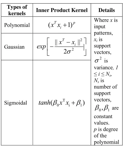
i (9)The kernel function may be any of the symmetric functions. There are several SVM kernel functions as given in Table 1.
Table 1: Types of SVM inner product kernels.
Types of
kernels Inner Product Kernel Details
Polynomial
(
x x
T i
1)
p Where input x is polynomial kernel of degree p and for the input pattern dimension of d is given byFor sigmoidal kernel and Gaussian kernel, the dimension of feature space vectors is shown to be infinite. Finding a suitable kernel for a given task is an open research problem. Given a set of images corresponding to N subjects for training, N SVMs are trained. Each SVM is trained to distinguish between all images of a single person and all other images in the training set. During testing, the class label l of a face pattern x can be determined using (11) from x to the SVM hyperplane corresponding to person i. The classification threshold is t, and the class label l = 0
stands for unknown.
4.3 k-Nearest Neighbour for Classification
The k-NN classifier ranks the test formula’s neighbors among the training vectors and uses the category labels of the k most similar neighbors to predict categories of the test formula [15], [16]. In traditional k-NN, the value k is fixed and usually determined experimentally. If the k is too large, big classes (a lot of members in the class) may dominate small ones. Incorrect categories may be assigned for multi-label classification. In the opposite, if k is too small, the advantages of this algorithm to make use of many experts will not be presented. Moreover, in multi-label classification, the test formula may not be assigned to all categories. It should be in k-NN algorithm, the most popular on similarity, i.e., cosine similarity, which can be calculated by the dot product between these two vectors. In case both vectors are normalized into the unit length, the value of similarity of the two vectors is in the range of 0 and 1.
( ) arg max
( , )
strategies could be taken to predict the category of a test formula. Two strategies that are widely used are listed as follows. Where fl is a test formula fj is one of the neighbors(k-NN) in the training set, z(fj , ck). 0,1 indicates whether fj
belongs to class ck in the set of classes C, and sim (fl, fj) is
the similarity function between fl and fj . For single-label
classification, the above equation means that the prediction will be a category that has the largest number of members in the k nearest neighbors. The Eq. (13) expresses that the category which has maximal sum of similarity (score), will be assigned. This strategy is thought to be more useful and is more widely used.
( ) argmax
( , ) ( , )
Decision tree is one of the preparatory learning algorithms that construct a classification tree to classify the data [17] and decision tree represents rules. The classification tree is made by recursive partitioning of feature space based on a training set. A decision tree is visual representation of a problem. A decision tree helps to decompose a complex problem into smaller and more manageable undertakings. Decision tree is a common and intuitive approach to classify a pattern through sequence of questions in which the next question depends upon the answer to current question. Decision tree analysis is a formal, structured approach to make decisions. It is based on the “divide and conquer” strategy.
There are two common issues for construction of decision trees [18]:
(a) Growth of the tree to accurately categorize the training dataset, and
(b) The pruning stage, whereby superfluous nodes and branches are removed in order to improve classification accuracy.
A decision tree is in the form of a tree structure, where each node is either:
1. A leaf node - indicates the value of the target class of examples, or
2. A decision node - specifies some test to be carried out on a single attribute-value, with two or more than two branches and each branch has a sub-tree. Decision trees are the commonly used method for pattern
classification. Decision tree is a common and intuitive approach to classify a pattern through sequence of questions in which the next question depends upon the answer to the current question. A decision tree is a visual representation of a problem. A decision tree helps to decompose a complex problem into smaller, more manageable undertakings. This allows the decision makers to make smaller determinations along the way to achieve the optimal overall decision. Decision tree analysis is a formal, structured approach to make decisions.
5. EXPERIMENTAL RESULTS
In this section, the proposed method is evaluated using BRATS tumor dataset. The experiments are carried out in MATLAB 2013a in Windows 7 Operating System on a computer with Intel Xeon Processor 2.40 GHz with 4 GB RAM. The obtained DWT features are fed to supervised classifiers such as SVM, K-NN and Decision tree to develop the model for each class, and these models are used to test the performance of the proposed features.
5.1 BRATS Dataset
Multimodal Brain Tumor Image Segmentation (BRATS) is a large dataset of brain tumor MR scans in which the relevant tumor structures have been delineated. In this work, 200 images are taken for evaluation is shown in the Fig. 5. For conducting the experiments, 120 images are taken as training samples and the remaining 80 images are considered fortesting
Fig. 5: Sample brain MRI images of the BRATS dataset: Normal (top row) and Abnormal (bottom row)
5.2 Quantitative Evaluation
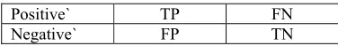
An efficient study of performance measure for classification tasks is presented in [19]. Precision (P), Recall (R) and F-measure (F) are the commonly used evaluation metrics and these measures are used to evaluate the performance of the proposed method. These measures provide the best perspective on classifiers performance for classification. Table 2 shows confusion matrix for classification.
Table 2: Confusion matrix for classification.
Predicted Outcomes
Positive Negative
Positive` TP FN
Negative` FP TN
(P) is calculated as in (14). The Recall (R) or Sensitivity is calculated as in (15).
Precision (P)
TP
TP FP
(14)Recall (R)
TP
TP FN
(15)F-Measure (F) 2
P R
P R
(16)
Accuracy (A)
TP TN
TP FP TN FN
(17)
Precision and Recall do not depend on TN, but only on the correct labeling of positive examples (TP) and the incorrect labeling of examples (FP and FN). These measures provide the most excellent perspective on classifier performance for brain tumor classification. The F-measure is a combined F-measure of precision and recall metrics and it is calculated as in (16). The Accuracy is calculated as in (17).
5.3 Results obtained with SVM
The confusion matrices of the SVM classifier on BRATS dataset is shown in Table 3, where diagonal of the table shows that accurate responses of tumor types.
The average recognition rate of SVM is 78.61%. In SVM, the normal class is classified well, where as in Astrocytomas class is confused with Meaningiomas class and vice versa. Thus, it needs further attention.
Table 3: Confusion matrix for SVM
Nor mal
Astrocyt omas
Meaningio mas
Normal 100 0.0 0.0
Astrocyto
mas 0.0 66.67 33.33 Meaningi
omas 0.0 30.83 69.17 5.4 Results obtained with k-NN
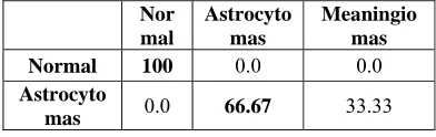
The confusion matrices of the k-NN classifier on BRATS dataset is shown in Table 4, where diagonal of the table shows that accurate responses of tumor types. The average recognition rate of k-NN is 88.89%. In k-NN, the normal and Meaningiomas classes are classified well and good, where as the Astrocytomas class is confused with Meaningiomas class as 33.33%.
Table 4: Confusion matrix for KNN
Nor mal
Astrocyto mas
Meaningio mas
Normal 100 0.0 0.0
Astrocyto
mas 0.0 66.67 33.33
Meaningio
mas 0.0 0.0 100
5.5 Results obtained with Decision Tree
The confusion matrices of the Decision Tree classifier on BRATS dataset is shown in Table 5, where diagonal of the table shows that accurate responses of tumor types. The average recognition rate of DT is 81.48%. In DT, the normal class is classified well, where as the Astrocytomas and Meaningiomas class are confused respectively. Thus, it needs further attention.
Table 5: Confusion matrix for Decision Tree
Nor mal
Astrocyt omas
Meaningio mas Normal 100 0.0 0.0 Astrocyt
omas 0.0 66.67 33.33 Meaning
iomas 0.0 22.22 77.78
Classifiers Precision Recall F-measure
SVM 66.67 66.67 66.52
K-NN 84.31 88.89 83.08 Decision
Tree 78.52 81.48 78.17 The quantitative evaluation results are tabulated in Table 6, which shows that the proposed approach has a higher precision, recall and F-measure for the k-NN classifier on BRATS dataset, when compared to SVM and DT classifiers. The overall performance of the proposed method with various classifiers on BRATS dataset is shown in Fig. 7.
Table 6: Performance measure of the BRATS dataset on SVM, k-NN and DT classifiers
Fig 7: Overall accuracy obtained for BRATS dataset on SVM, k-NN and DT classifiers
6. CONCLUSION AND FUTURE WORK
important texture features of tumor tissue and gives very promising results in classifying MR images. From the experimental results, it is observed that k-NN shows a classification accuracy of 88.89%, and demonstrated that the proposed feature method performs well and achieved good recognition results for tumor classification. It is observed from the experiments that the system could not distinguish Astrocytomas class with high accuracy and is of future interest.
7. REFERENCES
1. Ahmed kharrat, Karim Gasmi, et.al, “A Hybrid Approach for Automatic Classification of Brain MRI Using Genetic Algorithm and Support Vector Machine,” Leonardo Journal of Sciences, pp.71-82, 2010.
2. Ahmed Kharrat, Mohamed Ben Messaoud, et.al, “Detection of Brain Tumor in Medical Images,” International Conference on Signals, Circuits and Systems IEEE, pp.1-6, 2009.
3. Priyanka, Balwinder Singh. "A review on brain tumor detection using segmentation." International Journal of Computer Science and Mobile Computing (IJCSMC) 2.7 (2013): 48-54.
4. Ramteke, R. J., and Y. Khachane Monali. "Automatic medical image classification and abnormality detection using K-Nearest Neighbour." International Journal of Advanced Computer Research 2.4 (2012): 190-196.
5. Singh, Khushboo, and Satya Verma. "Detecting Brain Mri Anomalies By Using Svm Classification." International Journal of Engineering Research and Applications (IJERA) Vol. 2 (2012): 724-726.
6. Jain, Shweta. "Brain Cancer Classification N. Bhatia et al, Survey of Nearest Neighbor Techniques. International Journal of Computer Science and Information Security, Vol. 8, No. 2, 2010.
7. Leo Breiman, Jerome Friedman, Charles J Stone, and Richard A Olshen, Classification and regression trees, CRC press, 1984.
8. J. Ross Quinlan, “Induction of decision trees,” Machine learning, vol. 1, no. 1, pp. 81–106, 1986.
9. Marina Sokolova and Guy Lapalme, “A systematic analysis of performance measures for classification tasks,” Information Processing & Management, vol. 45, no. 4, pp. 427–437, 2009.n trees,” Machine learning, vol. 1, no. 1, pp. 81–106, 1986.
10. Marina Sokolova and Guy Lapalme, “A systematic analysis of performance measures for classification tasks,” Information Processing & Management, vol. 45, no. 4, pp. 427–437, 2009. 11. Using GLCM Based Feature Extraction in Artificial Neural
Network." International Journal of Computer Science & Engineering Technology 4.07 (2013).
12. Qurat-Ul-Ain, Ghazanfar Latif, “Classification and Segmentation of Brain Tumor using Texture Analyssis,” Recent Advances In Artificial Intelligence, Knowledge Engineering And Data Bases, pp 147-155, 2010.
13. Salim Lahmiri and Mounir Boukadoum,et.al., “Classification of Brain MRI using the LH and HL Wavelet Transform Sub-bands,” IEEE, 2011.
14. S. N. Deepa, et.al., “Second Order Sequential Minimal Optimization for Brain Tumor Classification,” European Journal of Scientific Research ISSN 1450-216X Vol.64 No.3, pp. 377-386, 2011.
15. Mohd Fauzi Bin Othman, Noramalina Bt Abdullah, et.al., “MRI Brain Classification using Support Vector Machine,” IEEE, 2011.
16. Menze, Bjoern H., et al. "The multimodal brain tumor image segmentation benchmark (BRATS)." IEEE Transactions on Medical Imaging 34.10 (2015): 1993-2024.
17. Sidra Batool Kazmi, Qurat ul Ain, and M. Arfan Jaffar, “Wavelets based facial expression recognition using a bank of neural networks,” in IEEE International Conference on Future Information Technology, 2010.
18. Nello Cristianini and John Shawe-Taylor, An introduction to support vector machines and other kernel-based learning methods, Cambridge university press, 2000.
19. Vladimir Naumovich Vapnik and Vlamimir Vapnik, Statistical learning theory, vol. 1, Wiley New York, 1998. 20. Keller, James M., Michael R. Gray, and James A. Givens. "A