Improvising Heart Attack Prediction System using Feature Selection and Data Mining Methods

(1)

! " #"# $ % %#

& ' ((( )

Improvising Heart Attack Prediction System using Feature Selection and Data Mining

Methods

B.Kavitha*

Lecturer

Department of Computer Applications, Karpagam University

Coimbatore, India [email protected]

R.Naveen Kumar

Lecturer

Department of Computer Applications, Karpagam University

Coimbatore, India [email protected]

Abstract: Medical diagnosis refers to the process of attempting to determine the identity of a possible disease. The identity of heart disease from various factors or symptoms is a multi-layered issue which is not free from false presumptions often accompanied by unpredictable effects. In this paper, we have proposed an efficient approach for the extraction of significant attributes from the heart disease warehouses for heart attack using forward selection method and have performed the classification of heart attack using data mining techniques. The data used in this paper is collected from UCI Machine Learning Repository Heart Disease dataset. The dataset consist of 303 records which have 14 attributes and after applying Correlation–based Feature Selection methods the original attributes was reduced to 6 potential attributes. We have investigated five data mining techniques such as J48, Naïve bayes, Logistic Regression, Classification via regression and Self-Organizing Map. The results shows that classification via regression have much better performance than other four methods and it is also observed that using feature selection method the performance of Logistic and Self Organizing Map has a notable improvement in their classification. It is observed that the classification accuracy increases better after dimensionality reduction.

Keywords:Data mining, weka, heart attack, j48, Naive bayes, logistic, classification, Regression, Self Organizing Map.

I. INTRODUCTION

Heart disease is a general name for a wide variety of diseases, disorders and conditions that affect the heart and sometimes the blood vessels. Heart disease is the number one killer of women and men in the world and most of them have myocardial infarctions. According to the National Heart, Lung, and Blood institute.

Types of heart disease includes angina, heart attack (myocardial infarction), atherosclerosis, heart failure, cardiovascular disease, and cardiac arrhythmias (abnormal heart rhythms). Other forms of heart disease include congenital heart defects, cardiomyopathy, infections of the heart, coronary artery disease, heart valve disorders, myocarditis and pericarditis.

Symptoms of heart disease vary depending on the specific type of heart disease. A classic symptom of heart disease is chest pain. However, with some forms of heart disease, such as atherosclerosis, there may be no symptoms in some people until life-threatening complications develop. Risk factors for developing heart disease include having hypertension, diabetes, high cholesterol (hypercholes terolemia, hyperlipidemia), obesity and a sedentary lifestyle. Peoples having ancestry, drinking excessive amounts of alcohol, having a lot of long-term stress, smoking and having a family history of a heart attack at an early age.

Extracting useful knowledge and providing scientific decision-making for the diagnosis and treatment of disease from the database increasingly becomes necessary. Data mining in medicine can deal with this problem. It can also improve the management level of hospital information and promote the development of telemedicine and community medicine. Because the medical information is characteristic of redundancy, multi-attribution, incompletion and closely related with time, medical data mining differs from other one.

The heart disease data warehouse consists of mixed attributes containing both the numerical and categorical data. These records are cleaned and filtered with the intention that the irrelevant data from the warehouse would be removed before mining process occurs. The aim of this paper is to predict the heart attack effectively by applying the attribute subset evaluator namely Correlation–based Feature Selection (CFS) subset Evaluator and the searching methods used are Best First Search, Genetic Search and Rank search. These three methods produce 6 significant attributes for classification. Using these significant attributes the classification of dataset is performed using J48, Naïve bayes, Logistic Regression, Classification via regression and Self-Organizing Map(SOM).

The remaining sections of the paper are organized as follows: In Section 2, a brief review of some of the works on heart disease diagnosis is presented. An introduction about the heart disease and its effects are given in Section 3. In Section 4 describtion about the dataset is produced. The section 5 explains the framework of the prosposed model. The extraction of significant attributes from heart disease data warehouse is detailed in Section 6. The classification methods used for predicting the heart attack is explained in Section 7. Estimation of model performance is shown in the Section 8. The experimental results are described in Section 9. The conclusions are summed up in Section 10.

II. RELATEDWORK

Numerous works in literature related with heart disease diagnosis using data mining and artificial intelligence techniques have motivated our work. Some of the related works are discussed in this section.

(2)

to develop the multi-parametric feature of HRV. Besides, they have assessed the linear and the non-linear properties of HRV for three recumbent positions, to be precise the supine, left lateral and right lateral position. Numerous experiments were conducted by them on linear and nonlinear characteri stics of HRV indices to assess several classifiers, e.g., Bayesian classifiers [5], CMAR (Classification based on Multiple Association Rules) [6], C4.5 (Decision Tree) [7] and SVM (Support Vector Machine) [8]. SVM surmounted the other classifiers.

A model Intelligent Heart Disease Prediction System (IHDPS) built with the aid of data mining techniques like Decision Trees, Naïve Bayes and Neural Network was proposed by Sellappan Palaniappan et al. [9]. The results illustrated the peculiar strength of each of the methodologies in comprehending the objectives of the specified mining objectives. IHDPS was capable of answering queries that the conventional decision support systems were not able to. It facilitated the establishment of vital knowledge, e.g. patterns, relationships amid medical factors connected with heart disease. IHDPS subsists well being web-based, user-friendly, scalable, reliable and expandable.

The prediction of Heart disease, Blood Pressure and Sugar with the aid of neural networks was proposed by Niti Guruet al. [10]. Experiments were carried out on a sample database of patients’ records. The Neural Network is tested and trained with 13 input variables such as Age, Blood Pressure, Angiography’s report and the like. The supervised network has been recommended for diagnosis of heart diseases. Training was carried out with the aid of back propagation algorithm. Whenever unknown data was fed by the doctor, the system identified the unknown data from comparisons with the trained data and generated a list of probable diseases that the patient is vulnerable to. In [11] Kiyong Noh et al. put forth a classification method for the extraction of multi-parametric features by assessing HRV from ECG, data preprocessing and heart disease pattern.

III. HEARTDISEASE

The term Heart disease encompasses the diverse diseases that affect the heart. Heart disease was the major cause of casualties in the United States, England, Canada and Wales as in 2007. Heart disease kills one person every 34 seconds in the United States [12]. Coronary heart disease, Cardiomyopathy and Cardiovascular disease are some categories of heart diseases. The term “cardiovascular disease” includes a wide range of conditions that affect the heart and the blood vessels and the manner in which blood is pumped and circulated through the body. Cardiovascular disease (CVD) results in severe illness, disability, and death [13]. Narrowing of the coronary arteries results in the reduction of blood and oxygen supply to the heart and leads to the Coronary heart disease (CHD). Myocardial infarctions, generally known as a heart attacks, and angina pectoris, or chest pain are encompassed in the CHD. A sudden blockage of a coronary artery, generally due to a blood clot results in a heart attack. Chest pains arise when the blood received by the heart muscles is inadequate [14].

IV. DATASETDESCRIPTION

Diagnosis of diseases is an important and difficult task in medicine. Detecting a disease from several factors or symptoms is a many-layered problem that also may lead to false assumptions with often unpredictable effects. Therefore, the attempt of using the knowledge and

experience of many specialists collected in databases to support the diagnosis process seems reasonable.

The dataset is collected for the UCI Machine Learning Repository [15]. This repository consists contains 4 databases concerning heart disease diagnosis. All attributes are numeric-valued. The data was collected from the the Clevelan database. The data was collected from Cleveland Clinic Foundation (cleveland.data)[16]. This database contains 76 attributes, but all published experiments refer to using a subset of 14 of them. In particular, this database is the only one that has been used by ML researchers to this date.

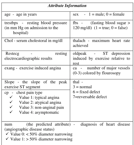
The "goal" field refers to the presence of heart disease in the patient. It is integer valued from 0 (no presence) to 4. Experiments with the Cleveland database have concentrated on simply attempting to distinguish presence (values 1, 2, 3, 4) from absence (value 0). Cleveland database consist of processed data. Number of Instances used for classification is 303. Total Number of Attributes: 76 (including the predicted attribute). While the databases have 76 raw attributes, only 14 of them are actually used. The Table I display 14 attributes used in this paper.

Table I. Dataset Attribute Information

Initially, the data warehouse is preprocessed to make the mining process more efficient. The data mining process of building Heart Attack prediction models is depicted in Fig. 1. In the first stage the dataset was collected from UCI Machine Learning Repository [15]. The data was collected from the Cleveland database [16]. In the second stage raw dataset is then preprocessed using the discretization method to convert the numeric values to the nominal values. In the third stage significant attribute selection is performed using CFS Subset Evaluator. The attribute evaluator performs the dimensionality reduction of dataset by reducing the number of attributes used for classification to 6 instead of 14. In the fourth stage five different classification algorithms are used to classify the dataset into healthy or sick. In the fifth stage the performance of each classification algorithms are discussed based on several evaluation models.

Attribute Information

(3)

V. PROPOSEDFRAMEWORK

Figure 1 Framework of the proposed model

VI. FEATURESELECTIONMEHTOD

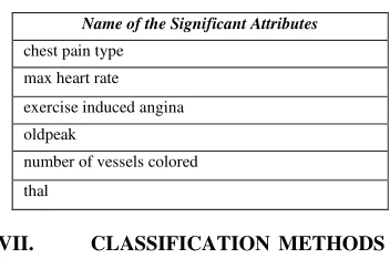
The feature selection is applied for dimensionality reduction while applying this it removes irrelevant, weakly relevant & redundant attribute. In this paper attributes selection is done using CFS Subset Evaluator and the three search method used are Best First Search, Rank search and Genetic Search [17]. All these search methods produces same 6 attributes as significant ones for predicting the Heart Attack. The attributes with high merit value is considered as potential attributes and used for classification. The significant 6 attributes used for the classification are listed in the Table II.

Table II. List of Significant Attributes

Name of the Significant Attributes

chest pain type

max heart rate

exercise induced angina

oldpeak

number of vessels colored

thal

VII. CLASSIFICATION METHODS

In this section the details of J48, Naïve bayes, Logistic Regression, Classification via regression and Self-Organizing Map (SOM) are discussed.

A. J48 classifier

A decision tree is a predictive machine-learning model that decides the target value (dependent variable) of a new sample based on various attribute values of the available data. The internal nodes of a decision tree denote the

different attributes, the branches between the nodes tell us the possible values that these attributes can have in the observed samples, while the terminal nodes tell us the final value (classification) of the dependent variable.

The J48 Decision tree [18] classifier follows the following simple algorithm. In order to classify a new item, it first needs to create a decision tree based on the attribute values of the available training data. So, whenever it encounters a set of items (training set) it identifies the attribute that discriminates the various instances most clearly. This feature that is able to tell us most about the data instances so that we can classify them the best is said to have the highest information gain. Now, among the possible values of this feature, if there is any value for which there is no ambiguity, that is, for which the data instances falling within its category have the same value for the target variable, then we terminate that branch and assign to it the target value that we have obtained.

For the other cases, we then look for another attribute that gives us the highest information gain. Hence we continue in this manner until we either get a clear decision of what combination of attributes gives us a particular target value, or we run out of attributes. In the event that we run out of attributes, or if we cannot get an unambiguous result from the available information, we assign this branch a target value that the majority of the items under this branch possess.

Now that we have the decision tree, we follow the order of attribute selection as we have obtained for the tree. By checking all the respective attributes and their values with those seen in the decision tree model, we can assign or predict the target value of this new instance. The above description will be more clear and easier to understand with the help of an example. Hence, let us see an example of J48 decision tree classification.

J48 employs two pruning methods:

[a] The first is known as subtree replacement. This means that nodes in a decision tree may be replaced with a leaf basically reducing the number of tests along a certain path. This process starts from the leaves of the fully formed tree, and works backwards toward the root. [b] The second type of pruning used in J48 is termed sub

tree rising. In this case, a node may be moved upwards towards the root of the tree, replacing other nodes along the way. Sub tree rising often has a negligible effect on decision tree models. There is often no clear way to predict the utility of the option, though it may be advisable to try turning it off if the induction process is taking a long time. This is due to the fact that sub tree rising can be somewhat computationally complex.

B. Naive Bayes Model

A Naive Bayes classifier [19] is a simple probabilistic classifier based on applying Bayes' theorem with strong independence assumptions. A more descriptive term for the underlying probability model would be "independent feature model". In spite of their naive design and apparently over-simplified assumptions, naive Bayes classifiers often work much better in many complex real-world situations than one might expect. Recently, careful analysis of the Bayesian classification problem has shown that there are some theoretical reasons for the apparently unreasonable efficacy of naive Bayes classifiers.

Naive Bayes classifiers assume that the effect of a variable value on a given class is independent of the values of other variable. This assumption is called class conditional independence. This assumption is a fairly strong assumption

UCI Repository Heart Attack Dataset

Preprocessing discretization

Feature selection

Classification models

Evaluation & Comparison results

(4)

and is often not applicable. However, bias in estimating probabilities often may not make a difference in practice -- it is the order of the probabilities, not their exact values that determine the classifications. Studies comparing classifica tion algorithms have found the Naive Bayesian classifier to be comparable in performance with classification trees and with neural network classifiers. They have also exhibited high accuracy and speed when applied to large Bayes Theorem

[a] Let X be the data record (case) whose class label is unknown. Let H be some hypothesis, such as "data record X belongs to a specified class C." For classification, we want to determine P (H|X) -- the probability that the hypothesis H holds, given the observed data record X.

[b] P (H|X) is the posterior probability of H conditioned on X. For example, the probability that a fruit is an apple, given the condition that it is red and round. In contrast, P(H) is the prior probability, or apriori probability, of H. In this example P(H) is the probability that any given data record is an apple, regardless of how the data record looks. The posterior probability, P (H|X), is based on more information (such as background knowledge) than the prior probability, P(H), which is independent of X. [c] Similarly, P (X|H) is posterior probability of X

conditioned on H. That is, it is the probability that X is red and round given that we know that it is true that X is an apple. P(X) is the prior probability of X, i.e., it is the probability that a data record from our set of fruits is red and round. Bayes theorem is useful in that it provides a way of calculating the posterior probability, P(H|X), from P(H), P(X), and P(X|H).

Bayes theorem is:

P (H|X) = P (X|H) P (H) / P(X) (1)

C. Logistic Regression

Logistic regression (LR)[20] is a venerable, but capable probabilistic binary classifier. LR is well-understood, mature and comfortable =) trusted LR accuracy is comparable to new-fangled state-of-the-art SVMs .LR can be as fast or faster than linear SVMs

An explanation of logistic regression begins with an explanation of the logistic function:

(2)

A graph of the function is shown in figure 1. The input is z and the output is ƒ(z). The logistic function is useful because it can take as an input any value from negative infinity to positive infinity, whereas the output is confined to values between 0 and 1. The variable z represents the exposure to some set of independent variables, while ƒ(z) represents the probability of a particular outcome, given that set of explanatory variables. The variable z is a measure of the total contribution of all the independent variables used in the model and is known as the log it.

The variable z is usually defined as

(3) Where 0 is called the "intercept" and 1, 2, 3, and so on, are called the "regression coefficients" of x1, x2, x3

respectively. The intercept is the value of z when the value of all independent variables is zeros (e.g. the value of z in someone with no risk factors). Each of the regression coefficients describes the size of the contribution of that risk factor. A positive regression coefficient means that the explanatory variable increases the probability of the outcome, while a negative regression coefficient means that the variable decreases the probability of that outcome; a large regression coefficient means that the risk factor strongly influences the probability of that outcome; while a near-zero regression coefficient means that that risk factor has little influence on the probability of that outcome.

Logistic regression is a useful way of describing the relationship between one or more independent variables (e.g., age, sex, etc.) and a binary response variable, expressed as a probability, that has only two possible values, such as death ("dead" or "not dead")

D. Support Vector Machine

A self-organizing map (SOM)[21] or self-organizing feature map (SOFM) is a type of artificial neural network that is trained using unsupervised learning to produce a low-dimensional (typically two-dimensional), discretized representation of the input space of the training samples, called a map. Self-organizing maps are different from other artificial neural networks in the sense that they use a neighborhood function to preserve the topological properties of the input space.

There are two ways to interpret a SOM. Because in the training phase weights of the whole neighborhood are moved in the same direction, similar items tend to excite adjacent neurons. Therefore, SOM forms a semantic map where similar samples are mapped close together and dissimilar apart. This may be visualized by a U-Matrix (Euclidean distance between weight vectors of neighboring cells) of the SOM.

The other way is to think of neuronal weights as pointers to the input space. They form a discrete approximation of the distribution of training samples. More neurons point to regions with high training sample concentration and fewer where the samples are scarce.

SOM may be considered a nonlinear generalization of Principal components analysis (PCA)[22]. It has been shown, using both artificial and real geophysical data, that SOM has many advantages over the conventional feature extraction methods such as Empirical Orthogonal Functions (EOF) or PCA.

Originally, SOM is not a solution to optimization problems. Nevertheless, there are several attempts to modify definition of SOM and to formulate an optimization problem which gives the similar results. For example, Elastic maps use mechanical metaphor of elasticity and analogy of the map with elastic membrane and plate.

E. ClassifierviaRegression

For learning reductions we have been concentrating on reducing various complex learning problems to binary classification [23]. This choice needs to be actively questioned, because it was not carefully considered.

Binary classification is learning a classifier c:X -> {0,1} so as to minimize the probability of being wrong, Prx,y~D(c(x) <> y).

(5)

judgment must at least partially be made on non theoretical grounds because (essentially) we are evaluating a choice between two axioms/assumptions.

These two primitives are significantly related. Classification can be reduced to regression in the obvious way: you use the regressor to predict D(y=1|x), then threshold at 0.5. For this simple reduction a squared error regret of r implies a classification regret of at most r0.5. Regression can also be used to reduce to classification using the Probing algorithm. (This is much more obvious when you look at an updated proof) Under this reduction, a classification regret of r implies a squared error regression regret of at most r.

Both primitives enjoy a significant amount of prior work with (perhaps) classification enjoying more work in the machine learning community and regression having more emphasis in the statistics community.

VIII. ESTIMATIONOFMODELPERFORMANCE

Weka 3.6[24] data mining tool kit is used for analyzing the results. The classification models can be evaluated using misclassification error rate and the area under ROC curve. The classification models can be evaluated using 10 fold cross validation method, confusion matrix, ROC curve and other statistical Methods.

A. Confusion Matrix

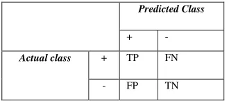
One of the methods to evaluate the performance of a classifier is using confusion matrix the number of correctly classified instances is sum of diagonals in the matrix; all others are incorrectly classified. The following terminology is often used when referring to the counts tabulated in a confusion matrix

Table III. AConfusion matrix for a binary classification problem in which the classes are not equally important

Predicted Class

+ -

Actual class + TP FN

- FP TN

[a] The True Positive (TP) [25]: corresponds to the number of positive examples correctly predicted by the classification model.

[b] The False Negative (FN) [25]: corresponds to the number of positive examples wrongly predicted as negative by the classification model.

[c] The False Positive (FP) [25]: corresponds to the number of negative examples wrongly predicted as positive by the classification model.

[d] The True Negative (TN) [25]: corresponds to the number of negative examples correctly predicted by the classification model.

B. Fold Cross Validation:

[a] First step: data is split into 10 subsets of equal size (usually by random sampling).

[b] Second step: each subset in turn is used for testing and the remainder for training.

[c] The error estimates are averaged to yield an overall error estimate

C. The Receiver Operating Characteristic Curve (ROC)

ROC[25] curve, is a graphical plot of the sensitivity vs. (1 − specificity) for a binary classifier system as its discrimination threshold is varied.

[a] X axis shows percentage of false positives (FP) in the sample.

[b] Y axis shows percentage of true positives (TP) in the sample

D. Other statistical Methods

Kappa Statistics: The kappa measure of agreement is the ratio K = P(A) - P(E) / (1 - P(E)) (4)

Where, P (A) is the proportion of times the k raters agree, and P (E) is the proportion of times the k raters are expected to agree by chance alone.

Mean Absolute Error: In statistics, the mean absolute error is a quantity used to measure how close forecasts or predictions are to the eventual outcomes. The mean absolute error (MAE) is given by

(5)

The mean absolute error is an average of the absolute errors ei = fi − yi, where fi is the prediction and yi the true

Root Mean Squared Error (RMSE): It is a frequently-used measure of the differences between values predicted by a model or an estimator and the values actually observed from the thing being modeled or estimated.

Relative Absolute Error:The relative absolute error Ei of an

individual program i is evaluated by the equation):

(6)

where P(ij) is the value predicted by the individual program i for sample case j (out of n sample cases); Tj is the target

value for sample case j; and is given by the formula:

(7)

For a perfect fit, the numerator is equal to 0 and Ei = 0. So, the Ei index ranges from 0 to infinity, with 0 corresponding to the ideal.

Root Relative Squared error:The root relativesquared error

Ei of an individual program i is evaluated by the equation:

(8)

IX. PERFORMANCEEVALUATIONAND

RESULT

(6)

classification in efficient manner. The Tables IV, V, VI and VII Shows the performance of five classification methods based on correctly and incorrectly classified Instances, Kappa statistic and Mean absolute error, Root Mean Square Error and Relative Absolute Error, Root Relative Squared error and Time taken to build the models respectively. The comparison is performed for both 14 and 6 attributes.

Table IV. Comparison of five models based on Correctly and Incorrec tly classified Instancestly classified Instances

Classifcation

NaiveBayes 84.1584 83.8284 15.8416 16.1716 Classification

Via Regression 85.4785 84.1584 14.5215 15.8416

J48 77.2277 76.8977 22.7723 23.1023

Logistic 83.1683 84.1584 16.8317 15.8416

SMO 82.8383 84.4884 17.1617 15.5116

Kappa statistic Mean absolute error

14 6 14 6

NaiveBayes 0.6795 0.6714 0.1877 0.1959 Classification

Via Regression 0.7055 0.6787 0.2457 0.2523

J48 0.539 0.5309 0.286 0.2855

Logistic 0.6601 0.6806 0.2164 0.2278

SMO 0.652 0.6852 0.1716 0.1551

Table VI. Comparison of five models based on Root mean squared error and Relative absolute error

Via Regression 0.3401 0.3532 49.5219 50.8664

J48 0.4303 0.4165 57.646 57.5551

Logistic 0.3447 0.3469 43.6261 45.9212

SMO 0.4143 0.3938 34.5936 31.2673

Table VII. Comparison of five models based on Relative absolute error and Time taken to build model

Classifcation time consuming process that requires a deep understanding of statistics. The result of Tables IV, V, VI and VII shows that both in 14 and 6 attributes Classification via Regression outperforms the remaining algorithms. It is observed that after performing feature reduction method J48, Logistic Regression and SMO has a significant improvement in their classification but NaiveBayes has a poor performance. The fig 2 depicts the performance of the classification methods

ROC curve of 5 classification Modles using 6 attributes

X. CONCLUSION

In this contribution CFS Subset Attribute Evaluator is used to rank the features extracted for predicting heart attack. From the result, it is observed that after reducing the dimensionality from 14 attributes to 6 attributes. The performance of ClassificationviaRegression outperforms the remaining four algorithms J48, Logistic Regression and SMO has a significant improvement in their classification but NaiveBayes has a poor performance. Time Taken by this algorithm is very less. Results showed that the classification accuracy is increased using 6 attributes than the 14 attributes. The Time Taken by all algorithms is considerably less using 6 attributes. It is observed that the classification accuracy increases better after dimensionality reduction.

XI. REFERENCES

[1] Anamika Gupta, Naveen Kumar, and Vasudha Bhatnagar, "Analysis of Medical Data using Data Mining and Formal Concept Analysis", Proceedings Of World Academy Of Science, Engineering And Technology,Vol. 6, June 2005,

[2] Frank Lemke and Johann-Adolf Mueller, "Medical data analysis using self-organizing data mining technolo gies," Systems Analysis Modelling Simulation, Vol. 43, No. 10, pp: 1399 -1408, 2003.

(7)

[4] Heon Gyu Lee, Ki Yong Noh, Keun Ho Ryu, “Mining Biosignal Data: Coronary Artery Disease Diagnosis using Linear and Nonlinear Features of HRV,” LNAI 4819: Emerging Technologies in Knowledge Discovery and Data Mining, pp. 56-66, May 2007.

[5] Chen, J., Greiner, R., “Comparing Bayesian Network Classifiers”, In Proc. of UAI-99, pp.101– 108, 1999

[6] Li, W., Han, J., Pei, J., “CMAR: Accurate and Efficient Classification Based on Multiple Association Rules”, In: Proc. of 2001 Interna’l Conference on Data Mining. 2001.

[7] Quinlan, J., “C4.5: Programs for Machine Learning”, Morgan Kaufmann, San Mateo 1993.

[8] Cristianini, N., Shawe-Taylor, J. “An introduction to Support Vector Machines”, Cambridge University Press, Cambridge, 2000.

[9] Sellappan Palaniappan, Rafiah Awang, "Intelligent Heart Disease Prediction System Using Data Mining Techniques", IJCSNS International Journal of Computer Science and Network Security, Vol.8 No.8, August 2008

[10] .Niti Guru, Anil Dahiya, Navin Rajpal, "Decision Support System for Heart Disease Diagnosis Using Neural Network", Delhi Business Review , Vol. 8, No. 1 (January - June 2007.

[11] Kiyong Noh, Heon Gyu Lee, Ho-Sun Shon, Bum Ju Lee, and Keun Ho Ryu, "Associative Classification Approach for Diagnosing Cardiovascular Disease", springer,Vol:345 , pp: 721-727, 2006

[12] “Heart disease” from http://wikipedia.org

[13] "Hospitalization for Heart Attack, Stroke, or Congestive Heart Failure among Persons with Diabetes", Special report: 2001 – 2003, New Mexico

[14] Chen, J., Greiner, R.: Comparing Bayesian Network Classifiers. In Proc. of UAI-99, pp.101–108, 1999.

[15] Heart attack dataset from http://archive.ics.uci.edu/ml/ datasets/Heart+Disease

[16] Robert Detrano, M.D., Ph.D, V.A. Medical Center, Long Beach and Cleveland Clinic Foundation

[17] Guyon, I., Weston, J., Barnhill, S., Vapnik, V.: Gene selection for cancer classification using support vector machine. Machine Learning 46(1-3), 389–422 (2002)

[18] J48classifier,http://www.d.umn.edu/~padhy005/chapter 05.html

[19] Harry Zhang "The Optimality of Naive Bayes". FLAIRS 2004 conference

[20] S.B. Kotsiantis, Supervised Machine Learning: A Review of Classification Techniques, Informatica 31(2007) 249-268, 2007

[21] Ultsch A (2003). U*-Matrix: a tool to visualize clusters in high dimentional data. University of Marburg, Department of Computer Science, Technical Report Nr. 36:1-12

[22] Yin H. Learning Nonlinear Principal Manifolds by Self-Organising Maps, In: Gorban A. N. et al. (Eds.), LNCSE 58, Springer, 2007 ISBN 978-3-540-73749-0

[23] http://hunch.net/?p=211

[24] WEKA: Data Mining Software in Java (2008), http://www.cs.waikata.ac.nz/ml/weka