! " #
$#$ !% & &$
' ( ))) *
Face Detection in Multi-Resolution Images
Ramesh Kumar Jallu
Department of Mathematical and Computational Sciences National Institute of Technology, Karnataka,
Mangalore, India [email protected]
Jidesh. P*
Department of Mathematical and Computational Sciences National Institute of Technology, Karnataka,
Mangalore , India [email protected]
Abstract: A face recognition method is proposed in this paper which can handle the images with different resolution, pose and illumination. The results are provided to compare the performance of the proposed method with some of the existing methods.
Keywords: Multi-resolution; Face Recognition; Face detection; PCA; LDA;
I. INTRODUCTIONTOFACERECOGNITION
Feature extraction is one of the main steps in face-detection and recognition process. Many methods have been proposed in literature for efficient and accurate face recognition process. The powerful tools like Principle component analysis (PCA) and linear discriminant analysis (LDA) are widely used for dimensionality reduction, feature extraction respectively and have been proved to be very successful in face recognition process. The possibility of applying PCA for an efficient face recognition process was first explored by M.Truk [1]. Though PCA is good enough for an un-biased face recognition process, it fails to recognize the faces with different pose and varying illumination characteristics. It is widely known that LDA based techniques can perform with desirable accuracy even with the pose and the illumination issues. Alex M. in [6] numerically compared the performance of PCA and LDA. Though PCA and LDA are quite efficient in feature extraction, it is of big concern among the research community on when to use what. This issue was reasonably addressed in [9] by the authors. In this paper the authors conclude that, if the number of samples per class is large the LDA would be the suitable option whereas if the number of samples per class is less then PCA would outperform LDA due to its light computational complexity. Further the possibility of using Support vector machine (SVM) and Independent component analysis (ICA) for classification and matching were analyzed, the details can be found in [11,2] and [7,12] respectively. The face recognition process involves a feature extraction, feature classification and matching here we propose to use a combination of PCA and LDA for classification and matching. The recognition process is demonstrated in the block diagram shown in Figure 1.
Fig.1. Face detection and recognition process
This paper is organized in four sections. In section 1 we provide a survey on the existing methods for face recognition in the literature and we explain in detail about the application
of LDA and PCA for face recognition process. In section 2 we explain about the proposed work. Section 3 gives a detailed analysis on the experiential results and discussions. We conclude this work in Section 4.
A. Principal Component Analysis (PCA)
PCA is one of the most successful techniques widely used in dimensionality reduction, data compression and feature extraction. The main aim of PCA is to preserve as much information as possible using fewer coefficients.
The advantages of PCA are 1) storing the training images in the form of their projections on the reduced basis. 2) Reduction of noise, because we store the principal components only. Hence features like background with small variation will be automatically ignored. The main idea behind PCA for face recognition is construction of one dimensional feature space from a two dimensional facial image, it is called as eigenspace projection. Where the eigen-space corresponds to a space spanned by the eigen-vectors of the covariance matrix derived from the dataset. PCA is explained in the following steps:
1) Consider M training images I1, I2… IM in a data set. It is assumed that the face is centered in the input images.
2) Represent each image I as a column vector i. Where each
Ii is an N X N matrix and i is N2x 1 matrix.
3) Find the average of all images.
4) Subtract the mean face ( ) from each face vector i to get
set of vectors i. The purpose of subtracting the mean image
from each image vector is to leave only the distinguishing features from each face and removing the common information.
i i
Φ = Γ − Ψ
(1) 5) Find the covariance matrix C:
C
=
AA
T (2)6) We now need to calculate the eigenvectors ui of C, however
note that C is a N2 x N2 matrix and it would return N2 eigenvectors each are N2 x 1 dimensional vectors. Generally for an image this number is large.
7) Instead of the matrix AAT consider the matrix ATA. A is
N2
x
M matrix, thus ATA is Mx
M matrix. If we find the eigenvectors of this matrix, it would return only M eigenvectors, each of Mx
1 dimension.Fig.2. (a) The First row shows the face images in the database (b) The Second row shows eigenfaces corresponding to each face in the database obtained after applying PCA (c) The Third row shows Fisher faces corresponding to each face in the database obtained after applying LDA
Let us call these eigenvectors vi’s. Then the eigenvectors
corresponding to the matrix AAT can be written as:
u
i=
Av
i (3) This implies that using these ui’s we can calculate the Mlargest eigenvectors of AAT. Note that M<<N2 as M is the number of training images.
8) Find the eigenvectors of C in (2). Note that there will be M eigenvectors.
9) Select K eigenvectors corresponding to the highest eigenvalues based on the desired accuracy. The eigenvectors corresponding to non-zero eigenvalues only chosen because they are linearly independent and can form a basis for the space spanned by these eigenvectors. Figure.2 shows eigenfaces corresponding best eigenvectors.
10) Find weights for eigenvectors found in step 9. These eigenvectors form a basis. Each eigenvector forms an eigenface. Now each face in the training set minus the mean ( i) can be represented as a linear combination of these
eigenvectors ie.
Φ = Σ
i Kj=1w u
j j (4)(Since we have chosen K best eigenvectors). Here wj is weight
and can be calculated using
w
j=
u
TjΦ
i,
i
=
1, 2,...,
M
(5)Each normalized training image is represented in this basis as a vector
Ω =
i[
w w
1,
2.
.
.
w
k]
T (6)Where i = 1, 2... M. This means that we have to calculate such a vector corresponding to every image in the training set and store them as templates.
The recognition process is as follows.
Now consider we have found out the eigenfaces for the training images, their associated weights after selecting a set of most relevant eigenfaces and stored these vectors corresponding to each training image. If an unknown probe face is to be recognized then:
1) We normalize the incoming probe as
Φ = Γ − Ψ
(7) 2) We then project this normalized probe onto the eigenspace (a space spanned by eigenvector) and find out the weights usingT
i i
w
=
u
Φ
(8) 3) The normalized probe can then simply be represented as1 2
...
[
w w
,
w
k]
Tfound using the following equation which defines a residual norm:
,
1, 2,...,
iEd
=
min
Ω − Ω
i
=
M
(10)Where ||.|| denotes the Euclidean norm. The vector (in the database) having the minimum residual norm is assumed to be matching more with the input vector. If Ed < , where is a threshold chosen heuristically, then we can say that the probe image is recognized as the image with which it gives the lowest score. If Ed > ; then the probe does not belong to the database hence a possible mismatch is alarmed.
The main disadvantages of PCA are: (1) It provides little quantitative information and visualization implications (2) There is hardly any way to discriminate between variance due to object of interest and variance due to noise or background (3) It is difficult to evaluate the covariance matrix accurately and computing complexity is high (4) It can only process the faces have the same face expression. In order to solve the problems 3, 4, a new face recognition method called SPCA (Statistical Principal Component Analysis Method) [13] has been proposed. The motivation of LDA is to find out an axis, on which the data points of different classes are far from each other while equiring data points of the same class to be close to each other.
B. Linear Discriminant Analysis (LDA)
LDA is mainly used in classification problems. LDA deals with scatter matrices like within-class (Sw) and
between-class (Sb) scatter matrices. This method maximizes the ratio of
between class variance to the within-class variance in any particular data set thereby guaranteeing maximal separability. The use of LDA for data classification is applied to classification problem in speech recognition. LDA provides better classification compared to PCA. The prime difference between LDA and PCA is that PCA does feature classification whereas LDA does data classification. In PCA, the shape and location of the original data sets changes when transformed to a different space whereas LDA does not change the location but only tries to provide more class separability and draw a decision region between the given classes. This method also helps to better understand the distribution of the feature data. There are two main areas where discriminant analysis is useful 1) Classification 2) Feature selection. The basic idea of LDA is to find a linear transformation such that feature clusters are most separable after the transformation. This can be achieved through scatter matrix analysis.
LDA is explained briefly as follows. 1) Let there are m classes C1, C2 …Cm.
2) Find the mean vector i of class i, i = 1, 2…m.
3) Calculate total number of samples.
Let 1 m i i
M
M
==
(11)Where Mi be the number of samples within class i, i=1, 2…m.
4) Find the within-class scatter matrix
1 1
(
)(
)
i
M
T
w j i j i
i m
j
S
y
µ
y
µ
= =
=
−
−
(12)5) Find the between-class scatter matrix
1
(
)(
)
Tb i
i m
i
S
µ
µ µ
µ
=
=
−
−
(13)Where 1
1
(
)
i m iMean of entire data set
C
µ
µ
=
=
(14)LDA computes a transform that maximizes the between-class scatter while minimizing the within-class scatter,
i.e. maximize
(
)
(
)
b
w
det S
det S
A detailed description on LDA can be found in [4].
C. Support Vector Machines (SVM)
Support Vector Machine (SVM) is one of the widely used techniques in pattern classification problems especially in face-recognition. SVMs are essentially developed to solve a two class pattern recognition problem. A SVM finds a hyperplane that separates the largest possible fraction of points of the same class on the same side, while maximizing the distance from either class to the hyperplane. We can apply SVM to multi-class problems. The process of face recognition using SVM is as follows.
1) Feature extraction:
Firstly, PCA is performed on the training face images. After applying PCA the training face images are projected onto the eigenspace. Projection coefficients are taken as the features to the corresponding training faces. Then, the projection coefficients are normalized by
(
i i)
i ix
x
µ
σ
′−
=
(15)Where xi is the ith projection coefficient, i and i are the mean
and standard deviation respectively. 2) Recognition:
Firstly, an incoming face image projected onto the eigenfaces faces obtained in training phase. Generate a feature vector by taking projection coefficients of the new face. Projection coefficients are normalized using (15), and mean and deviation are obtained from the training samples. The methods like binary tree or distance measure are widely used for recognizing the incoming face. Further details found can be found in [2].
Like the other methods explained above, SVM learning has also been applied for the face detection. But the main drawbacks of this technique are (i) training on adequately large datasets is hard (ii) SVM does not perform well when occlusions are present in the datasets. Due to these reasons the SVM is generally not used for face recognition process.
II. PROPESEDMETHOD
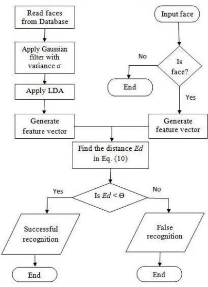
in Fig.3 explains the process of recognizing low-resolution face. All the facts discussed above prompted us to think in the direction of proposing a method which performs well even in case of the images with different resolutions. It is not always guaranteed that all the images we receive for recognition are of same resolution. It is quite possible to have the same image with different sampling rate which causes the image to be of different resolution depending on the sampling rate. So in most of the practical scenarios one has deal with resolution images. In this works we handle the multi-resolution scenario by storing images at three different resolutions in the database so even if the input image is of different resolution the method will guarantee a possible match better than that of the other methods. So in general the input face image may be of low resolution, in such cases we compare the low resolution images with this input face by using LDA.
Fig.3. Face detection and recognition process in case of multi-resolution images.
A. Process of recognition for low resolution face images 1) Get the low resolution image I which is to be recognized. 2) Apply Gaussian filter on trained set of images.
2 2 2
( ) 2 2
1
( , )
2
x y
G x y
e
σπσ
− +
=
(16) [image:4.612.69.283.242.537.2]With zero mean, variance 2, where x,y are special coordinates. I =I*G(x,y), where * is convolution operation. 3) Apply LDA on set of images obtained in second step. Fig. 3 shows the process of proposed method.
III. EXPERMENTALRESULTSANDDISCUSSIONS
In this section, we investigate the performance of our proposed method for multi-resolution face recognition. All the functions in these methods are implemented in MATLAB,
[image:4.612.314.546.260.527.2]version 7.5.0.342(R2007b). The performance is compared with PCA and LDA. The results presented in this section are obtained for the face images from IFD (Indian Face database) [3, 5]. This database contains over 700 color images of 61 persons of 22 female and 39 male. Each image is of dimension 640 x 480. There are eleven different images for each person. These images are of different pose and illumination and all are centered in middle and taken using the same camera. In our experiment we consider seven faces corresponding to each person. We used 150 images, 70 (M) for training and 80 for testing and 42(K) best non-zero eigenvectors corresponding to = 0:4311 have been taken for recognition task. In Fig. 2, the first row shows the test images, second row shows the eigenfaces obtained by PCA and the third rows show fisher faces obtained using LDA. The results obtained by PCA, LDA and proposed method are presented in Table I. It is observed that if the variance 2 increases recognition rate decreases because the resolution of the image is getting decreased.
Fig.4. Error recognition rate in PCA and LDA
Fig.5. Recognition rate in case of multi-resolution
One can observe that the proposed method works well with different resolution levels (for varying 2 compared to the other methods. Figure 4 shows the error rate between PCA and LDA. If the number of samples increases per image error rate decreases. It goes to almost zero if the number of images per face is large. Figure 5 shows a plot of recognition rate versus variance 2: It can be observed that the recognition rate of our
method increases and achieves best result rate in case of multi-resolution.
Table I. Recognition Percentage of Multi-resolution images in PCA, LDA and Proposed method
Variance
2 PCA (%) LDA (%) Proposed Method (%)
0.25 78 80 84
0.5 72 74 78.5
[image:4.612.317.553.678.741.2]1 60 62.5 67
2 56.5 58.5 62
3 53 55 59.5
IV. CONCLUSION
An efficient face recognition method is proposed which combines PCA and LDA techniques to address the issues arose due to the pose and illumination characteristics of the image, further the method is scaled to withstand the setbacks caused due to the multi-resolution images for the recognition process. The quantitative results provided are sufficient to substantiate the fact that; the proposed method works well compared to the existing methods in the literature.
V. REFERENCES
[1] M. Turk and A. Pentland, “Eigenfaces for Recognition’, J. Cognitive Neuroscience, vol. 3, no. 1, pp. 71-86, 1991. Recognition”,In Advances in Neural Information Processing Systems 11, pp. 803-809, 1998.
[2] Guodong Guo, Stan Z.Li and Kap Luk Chan,“Support vector machines for face recognition’,Journal on image and vision computing, vol. 19, pp.631-638, 2001.
[3] http://web.mit.edu/emeyers/www/facedatabases.html#rich ard(list of all databases).
[4] Juwei Lu, Plataniotis, K.N, Venetsanopoulos, A.N, “Face recognition using LDA-based algorithms”, IEEE Transactions on Neural Networks, vol. 14, pp.195-200, 2003.
[5] Indian face database http://vis-www.cs.umass.edu/~vidit/IndianFaceDatabase/ [6] Aleix M. Martinez and A. C. Kak, “PCA versus LDA”,
IEEE Transaction on Pattern Analysis and Machine Intelligence, 23(2):pp.228-233, 2001.
[7] Bartlett.M.S, Movellan.J.R, Sejnowski.T.J,“Face recognition by independent component analysis”,IEEE Transactions on Neural Networks, vol.13, pp.1450-1464, 2002.
[8] Sang-Woong Lee, Jooyoung Park,Seong-Whan Lee,“Low resolution face recognition based on support vector data description”, The Journal of The Pattern Recognition Society, 39(2006) pp.1809-1812.
[9] W . Zhao, R. Chellappa, A. Rosenfeld, P.J. Phillips, “Face Recognition: A Literature Survey”, ACM Computing Surveys, pp. 399-458,2003.
[10] Yong Xu, Zhong Jin ,“Down-Sampling Face Images and Low-Resolution Face Recognition”, 3rd International Conference on Innovative Computing Information and Control, 2008.
[11] Osuna, E.,Freund, R.Girosit, F.,“Training support vector machines: an application to face detection ”, IEEE conference on Computer Vision and Pattern Recognition, pp.130-136,1997.
[12] Pong C.Yuen and J. H.Lai,“Face representation using independent component analysis”,The journal of the pattern recognition, pp.1247-1257,2002.
[13] Chunming Li, Yanhua Diao, Hongtao Ma and Yushan Li,“A Statistical PCA Method for Face Recognition”,Second International Symposium on Intelligent Information Technology Application,pp.376-380, 2008