Predictive Text Entry using Syntax and Semantics

Predictive Text Entry using Syntax and Semantics

Sebastian Ganslandt

[email protected]

Jakob Jörwall

Department of Computer Science Lund University

S-221 00 Lund, Sweden

[email protected]

Pierre Nugues

[email protected]

Abstract

Most cellular telephones use numeric key-pads, where texting is supported by dic-tionaries and frequency models. Given a key sequence, the entry system recognizes the matching words and proposes a rank-ordered list of candidates. The ranking quality is instrumental to an effective en-try.

This paper describes a new method to en-hance entry that combines syntax and lan-guage models. We first investigate com-ponents to improve the ranking step: lan-guage models and semantic relatedness. We then introduce a novel syntactic model to capture the word context, optimize ranking, and then reduce the number of keystrokes per character (KSPC) needed to write a text. We finally combine this model with the other components and we discuss the results.

We show that our syntax-based model reaches an error reduction in KSPC of 12.4% on a Swedish corpus over a base-line using word frequencies. We also show that bigrams are superior to all the other models. However, bigrams have a mem-ory footprint that is unfit for most devices. Nonetheless, bigrams can be further im-proved by the addition of syntactic mod-els with an error reduction that reaches 29.4%.

1 Introduction

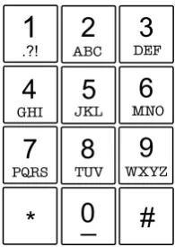
The 12-key input is the most common keypad lay-out on cellular telephones. It divides the alpha-bet into eight lists of characters and each list is mapped onto one key as shown in Figure 1. Since three or four characters are assigned to a key, a single key press is ambiguous.

Figure 1: Standard 12-button keypad layout (ISO 9995-8).

1.1 Multi-tap

Multi-tap is an elementary method to disam-biguate input for a 12-button keypad. Each charac-ter on a key is assigned an index that corresponds to its visual position, e.g. ‘A’, 1, ‘B’, 2, and ‘C’, 3 and each consecutive stroke – tap – on the same key increments the index. When the user wants to type a letter, s/he presses the corresponding key until the desired index is reached. The user then presses another key or waits a predefined time to verify that the correct letter is selected. The key sequence 8-4-4-3-3, for example, leads to the word the.

Multi-tap is easy to implement and no dictio-nary is needed. At the same time, it is slow and tedious for the user, notably when two consecutive characters are placed on the same key.

1.2 Single Tap with Predictive Text

Single tap with predictive text requires only one key press to enter a character. Given a keystroke sequence, the system proposes words using a dic-tionary or language modeling techniques.

Dictionary-based techniques search the words matching the key sequence in a list that is stored by the system (Haestrup, 2001). While some

keystroke sequences produce a unique word, oth-ers are ambiguous and the system returns a list with all the candidates. The key sequence 8-4-3, for example, corresponds to at least three possi-ble words: the,tie, andvie. The list of candidates is then sorted according to certain criteria, such as the word or character frequencies. If the word does not exist in the dictionary, the user has to fall back to multi-tap to enter it. The T91_commercial

product is an example of a dictionary-based sys-tem (Grover et al., 1998).

LetterWise (MacKenzie et al., 2001) is a tech-nique that uses letter trigrams and their frequen-cies to predict the next character. For example, pressing the key 3 after the letter bigram ‘th’ will select ‘e’, because the trigram ‘the’ is far more fre-quent than ‘thd’ or ‘thf’ in English. When the sys-tem proposes a wrong letter, the user can access the next most likely one by pressing a next-key. LetterWise does not need a dictionary and has a

KSP Cof 1.1500 (MacKenzie, 2002).

1.3 Modeling the Context

Language modeling can extend the context from letter sequences to wordn-grams. In this case, the

system is not restricted to the disambiguation or the prediction of the typed characters. It can com-plete words and even predict phrases. HMS (Has-selgren et al., 2003) is an example of this that uses word bigrams in Swedish. It reports a KSP C

ranging from 0.8807 to 1.0108, depending on the type of text. eZiText2_{is a commercial example of}

a word and phrase completion system. However, having a large lexicon of bigrams still exceeds the memory capacity of many mobile devices.

Some systems use a combination of syntac-tic and semansyntac-tic information to model the con-text. Gong et al. (2008) is a recent example that uses word frequencies, a part-of-speech language model, and a semantic relatedness metric. The part-of-speech language model acts as a lexical

n-gram language model, but occupies much less

memory since the vocabulary is restricted to the part-of-speech tagset. The semantic relatedness, modified from Li and Hirst (2005), is defined as the conditional probability of two stems appearing in the same context (the same sentence):

1_www.t9.com

2_{www.zicorp.com/ezitext.htm}

SemR(w1|w2) =

C(stem(w1), stem(w2))

C(w2)

.

The three components are combined linearly and their coefficients are adjusted using a devel-opment set. Setting 1 as the limit of the KSP C

figure, Gong et al. (2008) reported an error reduc-tion over the word frequency baseline of 4.6% for the semantic model, 12.6% for the part-of-speech language model, and 15.8% for the combination of both.

1.4 Syntax in Predictive Text

Beyond part-of-speech language modeling, there are few examples of systems using syntax in pre-dictive text entry. Matiasek et al. (2002) describes a predictive text environment aimed at disabled persons, which originally relied on language mod-els. Gustavii and Pettersson (2003) added a syn-tactic component to it based on grammar rules. The rules corresponded to common grammatical errors and were used to rerank the list of candidate words. The evaluation results were disappointing and the syntactic component was not added be-cause of the large overhead it introduced (Mati-asek, 2006).

In the same vein, Sundarkantham and Shalinie (2007) used grammar rules to discard infeasible grammatical constructions. The authors evaluated their system by giving it an incomplete sentence and seeing how often the system correctly guessed the next word (Shannon, 1951). They achieved better results than previously reported, although their system has not been used in the context of predictive text entry for mobile devices.

2 Predictive Text Entry Using Syntax We propose a new technique that makes use of a syntactic component to model the word context and improve theKSP Cfigure. It builds on Gong

et al. (2008)’s system and combines a dependency grammar model with word frequencies, a part-of-speech language model, and the semantic related-ness defined in Sect. 1.3. As far as we are aware, no predictive text entry system has yet used a data-driven syntactic model of the context.

2.1 Reranking Candidate Words

The system consists of two components. The first one disambiguates the typed characters using a dictionary and produces a list of candidate words. The second component reranks the candidate list. Although the techniques we describe could be ap-plied to word completion, we set aside this aspect in this paper.

More formally, we frame text input as a se-quence of keystrokes, ksi _{= ks}i

1. . . ksin, to en-ter a desired word, wi. The words matching the key sequence in the system dictionary form an ordered set of alternatives, match(ksi) = {cw0, . . . , cwm}, where it takeskextra keystrokes to reach candidate cwk. Using our example in Sect. 1.2, a lexical ordering would yield

match(8−4−3) = {the, tie, vie}, where two extra keystrokes are needed to reachvie.

We assign each candidate word w member of

match(ksi)a score

Score(w_|Context) =X

s∈S

λs·s(w|Context),

to rerank (sort) the prediction list, where s is a

scoring function from a setS, λs, the weight of

s, andScore(w_|Context), the total score ofwin

the current context.

In this framework, optimizing predictive text entry is the task of finding the scoring functions,

s, and the weights,λs, so that they minimizekon average.

As scoring functions, we considered lexical lan-guage models in the form of unigrams and bi-grams, sLM1 and sLM2, a part-of-speech model

using sequences of part-of-speech tags of a length of up to five tags, sP OS, and a semantic affin-ity,sSemA, derived from the semantic relatedness. In addition, we introduce a syntactic component in the form of a data-driven dependency syntax,

sDepSynso that the complete scoring set consists of

S =_{sLM1, sLM2, sSemA, sP OS, sDepSyn}.

2.2 Language and Part-of-Speech Models

The language model score is the probability of a candidate wordw, knowing the sequence entered

so far,w1, . . . , wi:

P(w_|w1, w2, . . . , wi).

We approximate it using unigrams, sLM1(w) =

P(w), or bigrams,sLM2(w) = P(w|wi) that we

derive from a corpus using the maximum like-lihood estimate. To cope with sparse data, we used a deleted interpolation so that sLM2(w) =

β1P(w|wi) +β2P(w), where we adjusted the

val-ues ofβ1andβ2on a development corpus.

In practice, it is impossible to maintain a large list of bigrams on cellular telephones as it would exceed the available memory of most devices. In our experiments, thesLM2score serves as an

indi-cator of an upper-limit performance, whilesLM1

serves as a baseline, as it is used in commercial dictionary-based products.

Part-of-speech models offer an interesting alter-native to lexical models as the number of parts of speech does not exceed 100 tags in most lan-guages. The possible number of bigrams is then at most 10,000 and much less in practice. We defined the part-of-speech model score,sP OSas

P(t|t1, t2, . . . , ti),

whereti is the part of speech ofwiandt, the part of speech of the candidate word w. We used a

5-gram approximation of this probability with a simple back-off model:

sP OS=           

P(t_|ti−3, . . . , ti) ifC(ti−3, ..., ti)6= 0

P(t|ti−2, . . . , ti) ifC(ti−2, ..., ti)6= 0 ...

P(t), otherwise

We used the Granska tagger (Carlberger and Kann, 1999) to carry out the part-of-speech anno-tation of the word sequence.

3 Semantic Affinity

Because of their arbitrary length, language mod-els miss possible relations between words that are semantically connected in a sentence but within a distance greater than one, two, or three words apart, the practical length of mostn-grams

mod-els. Li and Hirst (2005) introduced the semantic relatedness between two words to measure such relations within a sentence. They defined it as

SemR(wi, wj) =

C(wi, wj)

C(wi)C(wj)

,

whereC(wi, wj)is the number of times the words

andC(wi)is the count of wordwi in the corpus. The relation is symmetrical, i.e.

C(wi, wj) =C(wj, wi).

The estimated semantic affinity of a wordwis defined as:

SemA(w_|H) = X

wj∈H

SemR(w, wj),

whereHis the context of the wordw. In our case, Hconsists of words to the left of the current word.

Gong et al. (2008) used a similar model in a pre-dictive text application with a slight modification to theSemRfunction:

SemR(wi, wj) =

C(stem(wi), stem(wj))

C(stem(wj))

,

where the stem(w) function removes suffixes

from words. We refined this model further and we replaced the stemming function with a real lemma-tization.

4 Dependency Parsing

Dependency syntax (Tesnière, 1966) has attracted a considerable interest in the recent years, spurred by the availability of data-driven parsers as well as annotated data in multiple languages includ-ing Arabic, Chinese, Czech, English, German, Japanese, Portuguese, or Spanish (Buchholz and Marsi, 2006; Nivre et al., 2007). We used this syntactic formalism because of its availability in many languages.

4.1 Parser Implementation

There are two main classes of data-driven de-pendency parsers: graph-based (McDonald and Pereira, 2006) and transition-based (Nivre, 2003). We selected Nivre’s parser because of its imple-mentation simplicity, small memory footprint, and linear time complexity. Parsing is always achieved in at most2n₋1actions, wherenis the length of the sentence. Both types of parser can be com-bined, see Zhang and Clark (2008) for a discus-sion.

Nivre’s parser is an extension to the shift– reduce algorithm that creates a projective and acyclic graph. It uses a stack, a list of input words, and builds a set of arcs representing the graph of dependencies. The parser uses two operations in addition to shift and reduce, left-arc and right-arc:

• Shif t pushes the next input word onto the

stack.

• Reduce pops the top of the stack with the

condition that the corresponding word has a head.

• Lef tArc adds an arc from the next input

word to the top of the stack and pops it.

• RightArc adds an arc from the top of the

stack to the next input word and pushes the input word on the stack.

Table 1 shows the start and final parser states as well as the four transitions and their conditions and Algorithm 1 describes the parsing algorithm.

4.2 Features

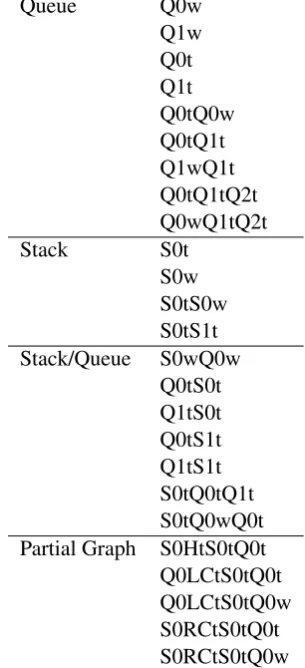
At each step of the parsing procedure, the parser turns to a guide to decide on which transition to apply among the set {Lef tArc, RightArc, Shif t, Reduce}. We implemented this guide

as a four-class classifier that uses features it ex-tracts from the parser state. The features consist of words and their parts of speech in the stack, in the queue, and in the partial graph resulting from what has been parsed so far. The classifier is based on a linear logistic regression function that evalu-ates the transition probabilities from the features and predicts the next one.

In the learning phase, we extracted a data set of feature vectors using the gold-standard parsing procedure (Algorithm 2) that we applied to Tal-banken corpus of Swedish text (Einarsson, 1976; Nilsson et al., 2005). Each vector being labeled with one of the four possible transitions. We trained the classifiers using the LIBLINEAR im-plementation (Fan et al., 2008) of logistic regres-sion.

However, classes are not always separable us-ing linear classifiers. We combined sus-ingle features as pairs or triples. This emulates to some extent quadratic kernels used in support vector machines, while preserving the speed of the linear models. Table 2 shows the complete feature set to predict the transitions. A feature is defined by

• A source:Sfor stack andQfor the queue;

Name Action Condition Initialization hnil, W,_∅i

Termination hS, nil, A_i

Lef tArc hn|S, n0|Q, Ai → hS, n0|Q, A∪ {hn0, ni}i ¬∃n00,hn, n00i ∈A RightArc hn|S, n0|Q, Ai → hn0|n|S, Q, A∪ hn, n0ii ¬∃n00,hn0, n00i ∈A Reduce _hn_|S, Q, A_{i → h}S, Q, A_{i ∃}n0,_hn, n0_{i ∈}A Shif t hS, n|Q, Ai → hn|S, Q, Ai

Table 1: Parser transitions. W is the original input sentence,Ais the dependency graph,S is the stack,

andQis the queue. The triplet_hS, Q, A_irepresents the parser state. n,n0, andn00are lexical tokens. The

pairhn0, nirepresents an arc from the headn0 to the dependentn.

• Possible applications of the function head,H, leftmost child,LC, or righmost child,RC;

• The value: word, w, or POS tag, t, at the

specified position.

Queue Q0w

Q1w Q0t Q1t Q0tQ0w Q0tQ1t Q1wQ1t Q0tQ1tQ2t Q0wQ1tQ2t

Stack S0t

S0w S0tS0w S0tS1t Stack/Queue S0wQ0w

Q0tS0t Q1tS0t Q0tS1t Q1tS1t S0tQ0tQ1t S0tQ0wQ0t Partial Graph S0HtS0tQ0t

Q0LCtS0tQ0t Q0LCtS0tQ0w S0RCtS0tQ0t S0RCtS0tQ0w

Table 2: Feature model for predicting parser ac-tions with combined features.

4.3 Calculating Graph Probabilities

Nivre (2006) showed that every terminating tran-sition sequence Am

1 = (a1, ..., am) applied to

a sentence Wn

1 = (w1, ..., wn) defines exactly one parse tree G. We approximated the

prob-ability P(G_|W₁n) of a dependency graph G as P(Am

1 |W1n) and we estimated the probability of

Gas the product of the transition probabilities, so

that

PP arse(G|W1n) = P(Am1 |W1n)

= Qm_k=1P(ak|Ak1−1, W

φ(k−1) 1 ),

where ak is member of the set {Lef tArc,

RightArc, Shif t, Reduce} and φ(k)

corre-sponds to the index of the current word at tran-sitionk.

We finally approximated the term

Ak₁−1, W₁φ(k−1) to the feature set and com-puted probability estimates using the logistic regression output.

4.4 Beam Search

We extended Nivre’s parser with a beam search to mitigate error propagation that occurs with a de-terministic parser (Johansson and Nugues, 2006). We maintainedN parser states in parallel and we

applied all the possible transitions to each state. We scored each transition action and we ranked the states with the product of the action’s proba-bilities leading to this state. Algorithm 3 outlines beam search with a diameter ofN.

4.5 Evaluation

We evaluated our dependency parser separately from the rest of the application and Table 3 shows the results. We optimized our parameter selection for the unlabeled attachment score (UAS). This explains the relatively high difference with the la-beled attachment score (LAS): about –8.6.

Table 3 also shows the highest scores ob-tained on the same Talbanken corpus of Swedish text (Einarsson, 1976; Nilsson et al., 2005) in the CoNLL-X evaluation (Buchholz and Marsi, 2006): 89.58 for unlabeled attachments (Corston-Oliver and Aue, 2006) and 84.58 for labeled at-tachments (Nivre et al., 2006). CoNLL-X systems were optimized for the LAS category.

The figures we reached were about 1.10% be-low those reported in CONLL-X for the UAS cat-egory. However our results are not directly compa-rable as the parsers or the classifiers in CONLL-X have either a higher complexity or are more time-consuming. We chose linear classifiers over kernel machines as it was essential to our application to run on mobile devices with limited resources in both CPU power and memory size.

This paper CONLL-X Beam width LAS UAS LAS UAS

1 79.45 88.05 84.58 89.54 2 79.76 88.41

4 79.75 88.40 8 79.77 88.41 16 79.78 88.42 32 79.77 88.41 64 79.79 88.44

Table 3: Parse results on the Swedish Talbanken corpus obtained for this paper as well as the best reported results in CONLL-X on the same corpus (Buchholz and Marsi, 2006).

5 Dependencies to Predict the Next Word We built a syntactic score to measure the grammat-ical relevance of a candidate wordwin the current

context, that is the word sequence so farw1, ..., wi. We defined it as the weighted sum of three terms: the score of the partial graph resulting from the analysis of the words to the left of the candidate word and the scores of the link fromwto its head, h(w), using their lexical forms and their parts of

speech:

sDepSyn(w) =λ1PP arse(G(w)|w1, ..., wi, w)+

λ2PLink(w, h(w))+

λ3PLink(P OS(w), P OS(h(w))),

whereG(w) is the partial graph representing the

word sequencew1, ..., wi, w. ThePLink terms are intended to give an extra-weight to the probabil-ity of an association between the predicted word and a possible head to the left of it. They hint at the strength of the ties between wand the words

before it.

We used the transition probabilities described in Sect. 4.3 to compute the score of the partial graph, yielding

PP arse(G(w)|w1, ..., wi, w) = j Y

k=1

P(ak),

where a1, ..., aj is the sequence of transition ac-tions producingG(w) andP(ak), the probability output of transitionkgiven by the logistic

regres-sion engine.

The last two terms PLink(w, h(w)) and

PLink(P OS(w), P OS(h(w))) are computed from counts in the training corpus using maxi-mum likelihood estimates:

PLink(w, h(w)) =

C(Link(w, h(w)) + 1

P

wl∈P WC(Link(wl, h(wl)))

+_|P W_|

and

PLink(P OS(w), P OS(h(w))) =

C(Link(P OS(w), P OS(h(w)))) + 1

P

wl∈P WC(Link(P OS(wl), h(P OS(wl))))

+_|P W_|,

whereP W =match(ksi), is the set of predicted

words for the current key sequence.

If the current word whas not been assigned a head yet, we defaulth(w)to the root of the graph

andP OS(h(w))to theROOT value.

6 Experiments and Results

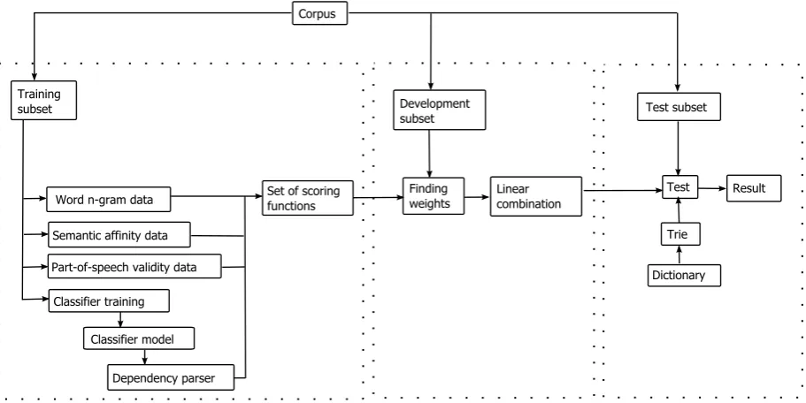
6.1 Experimental Setup

tuning, and testing. Ideally, we would have trained the classifiers on a corpus matching a text entry application. However, as there is no large available SMS corpus in Swedish, we used the Stockholm-Umeå corpus (SUC) (Ejerhed and Källgren, 1997). SUC is balanced and the largest available POS-tagged corpus in Swedish with more than 1 million words.

We parsed the corpus and we divided it ran-domly into a training set (80%), a development set (10%), and a test set (10%). The training set was used to gather statistics on word n-grams, POS n-grams, collocations, lemma frequencies,

depen-dent/head relations. We discarded hapaxes: rela-tions and sequences occurring only once. We used lemmas instead of stems in the semantic related-ness score, SemR, because stemming is less

ap-propriate in Swedish than in English.

We used the development set to find optimal weights for the scoring functions, resulting in the lowest KSPC. We ran an exhaustive search using all possible linear combinations with increments of 0.1, except for two functions, where this was too coarse. We used 0.01 then.

We applied the resulting linear combinations of scoring functions to the test set. We first compared the frequency-based disambiguation acting as a baseline to linear combinations involving or not involving syntax, but always excluding bigrams. Table 4 shows the most significant combinations. We then compared a set of other combinations with the bigram model. They are shown in Ta-ble 6.

6.2 Metrics

We redefined the KSPC metric of MacKenzie (2002), since the number of characters needed to input a word is now dependent on the word’s left context in the sentence. LetS = (w1, . . . , wn)∈

Lbe a sentence in the test corpus. The KSPC for

the test corpus then becomes

KSP C=

P S∈L

P

w∈SKS(w|LContext(w, S)) P

S∈L P

w∈SChars(w)

where KS(w_|LContext) is the number of key

strokes needed to enter a word in a given context,

LContext(w, S)is the left context ofwinS, and Chars(w)is the number of characters inw.

Another performance measure is the disam-biguation accuracy (DA), which is the percentage of words that are correctly disambiguated after all

the keys have been pressed

DA=

X

S∈L X

w∈S

P redHit(w|LContext(w, S))

#w ,

where P redHit(w_|Context) = 1 if w is the

top prediction and 0 otherwise, and #w, the

to-tal number of words inL. A good DA means that

the user can more often simply accept the default proposed word instead of navigating the prediction list for the desired word.

As scoring tokens, we chose to keep the ones that actually have the ability to differentiate the models, i.e. we did not count the KSPC and DA for words that were not in the dictionary. Neither did we count white spaces, nor the punctuation marks.

All our measures are without word or phrase completion. This means that the lower-limit fig-ure forKSP Cis 1.

6.3 Results

As all the KSPC figures are close to 1, we com-puted the error reduction rate (ERR), i.e. the re-duction in the number of extra keystrokes needed beyond one. We carried out all the optimizations considering KSPC, but we can observe that KSPC ERR and DA ERR strongly correlate.

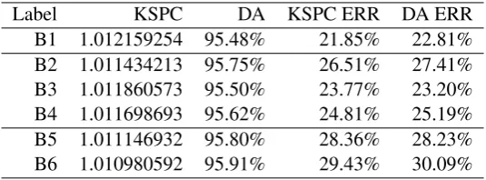
Table 5 shows the results with scoring func-tions using the word frequencies. The columns include KSPC and DA together with KSPC ERR and DA ERR compared with the baseline. Table 7 shows the respective results when using a bigram-based disambiguation instead of just frequency. The ERR is still compared to the word frequency baseline but attention should also be drawn on the relative increases: how much the new models can improve bigram-based disambiguation.

7 Discussion

We can observe from the results that a model based on dependency grammars improves the prediction considerably. TheDepSynmodel is actually the

most effective one when applied together with the frequency counts. Furthermore, the improvements from theP OS, SemA, andDepSyn model are

almost disjunct, as the combined model improve-ment matches the sum of their respective individ-ual contributions.

The 4.2% ERR observed when adding the

Figure 2: System architecture, where the set of scoring functions isS =_{sLM, sSemA, sP OS, sDepSyn} and the linear combination is=X

s∈S

λs·s(w).

Gong et al. (2008), where a 4.6% ERR was found. On the other hand, the P OS model only con-tributed 4.7% ERR in our case, whereas Gong et al. (2008) observed 12.6%. One possible expla-nation for this is that they clustered related POS tags into 19 groups reducing the sparseness prob-lem. By performing this grouping, we can effec-tively ignore morphological and lexical features that have no relevance, when deciding which word should come next. Other possible explanations in-clude that our backoff model is not well suited for this problem or that the POS sequences are not an applicable model for Swedish.

The bigram language model has the largest im-pact on the performance. The ERR for bigrams alone is higher than all the other models com-bined. Still, the other models have the ability to contribute on top of the bigram model. For exam-ple, the P OSmodel increases the ERR by about

5% both when using bigram- and frequency-based disambiguation, suggesting that this information is not captured by the bigrams. On the other hand,

DepSynincreases the ERR by a more modest 3%

when using bigrams instead of 7% with word fre-quencies. This is likely due to the fact that about half of the dependency links only stretch to the next preceding or succeeding word in the corpus.

The most effective combination of models are the bigrams together with the POS sequence and

the dependency structure, both embedding syntac-tic information. With this combination, we were able to reduce the number of erroneous disam-biguations as well as extra keystrokes by almost one third.

8 Further Work

SMS texting, which is the target of our system, is more verbal than the genres gathered in the Stockholm-Umeå corpus. The language models of a final application would then change consid-erably from the ones we extracted from the SUC. A further work would be to collect a SMS corpus and replicate the experiments: retrain the models and obtain the corresponding performance figures. Moreover, we carried out our implementation and simulations on desktop computers. TheP OS

be needed to prove an implementability on mobile devices.

Finally, a user might perceive subtle differences in the presentation of the words compared with that of popular commercial products. Gutowitz (2003) noted the reluctance to single-tap input methods because of their “unpredictable” behav-ior. Introducing syntax-based disambiguation could increase this perception. A next step would be to carry out usability studies and assess this el-ement.

References

Sabine Buchholz and Erwin Marsi. 2006. CoNLL-X shared task on multilingual dependency parsing. In Proceedings of the Tenth Conference on Com-putational Natural Language Learning (CoNLL-X), pages 149–164, New York City.

Johan Carlberger and Viggo Kann. 1999.

Implement-ing an efficient part-of-speech tagger. Software –

Practice and Experience, 29(2):815–832.

Simon Corston-Oliver and Anthony Aue. 2006. De-pendency parsing with reference to slovene, spanish

and swedish. InProceedings of the Tenth

Confer-ence on Computational Natural Language Learning (CoNLL-X), pages 196–200, New York City, June.

Jan Einarsson. 1976. Talbankens skriftspråkskonkor-dans. Technical report, Lund University, Institutio-nen för nordiska språk, Lund.

Eva Ejerhed and Gunnel Källgren. 1997. Stockholm Umeå Corpus version 1.0, SUC 1.0.

Rong-En Fan, Kai-Wei Chang, Cho-Jui Hsieh, Xiang-Rui Wang, and Chih-Jen Lin. 2008. LIBLINEAR: A library for large linear classification. Journal of Machine Learning Research, 9:1871–1874.

Jun Gong, Peter Tarasewich, and I. Scott MacKenzie. 2008. Improved word list ordering for text entry on

ambiguous keypads. InNordiCHI ’08: Proceedings

of the 5th Nordic conference on Human-computer interaction, pages 152–161, Lund, Sweden.

Dale L. Grover, Martin T. King, and Clifford A. Kush-ler. 1998. Reduced keyboard disambiguating com-puter. U.S. Patent no. 5,818,437.

Ebba Gustavii and Eva Pettersson. 2003. A Swedish grammar for word prediction. Technical report, De-partment of Linguistics, Uppsala University.

Howard Gutowitz. 2003. Barriers to adoption of dictionary-based text-entry methods; a field study. InProceedings of the Workshop on Language Mod-eling for Text Entry Systems (EACL 2003), pages 33– 41, Budapest.

Jan Haestrup. 2001. Communication terminal hav-ing a predictive editor application. U.S. Patent no. 6,223,059.

Jon Hasselgren, Erik Montnemery, Pierre Nugues, and Markus Svensson. 2003. HMS: A predictive text

entry method using bigrams. In Proceedings of

the Workshop on Language Modeling for Text Entry Methods (EACL 2003), pages 43–49, Budapest.

Richard Johansson and Pierre Nugues. 2006.

In-vestigating multilingual dependency parsing. In

Proceedings of the Tenth Conference on Compu-tational Natural Language Learning (CONLL-X), pages 206–210, New York.

Richard Johansson and Pierre Nugues. 2007. Incre-mental dependency parsing using online learning. In Proceedings of the CoNLL Shared Task Session of EMNLP-CoNLL, pages 1134–1138, Prague, June 28-30.

Jianhua Li and Graeme Hirst. 2005. Semantic

knowl-edge in word completion. InAssets ’05:

Proceed-ings of the 7th international ACM SIGACCESS con-ference on Computers and accessibility, pages 121– 128, Baltimore.

I. Scott MacKenzie, Hedy Kober, Derek Smith, Terry Jones, and Eugene Skepner. 2001. LetterWise: Prefix-based disambiguation for mobile text input. In14th Annual ACM Symposium on User Interface Software and Technology, Orlando, Florida.

I. Scott MacKenzie. 2002. KSPC (keystrokes per char-acter) as a characteristic of text entry techniques. In

Proceedings of the Fourth International Symposium on Human Computer Interaction with Mobile De-vices, pages 195–210, Heidelberg, Germany.

Johannes Matiasek, Marco Baroni, and Harald Trost. 2002. FASTY – A multi-lingual approach to text

prediction. In ICCHP ’02: Proceedings of the

8th International Conference on Computers Helping People with Special Needs, pages 243–250, London.

Johannes Matiasek. 2006. The language component of the FASTY predictive typing system. In Karin Harbusch, Kari-Jouko Raiha, and Kumiko Tanaka-Ishii, editors,Efficient Text Entry, number 05382 in Dagstuhl Seminar Proceedings, Dagstuhl, Germany.

Ryan McDonald and Fernando Pereira. 2006. Online learning of approximate dependency parsing algo-rithms. InProceedings of the 11th Conference of the European Chapter of the Association for Computa-tional Linguistics (EACL), pages 81–88, Trento.

Jens Nilsson, Johan Hall, and Joakim Nivre. 2005. MAMBA meets TIGER: Reconstructing a Swedish

treebank from antiquity. In Proceedings of the

Joakim Nivre, Johan Hall, Jens Nilsson, Gülsen Eryigit, and Svetoslav Marinov. 2006. Labeled pseudo-projective dependency parsing with support

vector machines. InProceedings of the Tenth

Con-ference on Computational Natural Language Learn-ing (CoNLL-X), pages 221–225, June.

Joakim Nivre, Johan Hall, Sandra Kübler, Ryan Mc-Donald, Jens Nilsson, Sebastian Riedel, and Deniz Yuret. 2007. The CoNLL 2007 shared task on

de-pendency parsing. In Proceedings of the CoNLL

Shared Task Session of EMNLP-CoNLL 2007, pages 915–932, Prague.

Joakim Nivre. 2003. An efficient algorithm for

pro-jective dependency parsing. In Proceedings of the

8th International Workshop on Parsing Technologies (IWPT), pages 149–160, Nancy.

Joakim Nivre. 2006. Inductive Dependency Parsing.

Springer, Dordrecht, The Netherlands.

Claude Elwood Shannon. 1951. Prediction and en-tropy of printed English. The Bell System Technical Journal, pages 50–64, January.

K. Sundarkantham and S. Mercy Shalinie. 2007. Word predictor using natural language grammar induction

technique. Journal of Theoretical and Applied

In-formation Technology, 3:1–8.

Lucien Tesnière. 1966. Éléments de syntaxe

struc-turale. Klincksieck, Paris, 2e edition.

Yue Zhang and Stephen Clark. 2008. A tale of two parsers: Investigating and combining graph-based and transition-graph-based dependency parsing

us-ing beam-search. InProceedings of the 2008

Algorithm 1Nivre’s algorithm.

1: Queue⇐W

2: Stack_⇐nil

3: while_¬Queue.isEmpty()do

4: f eatures⇐ExtractF eatures()

5: action_⇐guide.P redict(f eatures)

6: if action=RightArc∧canRightArc() then

7: RightArc()

8: else if action=Lef tArc_∧canLef tArc() then

9: Lef tArc

10: else if action=Reduce∧canReduce() then

11: Reduce()

12: else 13: Shif t()

14: end if 15: end while 16: return(A)

Algorithm 2Reference parsing.

1: Queue_⇐W

2: Stack⇐nil

3: while_¬Queue.isEmpty()do

4: x_⇐ExtractF eatures()

5: if _hStack.peek(), Queue.get(0)i ∈A∧canRightArc()then

6: t⇐RightArc

7: else if _hQueue.get(0), Stack.peek()_{i ∈}A_∧canLef tArc()then

8: t⇐Lef tArc

9: else if∃w∈Stack:hw, Queue.get(0)i ∈A∨ hQueue.get(0), wi ∈A)∧canReduce()then

10: t_⇐Reduce

11: else

12: t⇐Shif t

13: end if

14: store training examplehx, t_i

15: end while

Algorithm 3Beam parse.

1: Agenda.add(InititalP arserState)

2: while¬donedo

3: forparserState_∈Agendado

4: Output.add(parserState.doLef tArc())

5: Output.add(parserState.doRightArc())

6: Output.add(parserState.doReduce())

7: Output.add(parserState.doShif t())

8: end for 9: Sort(Output)

10: Clear(Agenda)

11: TakeN best parse trees fromOutputand put inAgenda.

12: end while

Configuration Scoring model DepSynweights

F1 baseline 1×LM1(Word frequencies) –

F2 0.9_×LM1 + 0.1_×P OS –

F3 0.7_×LM1 + 0.3_×SemA –

F4 0.6×LM1 + 0.4×DepSyn (0.3, 0.7, 0.0)

F5 0.6×LM1 + 0.1×P OS+ 0.3×DepSyn (0.0 1.0 0.0)

F6 0.5_×LM1 + 0.2_×SemA+ 0.3_×DepSyn (0.2 0.7 0.1)

F7 0.4×LM1 + 0.1×P OS+ 0.3×DepSyn+ 0.2×SemA (0.2, 0.8, 0.0)

Table 4: The different combinations of scoring models using frequency-based disambiguation as a base-line. TheDepSynweight triples corresponds to(λ1, λ2, λ3)in Sect. 5.

Configuration KSPC DA KSPC ERR DA ERR

F1 1.015559 94.15% 0.00% 0.00%

F2 1.014829 94.31% 4.69% 2.72%

F3 1.014902 94.36% 4.22% 3.62%

F4 1.014462 94.56% 7.05% 7.04%

F5 1.013625 94.75% 12.43% 10.28%

F6 1.014159 94.62% 9.00% 8.10%

F7 1.013438 94.86% 13.63% 12.16%

Table 5: Results for the disambiguation based on word frequencies together with the semantic and syn-tactic models.

Configuration Scoring model Bigram weights DepSynweights

B1 1×LM2(Bigram frequencies) (0.9, 0.1) –

B2 0.9_×LM2 + 0.1_×P OS (0.8, 0.2) –

B3 0.95×LM2 + 0.05×SemA (0.8, 0.2) –

B4 0.9_×LM2 + 0.1_×DepSyn (0.8, 0.2) (0.2, 0.8, 0.0)

B5 0.8_×LM2 + 0.1_×P OS+ 0.1_×SemA (0.8, 0.2) –

B6 0.81_×LM2 + 0.08_×P OS+ 0.11_×DepSyn (0.8, 0.2) (0.2, 0.8, 0.0)

Table 6: The different combinations of scoring models using bigram-based disambiguation as baseline. In addition to theDepSynweights, this table also shows the language model interpolation weights,β1

andβ2described in Sect. 2.2.

Label KSPC DA KSPC ERR DA ERR B1 1.012159254 95.48% 21.85% 22.81% B2 1.011434213 95.75% 26.51% 27.41% B3 1.011860573 95.50% 23.77% 23.20% B4 1.011698693 95.62% 24.81% 25.19% B5 1.011146932 95.80% 28.36% 28.23% B6 1.010980592 95.91% 29.43% 30.09%