Volume 2, No. 5, Sept-Oct 2011
International Journal of Advanced Research in Computer Science
RESEARCH PAPER
Available Online at www.ijarcs.info
ISSN No. 0976-5697
Comparative Analysis Of BNP Scheduling Algortihms
Ravreet Kaur
Department of Computer Sci. & Engg. Guru Nanak Dev University
Amritsar, Punjab, India [email protected]
Abstract: Parallel Computing is the procedure of creating an environment where requirement of the job is equated with the available resources in system. Multiprocessor task scheduling is most important and very crucial issue in design of homogeneous parallel systems. This paper covers the study of scheduling algorithms related to Bounded Number of Processors (BNP) class of multiprocessor scheduling algorithm represented by a Directed Acyclic graph (DAG). An attempt has been made to evaluate their performance on basis of Processor Utilization, SpeedUp and Scheduled Length Ratio (SLR). Analysis of the performance has proved Dynamic Level Scheduling (DLS) as a better algorithm in homogeneous environment.
Keywords: Directed Acyclic Graph (DAG), Dynamic Level Scheduling (DLS), Homogeneous Environment, Multiprocessor Scheduling algorithm, Parallel Computing, Multiprocessor task scheduling, Processor Utilization, Scheduled Length Ratio (SLR), SpeedUp.
I. INTRODUCTION
The field of parallel task scheduling is one of the most advanced and rapidly evolving fields in computer sciences. Parallel computing is expected to bring a break-through in the increase of computing speed and efficiency. This calls for appropriate scheduling strategies controlling access to such resources as well as scheduling strategies controlling execution of the parallel application modules. The scheduling problem deals with the optimal assignments of a set of tasks onto parallel resources and orders their execution to achieve optimal objective function.
This paper employs the generic DAG model and discusses its variations and suitability to different situations. Further the basic strategies of scheduling algorithms i.e. APN, UNC, TDB and BNP algorithms are discussed. The BNP class of algorithms are discussed in detail giving their comparative analysis.
A. The DAG Model:
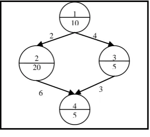
The DAG [1][2] is a generic model of a parallel program consisting of a set of processes dependent on each other as shown in Figure 1. Each process is an indivisible unit of execution, expressed by a node. A node has one or more inputs and can have one or more outputs to various nodes. Node is triggered to execute once all its inputs are available, resulting in its outputs. In this model, a set of n nodes {n1,
n2, n3…nn} are connected by a set of e directed edges, which
are represented by (ni, nj) where ni is called the Parent node
and nj is called the Child node. A node without parent is
called an Entry node and a node without child is called an
Exit node.
The weight of a node denoted by w (ni), represents the
process execution time of a process. Since each edge corresponds to a message transfer from one process to another, the weight of an edge, denoted by c(ni, nj) , is equal
to the message transmission time from node ni to nj. Thus,
c(ni, nj) becomes zero when ni and nj are scheduled to the
same processor because intraprocessor communication time is negligible compared with the interprocessor
communication time. The node and edge weights are usually obtained by estimations.
Figure 1. Directed Acyclic Graph
II. LITERATURESURVEY
Ishfaq Ahmad, Yu-Kwong Kwok [1] evaluated and compared algorithms for scheduling and clustering. These algorithms allocate a parallel program represented by an edge-weighted directed acyclic graph (DAG), to a set of homogeneous processors, to minimize the completion time.
Yu-Kwong Kwok [2] [4] has categorized the algorithms in various sets like UNP, BNP, APN, TDB and have used various parameters like algorithm running time, the number of processors used, comparison with each other, number of best solutions attained etc. to evaluate the multiprocessor task scheduling algorithms. Thomas G. Price [3] has done an exact analysis of processor utilization using shortest-remaining-processing-time scheduling for systems with two jobs given and it is observed that the processor utilization is independent of the form of the processing time distribution. T. Hagras, J. Janeček [5] gave an idea of efficient task scheduling algorithms in homogenous environments, and also provided with an efficient scheduling techniques using list scheduling techniques in static and dynamic environment. J.K. Lenstra, A.H.G Rainnooy Kan [6]
surveyed all the recent algorithms for multiprocessor scheduling, presented the basic models of scheduling and
6 3
2 4
2 20
3 5
provided with the framework for presenting the results of these algorithms. Min-You Wu [7] showed that most of the parallel tasks which are represented by DAG are sequential.
Two efficient static task scheduling algorithms were discussed and their performance is evaluated on Intel Paragon machine. Arezou Mohammadi and Selim G. Akl [11] studied the characteristics and constraints of real-time tasks which should be scheduled to be executed. Analysis methods and the concept of optimality criteria, which leads to the design of appropriate scheduling algorithms, was also addressed. Also both the preemptive and non-preemptive static-priority based algorithms are also discussed. Guolong Lin, Rajmohan Rajaraman [13] studied multiprocessor scheduling in scenarios where there is uncertainty in the successful execution of jobs when assigned to processors.
They considered the problem of multiprocessor scheduling under uncertainty, in which there are given n unit-time jobs and m machines, a directed acyclic graph C giving the dependencies among the jobs, and for every job j and machine i, the probability Pij of the successful
completion of job j when scheduled on machine i in any given particular step. They found a schedule that minimizes the expected makespan, that is, the expected completion time of all the jobs. Bernard Chauvi`ere, Dominique Geniet, Ren´e Schott [14] proposed various algorithmic improvements for the multiprocessor scheduling problem.
Their simulation results showed that their methods produce solutions closer to optimality when the number of processors and/or the number of precedence constraints increases. Igor Grudenić [15] presented all the aspects of scheduler design such as system architectures, workload types, metrics, simulator tools and benchmarks. Overview of the existing scheduling techniques was also compared. S.V.
Sudha and K. Thanushkodi [16] presented the supple scheduling algorithm and fully implemented. Its results were compared with other scheduling algorithms like First Come First Serve, Gang Scheduling, Flexible Co Scheduling.
Thomas L. Casavant [18] presented taxonomy of approaches to the resource management problem in an attempt to provide a common terminology and classification mechanism necessary in addressing the problem. The resource management problem is defined as usage of general-purpose distributed computing system’s ability to provide a level of performance commensurate to the degree of multiplicity of resources present in the system. The taxonomy, while presented and discussed in terms of distributed scheduling, is also applicable to most types of resource management.
III. BASICCLASSESOFPARALLELSCHEDULING
Various parallel scheduling algorithms found in literature are presented below:
A. BNP Scheduling Algorithms:
BNP stands for Bounded Number of Processors [1] [2] [4]. These algorithms schedule the DAG to a bounded number of processors directly. The processors are assumed to be fully connected. Most BNP scheduling algorithms are based on the list scheduling technique.
B. APN Scheduling Algorithms:
The algorithms in this class take into account specific architectural features such as the number of processors as
well as their interconnection topology. These algorithms can schedule tasks on the processors and messages on the network communication links. Scheduling of messages may be dependent on the routing strategy used by the underlying network [1][2][4].
C. UNC Scheduling Algorithms:
UNC stands for Unbounded Number of Clusters [1] [2] [4]. These algorithms schedule the DAG to an unbounded number of clusters. The processors are assumed to be fully connected. The basic technique employed by UNC scheduling algorithms is called Clustering. At the beginning of the scheduling process, each node is considered as a cluster. In the subsequent steps, two clusters are merged if the merging reduces the completion time. This merging procedure continues until no cluster can be merged.
D. TDB Scheduling Algorithms:
The TDB stands for Task Duplication Based scheduling algorithms. The principle behind the TDB algorithms is to reduce the communication overhead by redundantly allocating some tasks to multiple processors [4].
IV. BNPSCEDULINGALGORITHMS
BNP stands for Bounded Number of Processors [1][2][4]. These algorithms schedule the DAG to a bounded number of processors directly. The processors are assumed to be fully connected. Most BNP scheduling algorithms are based on the list scheduling technique. List scheduling [9] is a class of scheduling heuristics in which the nodes are assigned priorities and placed in a list arranged in a descending order of priority. The node with a higher priority will be examined for scheduling before a node with a lower priority. If more than one node has the same priority, ties are broken using some method.
Two major attributes for assigning priority are the t-level (top level) and b-level (bottom level). The t-level of a node ni is the length of the longest path from an entry node to ni
node in the DAG excluding ni node. The length of a path is the sum of all the node weights and edge weights along the path. The t-level of ni is also known as ni’s Earliest start
time, denoted by T(ni), which is determined after ni is
scheduled to a processor.
The b-level of a node ni is the length of the longest path
from node ni, to an exit node. Only the weights of the nodes
are considered not the weights of the edges while measuring the b-level. The b-level of a node is bounded by the length of the critical path. A Critical Path (CP) of a DAG is a path from an entry node to an exit node, whose length is the maximum. The main examples of BNP algorithms are the HLFET (Highest Level First with Estimated Times) algorithm, the MCP (Modified Critical Path) algorithm, the DLS (Dynamic Level Scheduling) algorithm and the ETF (Earliest Task First) algorithm [1]. The summarized functioning of different algorithms under BNP is described in next sections.
A. HLFET Algorithm (Highest Level First with Estimated Time):
a. Calculate the Static Level of all the nodes in the DAG.
c. While not the end of the list do i. Remove node ni from the list.
ii. Compute the earliest start execution time of ni
for all the processor present in the system. iii. Map the node ni to the processor that has the
least earliest start execution time.
B. MCP Algorithm (Modified Critical Path):
a. Calculate the Latest Start Time (LST) of all the nodes in the DAG.
b. Insert all the nodes into a list and sort the list according to ascending order of Latest Start Time. c. While not the end of the list do
i. Remove the node from the list.
ii. Compute the earliest start execution time of ni
for all the processors present in the system. iii. Map the node ni to the processor that has the
least earliest start execution time.
C. ETF Algorithm (Earliest Task First):
a. Calculate the Static Level of each node in the DAG. b. In the beginning the ready node list contains only
ii. Select the node with earliest start time. If two or more nodes have same earliest execution start time values then the node with highest Static Level is selected.
iii. Map the selected node to the processor. iv. Add new ready nodes to the ready node list.
D. DLS Algorithm (Dynamic Level Scheduling):
a. Commute the Static Level of nodes in the DAG. b. In the beginning the ready node list contains only
the entry node.
c. While the ready node list is not empty do
i. Calculate the earliest start time of every node in the ready node list on each processor.
ii. Calculate the Dynamic Level of every node in the list.
iii. Select the node with largest Dynamic Level. iv. Schedule the node onto the processor.
v. Add new ready node in the ready node list. uniform distribution. The performance comparison is based on the following factors:
a. Processor Utilization: Processor utilization measure the percent of time for which the processor performed. Processor Utilization(%) = (Total execution time of scheduled tasks/Makespan) * 100
b. SpeedUp: Speed up is defined as the ratio of time taken by serial algorithm to perform work to the time taken by the parallel algorithm to perform the same work.
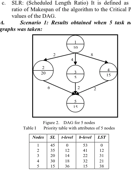
c. SLR: (Scheduled Length Ratio) It is defined as the ratio of Makespan of the algorithm to the Critical Path values of the DAG.
A. Scenario 1: Results obtained when 5 task node graphs was taken:
Figure 2. DAG for 5 nodes
Table I Priority table with attributes of 5 nodes
Nodes SL t-level b-level LST
Table II SLR, SpeedUp and Processor Utilization (P1, P2, and P3) of algorithms with 5 tasks
Algorithm SLR SpeedUp Processor Utilization
P1 P2 P3
HLFET 1.275 1.27451 58.82% 58.82% 9.80%
MCP 1.275 1.27451 58.82% 58.82% 9.80%
ETF 1.275 1.27451 58.82% 9.80% 58.82%
DLS 1.275 1.27451 58.82% 58.82% 9.80%
Figure 3. SLR and Speed Up with 5 nodes
B. Scenario 2: Results obtained when 10 task nodes graph was taken.:
Figure 5. DAG for 10 nodes
Table III Priority table with attributes of 10 nodes
Nodes SL t-level b-level LST
Table IV SLR, SpeedUp and Processor Utilization (P1, P2 and P3) of algorithms with 10 tasks
Algorithm SLR SpeedUp
Processor Utilization
Figure 6. SLR and SpeedUp with 10 nodes
Figure 7. Processor Utilization (P1, P2 and P3) with 10 nodes
C. Scenario 3: Results obtained when 15 task nodes graph was taken.:
Figure 8. DAG for 15 nodes
Table V Priority table with attributes of 15 nodes
Nodes SL t-level b-level LST
Table VI SLR, SpeedUp and Processor Utilization(P1, P2 and P3) of algorithms with 15 tasks
Algorithm SLR SpeedUp
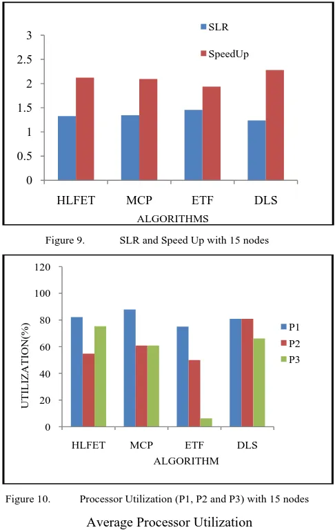
Figure 9. SLR and Speed Up with 15 nodes
Figure 10. Processor Utilization (P1, P2 and P3) with 15 nodes
Average Processor Utilization
Table VII Average processor Utilization comparison for BNP scheduling algorithms
Algorithms 5 Tasks 10 Tasks 15 Tasks
HLFET 42.48% 63.49% 70.78%
MCP 42.48% 65.57% 69.82%
ETF 42.48% 65.57% 43.75%
DLS 42.48% 65.57% 75.98%
Figure 11. Graph for average processor utilization comparison
Scheduled Length Ratio
Table VIIIScheduled Length Ratio comparison for BNP scheduling algorithms
Figure 12. Graph for scheduled length ratio comparison
Speed Up
Table IX SpeedUp comparison for BNP scheduling algorithms
Figure 13. Graph for speedup comparison
VI. CONCLUSIONANDFUTUREWORK
With Comparative analysis following result was attained:-
a. The Average Processor Utilization remained same for all algorithms with 5 tasks. MCP, ETF and DLS utilized processor efficiently than HLFET with 10 tasks. b. With 15 tasks, DLS proved to be better than other
algorithms and ETF showed almost 20% drop in utilization rate.
0 0.5 1 1.5 2 2.5 3
HLFET MCP ETF DLS
SLR
SpeedUp
ALGORITHMS
0 20 40 60 80 100 120
HLFET MCP ETF DLS
P1 P2 P3
ALGORITHM
UTI
LI
ZAT
ION(
%)
40 60 80
4 9 14
HLFET MCP
ETF
DLS
UTI
LI
ZAT
ION(
%)
TASKS
1.1 1.4 1.7 2
4 9 14
HLFE T
MCP
SLR
TASKS
1 1.4 1.8 2.2 2.6 3
4 9 14 19
HLFET
MCP
ETF
DLS
TASKS
SPEE
DUP
Algorithms 5 Tasks 10 Tasks 15 Tasks
HLFET 1.275 1.8 1.327273
MCP 1.275 1.742857 1.345455
ETF 1.275 1.742857 1.454545
DLS 1.275 1.742857 1.236364
Algorithms 5 Tasks 10 Tasks 15 Tasks
HLFET 1.27451 1.904762 2.123288
MCP 1.27451 1.967213 2.094595
ETF 1.27451 1.967213 1.9375
c. The SLR remained almost the same with 5 and 10 tasks within their respective tasks. With 15 tasks DLS was the one with lesser SLR.
d. Same is the case with Speed Up. With 5 and 10 tasks speed up of all algorithms was same within respective tasks. Again here DLS was the algorithm with higher Speed Up.
e. It can be concluded from the above results, that DLS is one of the efficient algorithms, considering the data gathered using the scenarios and the performance calculated from them.
f. This paper has a lot of future scope. Lots of work can be done considering more case scenarios:-
i. Heterogeneous environment can be considered, in which multiple processors having different configuration are used.
ii. Combination of both Homogenous and Heterogeneous can be considered.
iii. The numbers of tasks can be changed to create test case scenarios.
iv. More algorithms can be considered and their performance with other can be estimated.
VII.REFERENCES
[1] Ishfaq Ahmad and Yu-Kwong Kwok, “Performance Comparison of Algorithms for Static Scheduling of DAGs to Multiprocessors” in Second Australasian Conference on Parallel and Real-time Systems, pp. 185-192, 1995, doi=10.1.1.42.8979.
[2] Yu-Kwong Kwok, “Benchmarking and Comparison of the Task Graph Scheduling Algorithms” , Journal of Parallel and Distributed Computing, Volume 59 Issue 3, Dec. 1999, doi:10.1006/jpdc.1999.1578.
[3] Thomas G.Price, “An analysis of Central Processor Scheduling in Multi-programmed Computer Systems” Publisher Stanford University Stanford, CA, USA, 1972. [4] Ishfaq Ahmad and Yu-Kwong Kwok, “Analysis, Evaluation
and Comparison of Algorithms for Scheduling Task graphs on Parallel Processors”, ISPAN '96 Proceedings of the 1996 International Symposium on Parallel Architectures, Algorithms and Networks , ISBN:0-8186-7460-1
[5] T.Hagras and J.Janecek, “Static vs. Dynamic List-Scheduling Performance Comparison”, Acta Polytechnica Vol. 43 No. 6, 2003.
[6] J.K. Lenstra and A.H.G. Rinnooy Kan, “An Introduction to Multiprocessor Scheduling”, Technical report, CWI, Amsterdam, 1988.
[7] Min You Wu, “On Parallelization of Static Scheduling Algorithms”, IEEE transactions on software engineering, vol. 23, no. 8, august 1997.
[8] Shiyuan Jin, Guy Schiavone and Damla Turgut, “A performance study of multiprocessor task scheduling algorithms”, The Journal of Supercomputing, Volume 43 Issue 1, January 2008, doi: 10.1007/s11227-007-0139-z. [9] Kai Hwang and Faye A. Briggs “Computer Architecture and
Parallel Processing”, McGraw-Hill Inc., US, November 1, 1984.
[10]Kaufinann and D.Moldovan “Parallel Processing: From Applications to Systems”, Morgan Kaufmann Publishers Inc. San Francisco, CA, USA, 1992, ISBN:1558602542.
[11]Arezou Mohammadi and Selim G.Akl, “Scheduling Algorithms for Real-Time Systems”, Technical Report No. 2005-499, July 15, 2005.
[12]Jorge R.Ramos and Vernon Rego, “Efficient implementation of multiprocessor scheduling algorithms on a simulation testbed”, Software: Practice and Experience, Volume 35, Issue 1, pp. 27-50, Jan, 2005, doi: 10.1002/spe.625.
[13]Guolong Lin, Rajmohan Rajaraman, “Approximation Algorithms for Multiprocessor Scheduling under Uncertainty”, SPAA '07 Proceedings of the nineteenth annual ACM symposium on Parallel algorithms and architectures, 2007, doi: 10.1145/1248377.1248383.
[14]Bernard Chauviere, Doninique Geniet and Rene Schott, “Contributions to the Multiprocessor Scheduling Problem”, CI '07 Proceedings of the Third IASTED International Conference on Computational Intelligence, ISBN:78-0-88986-672-0, 2007.
[15]Igor Grudenic, “Scheduling Algorithms and Support Tools for Parallel Systems”, Faculty of Electrical Engineering and Computing, Unska 3, Zagreb, 2008.
[16]S.V.Sudha and K.Thanushkodi, “An approach for Parallel Job Scheduling Using Supple Algorithm”, Asian Journal of Information Technology, 7: 403-407, 2008, doi=ajit.2008.403.407.
[17]Jing-Chiou Liou and Michael A.Palis, “A Comparison of General Approaches to Multiprocessor Scheduling”, IPPS '97 Proceedings of the 11th International Symposium on Parallel Processing, IEEE Computer Society Washington, DC, USA, 1997.