ISSN 2286-4822 www.euacademic.org
Impact Factor: 3.4546 (UIF) DRJI Value: 5.9 (B+)
Size, P/E Ratio and Equity Stock Returns of
Pakistan
AIMA RAZZAQ Faculty of Management Sciences Islamia University of Bahawalpur sub Campus Bahawalnagar, Pakistan AFFIFA DASTGIR Faculty of Management Sciences Islamia University of Bahawalpur sub Campus Bahawalnagar, Pakistan SUNDUS SHAHEEN
Faculty of Commerce Islamia University of Bahawalpur sub Campus Bahawalnagar, Pakistan
HASSAN AHMAD Faculty of Commerce Islamia University of Bahawalpur sub Campus Bahawalnagar, Pakistan
Abstract:
This study examine the impact of size and price earning ratio on equity returns by using Fama and French (1992, 1993).Results demonstrate that market premium exist in Pakistani equity market and size factor found positive related to portfolio returns. Size premium does not explain the big portfolios returns. In the period of 2002 to 2011 and 2007 to 2011 HML better explains the low price earning stocks and price earning is a negative proxy for book to market. In addition this study also confirms that Fama and French three factor model is a better approach to explain the returns in Pakistani equity market.
JEL Classification Number: G11, G12, C52
Introduction
(CF/P) ratio companies outperform low cash-to-price (CF/P) ratio companies. Jagadeesh and Titman (1993, 2001) report that stocks with high returns in the past (the winners) outperform the stocks with low returns (the losers) over a 12 month period. Many researchers have documented the relationship between these factors and stock returns. One of the important determinants is the price earning ratio. For the Pakistani context, this study is aimed to investigate the impact of size and price earning ratio on “stock returns of all non financial sector” listed at Karachi Stock exchange. The objectives of the study was to investigate the role of Fama and French three factor model explains the Pakistani equity market returns to investigate the impact of market premium on equity stock returns, to examine the impact of size premium on equity stock returns, to examine the impact of price earning premium on equity stock returns and to test a model of asset pricing for Pakistan on the basis of size and price earning ratio. As there is a voluminous literature on the topic size, price to earning ratio and stock returns. Equity market of Pakistan is emerging market and there is not too much literature in the context of Pakistan for different periods to find out the consistency outcome as identified by other countries literature. The scope of this study is focused to determine the effects of size and price earning ratio on the performance of stock returns. Moreover this study will help in explaining the role of size and price earning ratio in pricing stock in Pakistani equity market. This study is an effort to help investors to understand the role of price earning ratio in pricing stock. It is aimed that this study is also important theoretically because it uses the price earning premium to see its effect in Pakistani equity market.
Literature Review
found insignificant for portfolios of big stocks. Zeytinoglu, Akarim and Çelik (2012) tested the impact of market based ratio on the stock returns by using EPS, P/E and BTM ratio as a substitute of the market based ratio. Results found that market based ratios have explanatory power on both the changes of the returns of current stocks as well as one period ahead stock returns. These ratios explain 6% change in current stock returns and 63% change in one period ahead stock returns. The findings of their study are important for investors to obtain abnormal returns in financial markets.
Data and Methodology
This study includes non financial sector of KSE for the period of December 2002 to December 2011.Twelve-Month Treasury bill used as a proxy for risk free rate. The month ended closing prices were collected from business recorder, State Bank of Pakistan and Karachi Stock Exchange. Companies were selected on the bases of positive earning price ratio. Market risk premium, size factor (SMB) and value factor (HML) was taken as independent variable. The weighted average stock return is used as dependent variable. Companies were excluded that have negative price earning ratio and portfolio sorted on the basis of size then subdivided into the ratio of 30,30 and 40.Size sorted portfolios are named as Small (S),medium (M) and big (B) portfolios. Size sorted portfolios are further divided into three parts on the basis of price to earning ratio. These are subdivided in the same ratio of 30, 30 and 40. These portfolios are named as S/H, S/M, S/L and B/H, B/M, B/L. Variable size premium is constructed assize equal to market price per share multiplied by number of outstanding shares. Size premium is calculated as:
Whereas SMB is small minus big, SHPE is small but high price earning ratio, SMPE is small but medium price earning ratio SMPL is small but low price earning ratio, SLPE is small but low price earning ratio, BHPE is big but high price earning ratio, BMPE is big but medium price earning ratio and BLPE is big but low price earning ratio. P/E ratio is defined as market price per share divided by earning of per share. Value premium is calculated as
HML = 1/4{(SHPE-SLPE) + (BHPE-BLPE)}
Whereas HML is used as a proxy for relative distress and is the difference between the high price earning stocks and low price earning stocks. Returns was calculated as Rm = Ln (Pt / Pt-1)
whereas Ln stands for natural log, Pt is Closing value of share
on Month„t‟ and Pt-1 is closing value of share on Month„t-1‟.Fama
and French three factor model (1992) and Fama and Macbeth (1973) one pass regression was used for data analysis.
Rp -Rft = α + β1 (Market premium) + β2 (Size Premium) + β3
(Value Premium) + ɛit
Rp-Rft = α + β1 (Rm – Rf) + β2 SMB + β3 HML + ɛit
Whereas Rm is zero risk return, Rm–Rfis market premium, SMB
is size premium, HML is value premium and ɛit stands for
Rp - Rft = α + β1 MKT + ɛit (Eq. 01) RPS - Rft = α + β1 MKT + ɛit (Eq. 02) RPM - Rft = α + β1 MKT + ɛit (Eq. 03) RPB- Rft = α + β1 MKT + ɛit (Eq. 04) RPS/H - Rft = α + β1 MKT + ɛit (Eq. 05) RPS/M - Rft = α + β1 MKT + ɛit (Eq. 06) RPS/L - Rft = α + β1 MKT + ɛi (Eq. 07) RPB/H - Rft = α + β1 MKT + ɛit (Eq. 08) RPB/M - Rft = α + β1 MKT + ɛit (Eq. 09) RPB/L- Rft = α + β1 MKT + ɛit (Eq. 10) Rp - Rft = α + β1 MKT + β2 SMB + ɛit (Eq. 11) RPS - Rft = α + β1 MKT + β2 SMB + ɛit (Eq.12) RPM - Rft = α + β1 MKT + β2 SMB + ɛit (Eq. 13) RPB- Rft = α + β1 MKT + β2 SMB + ɛit (Eq. 14) RPS/H - Rft = α + β1 MKT + β2 SMB + ɛit (Eq. 15) RPS/M - Rft = α + β1 MKT + β2 SMB + ɛit (Eq. 16) RPS/L- Rft = α + β1 MKT + β2 SMB + ɛit (Eq. 17) RPB/H - Rft = α + β1 MKT + β2 SMB + ɛit (Eq. 18) RPB/M - Rft = α + β1 MKT + β2 SMB + ɛit (Eq. 19) RPB/L- Rft = α + β1 MKT + β2 SMB + ɛit (Eq. 20) Rp - Rft = α + β1 MKT + β2 SMB + β3 HML + ɛit (Eq. 21) RPS - Rft = α + β1 MKT +β2 SMB + β3 HML + ɛit (Eq. 22) RPM - Rft = α + β1 MKT + β2 SMB + β3 HML + ɛit (Eq. 23) RPB- Rft = α + β1 MKT + β2 SMB + β3 HML + ɛit (Eq. 24) RPS/H - Rft = α + β1 MKT + β2 SMB + β3 HML + ɛit (Eq. 25) RPS/M - Rft = α + β1 MKT + β2 SMB + β3 HML + ɛit (Eq. 26) RPS/L- Rft = α + β1 MKT + β2 SMB + β3 HML + ɛit (Eq. 27) RPB/H - Rft = α + β1 MKT + β2 SMB + β3 HML + ɛit (Eq. 28) RPB/M - Rft = α + β1 MKT + β2 SMB + β3 HML + ɛit (Eq. 29) RPB/L- Rft = α + β1 MKT + β2 SMB + β3 HML + ɛit (Eq. 30)
Results and Findings
negatively skewed except RPM. All portfolios have platykurtic behavior as the values are less than 3.0.
Table 1: Descriptive Statistics (For 2002 to 2011)
RP RP RP RP RP RP RP RP RP RP … S M B S/H S/M S/L B/H B/M B/L Mean 0.006 0.003 0.004 0.008 0.004 0.005 -0.001 0.013 0.011 0.005 S.E 0.005 0.006 0.005 0.006 0.008 0.006 0.006 0.009 0.007 0.006 Median 0.006 0.002 0.001 0.010 0.002 0.003 -0.005 0.015 0.013 -0.003 S.D 0.056 0.062 0.056 0.071 0.084 0.066 0.064 0.098 0.075 0.064 Kurtosis -0.100 1.375 -0.149 0.297 1.474 1.350 1.663 2.128 1.336 -0.158 Skewness -0.090 -0.321 0.032 -0.374 -0.211 -0.147 -0.005 -0.290 -0.208 -0.029 Minimum -0.138 -0.211 -0.131 -0.221 -0.292 -0.209 -0.239 -0.351 -0.226 -0.140 Maximum 0.126 0.162 0.131 0.191 0.213 0.191 0.196 0.349 0.252 0.178
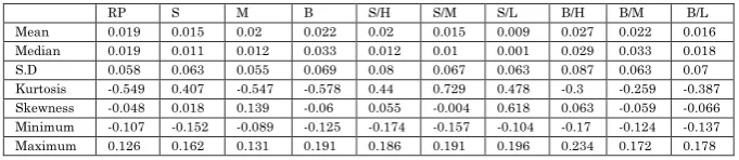
As shown in Table 2, return for overall portfolio (RP) is 0.019 whereas small size portfolios (S) have low returns, big size portfolio (B) has large returns, high price earning ratio (S/H and B/H)
Table 2: Descriptive Statistics (For 2002-2006)
RP S M B S/H S/M S/L B/H B/M B/L Mean 0.019 0.015 0.02 0.022 0.02 0.015 0.009 0.027 0.022 0.016 Median 0.019 0.011 0.012 0.033 0.012 0.01 0.001 0.029 0.033 0.018 S.D 0.058 0.063 0.055 0.069 0.08 0.067 0.063 0.087 0.063 0.07 Kurtosis -0.549 0.407 -0.547 -0.578 0.44 0.729 0.478 -0.3 -0.259 -0.387 Skewness -0.048 0.018 0.139 -0.06 0.055 -0.004 0.618 0.063 -0.059 -0.066 Minimum -0.107 -0.152 -0.089 -0.125 -0.174 -0.157 -0.104 -0.17 -0.124 -0.137 Maximum 0.126 0.162 0.131 0.191 0.186 0.191 0.196 0.234 0.172 0.178
negatively skewed. Kurtosis for all portfolios is platykurtic as the value of kurtosis is less than standard level of 3.
Table 3: Descriptive Statistics (For 2007-2011)
RP RP RP RP RP RP RP RP RP RP … S M B S/H S/M S/L B/H B/M B/L Mean -0.01 -0.01 -0.01 -0.01 -0.01 -0.004 -0.011 0 0 -0.007 Median -0.01 -0.01 -0.01 -0 -0.02 -0.012 -0.006 0.001 0.006 -0.008 S.D 0.051 0.06 0.05 0.07 0.085 0.063 0.064 0.106 0.085 0.056 Kurtosis 0.24 2.336 -0.05 0.725 2.296 2.255 2.402 3.038 1.564 -0.157 Skewness -0.41 -0.83 -0.18 -0.7 -0.38 -0.409 -0.583 -0.37 -0.094 -0.332 Minimum -0.14 -0.21 -0.13 -0.22 -0.29 -0.209 -0.239 -0.35 -0.226 -0.14 Maximum 0.1 0.132 0.1 0.121 0.213 0.153 0.16 0.349 0.252 0.11
As shown in Table 3, returns for all the portfolios are negative as -0.01 for the overall portfolio (RP) small sized portfolio(S) medium sized (M) big sized (B) and high price earning portfolios respectively. The returns of portfolios S/M, S/L and B/L are -.004, -.011 and -.007 respectively whereas for high price earning (B/H) and medium price earning (B/M) are 0. All the portfolios are negatively skewed having the values of 0.14, 0.21, 0.13, 0.22, 0.29, 0.209, 0.239, 0.35, 0.226, and 0.14 for the RP, S, M, B, S/H, S/M, S/L, B/H, B/M and B/L respectively. Kurtosis for all the portfolios is platykurtic as the value is not at the standard level of 3.The maximum gain is 0.349 incurred by the portfolio high price earning portfolio (B/H) and the minimum loss is incurred by the medium sized portfolio (M).
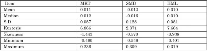
Table 4: Descriptive Statistics of Fama and French Three Factors
Item MKT SMB HML
Mean 0.011 -0.012 0.010
Median 0.012 -0.016 0.010
S.D 0.087 0.128 0.081
Kurtosis 6.866 2.371 7.664
Skewness -1.443 -0.570 -0.938
Minimum -0.460 -0.546 -0.401
Maximum 0.236 0.309 0.319
compared to size and value premium. It may be the effect of exceptional performance of Pakistani equity market during the period. Value stocks perform better than the growth stocks as it represented by positive value premium (HML). Negative size premium (SMB) indicates that big stocks average is higher than that of the small stocks.
Table 5 Correlation Matrix (For the Period of 2002 to 2011)
RP S M B S/H S/M S/L B/H B/M B/L
Rm-Rf 0.717 0.515 0.608 0.796 0.493 0.431 0.466 0.713 0.703 0.628 SMB -0.007 0.378 0.101 -0.467 0.230 0.405 0.375 -0.280 -0.563 -0.434 HML 0.333 0.272 0.215 0.421 0.320 0.268 0.076 0.751 0.247 -0.040
For Period of 2002 to 2006
RP S M B S/H S/M S/L B/H B/M B/L
Rm-Rf 0.738 0.559 0.650 0.850 0.457 0.516 0.623 0.786 0.833 0.811 SMB -0.010 0.341 0.042 -0.384 0.315 0.367 0.199 -0.299 -0.440 -0.389 HML 0.326 0.306 0.301 0.311 0.382 0.312 0.094 0.538 0.286 -0.024
For the Period of 2007 to 2011
RP S M B S/H S/M S/L B/H B/M B/L
Rm-Rf 0.680 0.443 0.530 0.738 0.483 0.324 0.304 0.652 0.610 0.426 SMB 0.002 0.439 0.163 -0.544 0.196 0.465 0.514 -0.271 -0.630 -0.518 HML 0.372 0.271 0.179 0.506 0.302 0.262 0.062 0.868 0.230 -0.073
portfolio (RP) to low price earning portfolios (B/L) for the sub period of 2002-2006. Size premium (SMB) is negatively correlated to the average returns of overall portfolio (RP), big sized portfolio B, high price earning portfolio (B/H), medium sized portfolio (B/M) and low price earning portfolio (B/L).Value premium is significantly positively correlated with the average returns of all the portfolios like overall portfolio (RP), small sized portfolio (S), medium sized (M), high price earning portfolios(S/H, B/H). For the period of 2007 to 2011, market premium (Rm-Rf) is positively correlated with the returns of all the portfolios from overall portfolio (RP) to low price earning portfolio (B/L).Size premium is positively correlated with the returns of the portfolios except big sized (B), high price earning (B/H), medium price earning (B/M) and low price earning (B/L). Value premium (HML) is also positively correlated with the returns of all portfolios. It is negatively correlated only with the portfolio low price earning portfolio (B/L).
Table 6 Regression Analysis with Rm-Rf (For the Period 2002 to 2011)
RP S M B S/H S/M S/L B/H B/M B/L Coefficients 0.000 -0.001 0.000 0.001 -0.001 0.002 -0.005 0.004 0.004 -0.001 MP* 0.463 0.369 0.393 0.648 0.477 0.326 0.344 0.804 0.609 0.462 T-Value 11.162 6.524 8.310 14.293 6.157 5.189 5.728 11.051 10.737 8.771 P-Value 0.000 0.000 0.000 0.000 0.000 0.000 0.000 0.000 0.000 0.000 Adj. R2 0.510 0.259 0.364 0.631 0.237 0.179 0.211 0.504 0.490 0.390
*MP is Market Premium
As shown in Table 6, the value of adjusted R2 is 0.510, 0.259,
premium has significant linear relationship with the stock returns and it is unfailing with CAPM.
Table 7 Regression on Rm-Rf and SMB (For the Period of 2002 to 2011)
Market Premium Size Premium
Coef. MP* T-Value P-Value SP** T-Value P-Value Adj. R2
RP 0.001 0.510 -12.30 0.000 0.103 -3.671 0.000 0.556
S 0.001 0.499 -11.12 0.000 0.287 -9.451 0.000 0.576
M 0.001 0.456 -9.89 0.000 0.139 -4.457 0.000 0.452
B 0.000 0.587 -13.28 0.000 -0.135 -4.507 0.000 0.683
S/H 0.001 0.602 -8.31 0.000 0.276 -5.631 0.000 0.394
S/M 0.004 0.464 -8.98 0.000 0.304 -8.690 0.000 0.497
S/L -0.003 0.474 -9.49 0.000 0.286 -8.456 0.000 0.506
B/H 0.004 0.781 -10.21 0.000 -0.050 -0.975 0.000 0.504
B/M 0.002 0.507 -9.86 0.000 -0.224 -6.443 0.000 0.620
B/L -0.001 0.402 -7.64 0.000 -0.132 -3.708 0.000 0.449
*MP stands for Market Premium; **SP stands for Size Premium
As shown in Table 7, due to incorporation of one additional factor i.e. size premium leads to an increase in adjusted R2 in
all portfolios except high price earning portfolio (B/H). It means that size effect is present in all portfolios. Similarly size premium (SMB) is found significant for small portfolios returns and it is found insignificant for portfolio high price earning portfolio (B/H). It means that size premium (SMB)is not significantly influence the returns of big size and high price earning portfolios. Market premium is also found significant for all the portfolios and it is consistent with the conventional Capital Asset Pricing Model. So market factor can significantly explain the equity returns and size premium can better explain the returns for small portfolios.
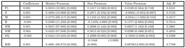
Table 8 Regression on Rm-Rf, SMB and HML (For the Period 2002 to 2011)
Coefficients Market Premium Size Premium Value Premium Adj. R2
P1 0.001 0.5033 (10.991) [0.000] 0.1017 (3.580) [0.001] 0.0169 (0.364) [0.716] 0.5531 S 0.001 0.4994 (10.069) [0.000] 0.2871 (9.332) [0.000] -0.0002 (-0.004) [0.997] 0.5725 M 0.001 0.4775 (09.417) [0.000] 0.1432 (4.552) [0.000] -0.0524 (-1.020) [0.310] 0.4517 B -0.001 0.5300 (11.250) [0.000] -0.1455(-4.980) [0.000] 0.1377 (2.885) [0.005] 0.7014 S/H 0.001 0.5637 (07.085) [0.000] 0.2686 (5.442) [0.000] 0.0937 (1.162) [0.248] 0.3961 S/M 0.004 0.4525 (07.936) [0.000] 0.3015 (8.525) [0.000] 0.0286 (0.496) [0.621] 0.4935 S/L -0.002 0.5424 (10.225) [0.000] 0.2989 (9.085) [0.000] -0.1659 (3.088) [0.003] 0.5396
B/H 0.001 0.4981 (08.873) [0.000]
-0.1048 (-3.009)
B/M 0.002 0.5024 (08.847) [0.000] 0.225(-6.387) [0.000] 0.0109 (0.189) [0.850] 0.6171
B/L 0.001 0.5034 (09.413) [0.000]
-0.1124 (-3.387)
[0.000] -0.2472 (4.562) [0.000] 0.5288 ( ) shows T-Value and [ ] shows P-Value
As shown in Table 8, value premium is positive and significant for portfolios (B/L) but negatively significant for B/H and S/L. It is insignificant for the overall portfolio (RP) and individual portfolios S/H, S/M and B/L. Incorporation of value premium leads to an increase in the value of adjusted R2 for the portfolios
S/L, B/H and B/L. It means that value premium effect is present in these portfolios. In this period it mostly explains the low price earning stocks.
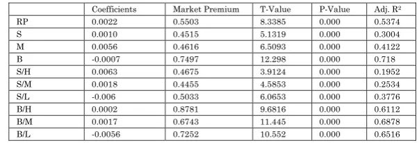
Table 9 Regression on Rm-Rf (For the Period of 2002 to 2006)
Coefficients Market Premium T-Value P-Value Adj. R2
RP 0.0022 0.5503 8.3385 0.000 0.5374 S 0.0010 0.4515 5.1319 0.000 0.3004 M 0.0056 0.4616 6.5093 0.000 0.4122 B -0.0007 0.7497 12.298 0.000 0.718 S/H 0.0063 0.4675 3.9124 0.000 0.1952 S/M 0.0018 0.4455 4.5853 0.000 0.2534 S/L -0.006 0.5033 6.0653 0.000 0.3776 B/H 0.0002 0.8781 9.6816 0.000 0.6112 B/M 0.0017 0.6743 11.445 0.000 0.6878 B/L -0.0056 0.7252 10.552 0.000 0.6516
As shown in Table 9, market premium shows the significant results for all the portfolios for the period of 2002 to 2006. Adjusted R2 for the overall portfolio is 0.5374.
Table 10 Regression on Rm-Rf and SMB (For the Period of 2002 to 2006)
Coefficients Market Premium Size Premium Adj. R2
Rp 0.0021
0.6528 0.1975
0.6309 (-10.141)[0.000] (-3.9628) [0.002]
S 0.0007
0.6704 (10.356) [0.000]
0.4216
0.6825 (8.4132) [0.000]
M 0.0055
0.5649 (8.0360) [0.000]
0.1991
0.5156 (-3.658) [0.006]
B -0.0006
0.7319 (10.940) [0.000]
-0.0343
0.7153 (-0.6619) [0.511]
SH 0.006
0.7122 (6.8466) [0.000]
0.4714
0.4885 (5.8537) [0.000]
SM 0.0015
0.6832 (9.3717) [0.000]
0.458
0.6475 (8.1144) [0.000]
(9.5162) [0.000] (6.084) [0.000]
BH 0.0002
0.8869 (8.8803) [0.000]
0.017
0.6047 (-0.2193) [0.827]
BM 0.0018
0.6335 (9.9768) [0.000]
-0.0787
0.696 (-1.6013) [0.115]
BL -0.0055
0.698 (9.2848) [0.000]
0.0524
0.6505 (-0.899) [0.372]
( ) shows T-value and [ ] shows P-value
As shown in Table 10, the addition of size premium is positive for all portfolios except B, BH, BM and BL. It means that SMB not significantly explain the returns of big size portfolios. Size premium leads to an increase in the value of adjusted R2 for all
portfolios except B and BH.
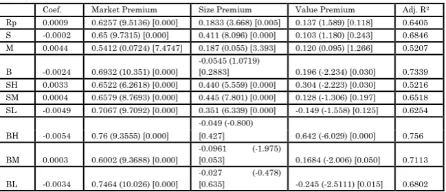
Table 11 Regression on Rm-Rf, SMB and HML (For the Period 2002 to 2006)
Coef. Market Premium Size Premium Value Premium Adj. R2
Rp 0.0009 0.6257 (9.5136) [0.000] 0.1833 (3.668) [0.005] 0.137 (1.589) [0.118] 0.6405 S -0.0002 0.65 (9.7315) [0.000] 0.411 (8.096) [0.000] 0.103 (1.180) [0.243] 0.6846 M 0.0044 0.5412 (0.0724) [7.4747] 0.187 (0.055) [3.393] 0.120 (0.095) [1.266] 0.5207
B -0.0024 0.6932 (10.351) [0.000]
-0.0545 (1.0719)
[0.2883] 0.196 (-2.234) [0.030] 0.7339 SH 0.0033 0.6522 (6.2618) [0.000] 0.440 (5.559) [0.000] 0.304 (-2.223) [0.030] 0.5216 SM 0.0004 0.6579 (8.7693) [0.000] 0.445 (7.801) [0.000] 0.128 (-1.306) [0.197] 0.6518 SL -0.0049 0.7067 (9.7092) [0.000] 0.351 (6.339) [0.000] -0.149 (-1.558) [0.125] 0.6254
BH -0.0054 0.76 (9.3555) [0.000]
-0.049 (-0.800)
0.642 (-6.029) [0.000] 0.756 [0.427]
BM 0.0003 0.6002 (9.3688) [0.000]
-0.0961 (-1.975)
[0.053] 0.1684 (-2.006) [0.050] 0.7113
BL -0.0034 0.7464 (10.026) [0.000]
-0.027 (-0.478)
[0.635] -0.245 (-2.5111) [0.015] 0.6802
As shown in Table 11, in this sub period of 2002 to 2006 market premium is significant for all the portfolios except portfolio (complete name) (M). In this period size premium is insignificant for the portfolios M, B, B/H and B/L. It means that in the period of 2002-2006 size premium factor is unable to significantly influence the returns of big stocks. Value premium is positive and significant for S/H but negatively significant for the B/H and B/L. It means that in the period of 2002-2006 HML can better explain the returns of these stocks. In addition in this period there is an increase in the value of adjusted R2 for
present in the sub period 2002-2006. In this period it explains the high price earning stocks.
Table 12 Regression on Rm-Rf(For the Period of 2007 to 2011)
Coefficients Market Premium T-Value P-Value Adj. R2
RP -0.005 0.380 7.057 0.000 0.453
S -0.006 0.289 3.768 0.000 0.183
M -0.009 0.305 4.757 0.000 0.268
B -0.002 0.566 8.325 0.000 0.537
S/H -0.008 0.451 4.200 0.000 0.220
S/M -0.003 0.222 2.606 0.012 0.089
S/L -0.009 0.213 2.433 0.018 0.077
B/H 0.006 0.757 6.541 0.000 0.415
B/M 0.004 0.563 5.856 0.000 0.361
B/L -0.005 0.258 3.585 0.001 0.167
As shown in Table 12, market premium is significant for all portfolios in the sub period of 2007-2011. The minimum value of the adjusted R2 is for the portfolio S/L.
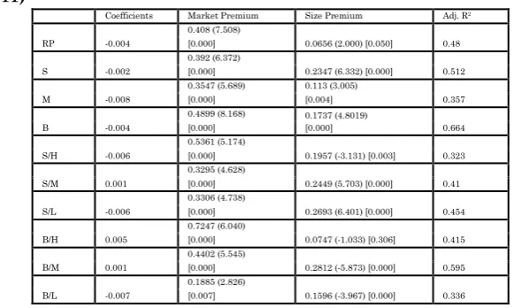
Table 13 Regression on Rm-Rf and SMB (For the Period of 2007 to 2011)
Coefficients Market Premium Size Premium Adj. R2
RP -0.004
0.408 (7.508)
0.0656 (2.000) [0.050] 0.48 [0.000]
S -0.002
0.392 (6.372)
0.2347 (6.332) [0.000] 0.512 [0.000]
M -0.008
0.3547 (5.689) 0.113 (3.005)
0.357 [0.000] [0.004]
B -0.004
0.4899 (8.168) 0.1737 (4.8019)
[0.000] 0.664 [0.000]
S/H -0.006
0.5361 (5.174)
0.1957 (-3.131) [0.003] 0.323 [0.000]
S/M 0.001
0.3295 (4.628)
0.2449 (5.703) [0.000] 0.41 [0.000]
S/L -0.006
0.3306 (4.738)
0.2693 (6.401) [0.000] 0.454 [0.000]
B/H 0.005
0.7247 (6.040)
0.0747 (-1.033) [0.306] 0.415 [0.000]
B/M 0.001
0.4402 (5.545)
0.2812 (-5.873) [0.000] 0.595 [0.000]
B/L -0.007
0.1885 (2.826)
0.1596 (-3.967) [0.000] 0.336 [0.007]
As shown in Table 13, size premium is significant for all the portfolios exceptBH. There is also an increase in the value of adjusted R2 except in portfolio BH. It means that size premium
Table 14 Regression on Rm-Rf, SMB and HML (For the Period 2007 to 2011)
Coefficients Market Premium Size Premium Value Premium Adj. R2
RP -0.004
0.4028 (6.321) [0.000]
0.065 (1.953) [0.056]
0.0091 (0.165) [0.870] 0.471
S -0.002
0.3948 (5.479) [0.000]
0.235 (6.248) [0.000]
-0.0053 (-0.085) [0.932] 0.503
M -0.007
0.4027 (5.592) [0.000]
0.1184 (3.150) [0.003]
-0.0817 (-1.309) [0.196] 0.365
B -0.006
0.3964 (6.014) [0.000]
-0.1843 (-5.3552) [0.000]
0.1592 (2.786) [0.007] 0.7
S/H -0.006
0.5178 (4.265) [0.000]
0.1936 (3.054) [0.003]
0.0312 (0.297) [0.768] 0.312
S/M 0.001
0.3075 (3.693) [0.000]
0.2424 (5.575) [0.000]
0.0373 (0.516) [0.608] 0.402
S/L -0.004
0.4053 (5.102) [0.000]
0.2778 (6.698) [0.000]
-0.127 (-1.844) [0.071] 0.476
B/H -0.004
0.2672 (3.640) [0.000]
-0.1264 (3.2982) [0.002]
0.7785 (12.229) [0.000] 0.838
B/M 0.001
0.4592 (4.941) [0.000]
-0.279 (-5.750) [0.002]
-0.0324 (-0.402) [0.689] 0.589
B/L 0.005
0.2954 (4.046) [0.000]
-0.1475 (-3.869) [0.000]
-0.1819 (-2.874) [0.006] 0.411
As shown in Table14, market premium is significant for all the portfolios which shows the explanatory power of this factor during the period 2007-2011. Size premium is significant for all the portfolios during this period. It means that SMB significantly influence the returns of stocks during the period of 2007-2011. HML is positively significant for the B/L but negatively significant for the significant B/H. It means that during the period HML can better explain the returns of these portfolios. There is only increase in the value of adjusted R2 of
portfolios S/L, B/H and B/L. So it is concluded that in this period it again explaining the low price earning stocks.
Conclusion:
period of 2002 to 2011 and sub periods of 2002 to 2006 and 2007 to 2011. These findings are consistent with the conventional CAPM and it is valid in Pakistani equity market under the assumption studied period. The results of size premium exhibit that in the period of 2002 to 2011 it is found insignificant for the portfolio B/H whereas for the period of 2002 to 2006 it is significant for all the portfolios excluding B and B/H. In the sub period 2007 to 2011 it is again insignificant for the portfolio B/H. It means that size premium does not explain the returns of big stocks. The findings of the study are in line with the two earlier studies in Pakistani equity market conducted by Hassan and Javed (2011) who concluded that size premium is insignificant for the big portfolios. By comparing the regression results of value premium in all the periods it is clear that the effect of value premium is present in Pakistani equity market. In the period of 2002 to 2011 and for both sub periods HML explains the low price earning stocks but in sub period of 2002-2006 it explains the high price earning stocks. As the results of the two periods are same so it is concluded that HML explains the low price earning stocks. The results are in consistent with the Hassan and Javed (2011) that the effect of value premium is present in Pakistani equity market. Price earning is a negative proxy of book to market in this study.
REFERENCES:
1. Aleati, A., Gottardo. P, & Murgia, M. (2000). The Pricing of Italian Equity Returns. Economic Notes, Vol.29, 153-177.
2. Basu, S. (1977). Investment performance of common stocks in relation to their price‐earnings ratios: A test of
3. Basu, S. (1983). The relationship between earnings' yield, market value and return for NYSE common stocks: Further evidence. Journal of financial economics, 12(1), 129-156.
4. Banz, R. W. (1981). The relationship between return and market value of common stocks. Journal of financial economics, 9(1), 3-18.
5. Barber, B. M., & Lyon, J. D. (1997). Firm Size, Book‐to‐Market Ratio, and Security Returns: A Holdout
Sample of Financial Firms. The Journal of Finance, 52(2), 875-883.
6. Black, F. (1972). Capital market equilibrium with restricted borrowing. The Journal of Business, 45(3), 444-455.
7. Cox, J. C., Ingersoll Jr, J. E., & Ross, S. A. (1985). An Intertemporal general equilibrium model of asset prices. Econometrica: Journal of the Econometric Society, 363-384.
8. Daniel, K., & Titman, S. (March 1997). Evidence on the Characteristics of Cross Sectional Variation in Stock Returns. The Journal of Finance, Vol. LII, No. 5.
9. Drew, M. E., Naughton, T., & Veeraraghavan, M. (2003). Firm Size, Book-To-Market Equity and Security Returns: Evidence from the Shanghai Stock Exchange. Australian Journal of Management, Vol. 28, No.2, 1-22. 10.Faff, R. (2001). An examination of the Fama and French
three-factor model using commercially available factors. Australian Journal of Management, 26(1), 1-17.
11.Fama, E. F., & MacBeth, J. D. (1973). Risk, return, and equilibrium: Empirical tests. The Journal of Political Economy, 607-636.
13.Fama, E. F., & French, K. R. (1993). Common Risk Factors in the Returns on the Stocks and Bonds. The Journal of Finance, 3, 3-56.
14.Fama, E. F., & French, K. R. (1995). Size and book‐to‐market factors in earnings and returns. The
Journal of Finance, 50(1), 131-155.
15.Fama, E. F., & French, K. R. (1996). Multifactor explanations of asset pricing anomalies. The journal of finance, 51(1), 55-84.
16.Fama, E. F., & French, K. R. (1998). Value versus growth: The international evidence. The Journal of Finance, 53(6), 1975-1999.
17.Gaunt, C. (2004). Size and Book to Market Effects and the Fama French Three Factor Asset Pricing Model: Evidence from the Australian Stockmarket. Accounting and Finance, Vol.44,27-44.
18.Hassan, A., & Javed, M. T. (2011). Size and Value Premium in Pakistani Equity Market. African Journal of Business Management, Vol.5,No.16, 47-56.
19.Louis K. C. Chan, Y. H. (1991). Fundamentals and Stock Returns in Japan. The Journal of Finance, Vol. XLVI, No. 5, 1-27.
20.Lewellen, J. (1999). The Time-Series Relations among Expected Return, Risk, and Book-To-Market. Journal of Financial Economics, Vol.53, 5-43.
21.Jacobs, B. I., & Levy, K. N. (1988). Disentangling equity return regularities: New insights and investment opportunities. Financial Analysts Journal, 18-43.
22.Jegadeesh, N., & Titman, S. (1993). Returns to buying winners and selling losers: Implications for stock market efficiency. The Journal of Finance, 48(1), 65-91.
24.Lintner, J. (1965). Security prices, risk, and maximal gains from diversification. The Journal of Finance, 20(4), 587-615.
25.Markowitz, H. (1952). Portfolio selection. The journal of finance, 7(1), 77-91.
26.Merton, R. C. (1973). An intertemporal capital asset pricing model. Econometrica: Journal of the Econometric Society, 867-887.
27.Mossin, J. (1966). Equilibrium in a capital asset market. Econometrica: Journal of the Econometric Society, 768-783.
28.Ross, S. A. (1976). The arbitrage theory of capital asset pricing. Journal of economic theory, 13(3), 341-360. 29.Rubinstein, M. (1976). The valuation of uncertain
income streams and the pricing of options. The Bell Journal of Economics, 407-425.
30.Rosenberg, B., Reid, K., & Lanstein, R. (1985). Persuasive evidence of market inefficiency. The Journal of Portfolio Management, 11(3), 9-16.
31.Ong, T. S., Yichen, Y. N., & Teh, B. H. (2010). Can High Price Earnings Ratio Act as an Indicator of the Coming Bear Market in the Malaysia. International Journal of Business and Social Science, Vol.1,No.1, 1-20.
32.Sharpe W, F. (1964). Capital asset prices: A theory of market equilibrium under conditions of risk. Journal of finance, 19(3), 425-442.
33.Stattman, D. (1980). Book values and stock returns. The Chicago MBA: A journal of selected papers, 4(1), 25-45. 34.Zeytinoglu, E., Akarim, Y. D., & Çelik, S. (2012). The