Numerical Method of Simulation of Material Influences in Mr Tomography

(1)

NUMERICAL METHOD OF SIMULATION OF MATERIAL INFLUENCES IN MR TOMOGRAPHY M. Steinbauer and R. Kubasek

Faculty of Electrical Engineering and Communications Brno University of Technology

Czech Republic

K. Bartusek

Institute of Scientiﬁc Instruments

Academy of Sciences of the Czech Republic Czech Republic

Abstract—Generally all Magnetic Resonance Imaging (MRI) tech-niques are affected by magnetic and electric properties of measured materials, resulting in errors in MR image. Using numerical simula-tion we can solve the effect of changes in homogeneity of static and RF magnetic fields caused by specimen made from conductive and/or magnetic material in MR tomograph. This paper deals with numerical simulation of material susceptibility influence to magnetic field.

1. INTRODUCTION

In MR tomography, strong magnetic field is used (above 1 T). Because MR is very sensitive to inhomogeneity of this field, even such weak induced magnetic field as from para- or diamagnetic material is significant. Second mechanism, which affects field homogeneity, is magnetic field off eddy current induced by RF impulse in conductive material. Aim of this paper is in simulation of weakly magnetic material influence to static magnetic field.

(2)

double precision arithmetic and sufficiently fine mesh, because change of the magnetic field in vicinity of slightly magnetic materials is weak in comparison to basic static magnetic field. Second approach may use single precision arithmetic, because only reactional field (induced own field of magnetic material) is computed.

2. 2D ANALYTIC SOLUTION

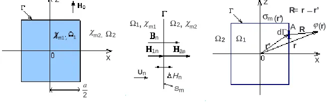
Let’s have specimen with susceptibility χm1 surrounded by reference medium with known susceptibility χm2 and placed into static primal magnetic ﬁeld with magnetic intensity vector H0 oriented in uz

direction — see Fig. 1 left. We have to determine magnetic intensity Hof incurred field, which is superposition of primal and reaction field Hr (effect of specimen magnetization).

m1, 1

m2,

m2, 1,

χ χ _Ω2

Ω1,χ_m1 Ω2,χm2,m2

2n n

1n

Hn

Un

z

x x

z

sm

2 2 Ω1

r’

d_Γ AR

R= r_r’

ϕ(r)

r

_

2 a

σm(r’)

Ω

Figure 1. 2D analytic model for rectangular specimen (left), replacement of specimen magnetization eﬀect by surface magnetic charge at the area boundaries (right) and boundary detail (middle).

Because there are not variable currents in whole area, magnetic ﬁeld is irrotational (rot H = 0) and we can use scalar magnetic potential

H=−gradϕm. (1) Magnetic potential of primal ﬁeld of intensityH0 is

ϕm0=−

(3)

∆H=H−H0

∆H(r) = 1 2π

Γ

σm(r) ur

R(r,r)dΓ. (3) Surface magnetic charge invokes scalar magnetic potential [5]

ϕmr(r) =− 1 2π

Γ

σm(r) lnR(r,r)dΓ. (4)

Total scalar magnetic potential at pointris superposition of static primal ﬁeld intensity (2) and contribution from charged bound (4)

ϕm(r) =−Hz− 1

2π

Γ

σm(r) lnR(r,r)dΓ. (5)

Using condition of magnetic ﬂux Bn = Bnun we obtain an integral formula for surface magnetic charge density normal component conjunction on bound Γ (see Fig. 1 middle)

Bn=µ0(1 +χm1)H1n=µ0(1 +χm2)H2n (6)

Analogically to the Gauss theorem causes magnetic charge of densityσmat point A magnetic ﬁeld of intensity

∆Hn =±

σm(A)

2 . (7)

Using (5) and (1) we have the normal components of magnetic ﬁeld intensity at point A (Fig. 1 middle)

H1n=H0uzun+

1 2πgrad

Γ, r∈Ω1

σm

rlnR(r,r)dΓun, (8)

H2n=H0uzun+

1 2πgrad

Γ, r∈Ω1

σm

rlnR(r,r)dΓun. (9)

Whenever A∈Γ and thusr ∈Γ, has integral in formulas (8) a (9) singularity at point A (wherer =r). We can remove this singularity omitting pointr=r from integration and taking ﬁeld contribution of this point using (7) instead. So we can write

H1n =H0uz·un+

1 2π

Γ

r=r

σm

r 1

R(r,r)dΓuR·un−

σm(A)

(4)

H2n =H0uz·un+ 1 2π

Γ

r=r

σm

r 1

R(r,r)dΓuR·un+

σm(A)

2 , (11)

where was used

grad lnR(r,r) = 1

R(r,r)uR. (12) Substituting from (10) and (11) into (6) we have after some rearrangement

χ∆ 2π

Γ

r∈Γ,r=r

σm(r)

R(r,r)dΓuR·un+

σm(r)

2 =−χ∆H0uz·un, (13)

where diﬀerential susceptibility was introduced

χ∆=

χm1−χm2

χm1+χm2+ 2

. (14)

Formula (13) is not analytically solvable, thus we solve it numerically by mean of boundary element method. After solution of (13) using collocation method described in [5] we have obtained results, shown in next ﬁgure. Shape of magnetic ﬂux density is in the Fig. 2. In this simulation the aluminium specimen (Ω1) was considered with χm1 = 22 · 10−6, length of specimen z = 20 mm, thickness

a= (3, 5 and 7) mm. Specimen was immersed into the water with

χm2=−9·10−6−(Ω2).

-0.2 -0.1 5 -0.1 -0.0 5 0 0.05 0.1 0.15 0. 2 -4

-2 0 2 4 6 8 10 12 14x 10

-5

x (m)

a= 7m m a=5mm a=3mm

b = 20mm

m1= 22e -6

χm2= -9 6

B(T)

χ

(5)

3. 3D NUMERICAL SOLUTION

Three dimensional numerical modeling was provided using FEM and Ansys software. The scalar magnetic potential was computed by solving of Laplace’s equation

∆ϕm= divµ(−gradϕm) = 0. (15)

One of used model is in Fig. 3. Here weakly paramagnetic specimen is surrounded by diamagnetic reference substance. The model was meshed with Solid96 element type. Boundary conditions were set up to achieve induction B0 = 4,700 T in z-axes direction:

ϕm=const.on the surfaces Γ1, Γ2, ∂ϕ_∂_nm = 0 on the shell surface Γ3.

m2

χ m1

m2 ,

1

3

4

2

χ

Figure 3. FEM model (left) and compute result (right) for magnetic ﬂux density.

FEM modeling and solution is described in [8]. One of obtained results — the module of magnetic inductionBalong the “path” marked in Fig. 3 — is shown in the ﬁgure in the right.

4. CONCLUSIONS

Both method of numerical modeling of magnetic ﬁeld deformation in MRI, caused by weakly magnetic specimen, which were described here, was compared with experimental results [3, 8]. Proximity of measured and numerically modeled data was good — see [5]. To enable comparison, simulation was adjusted to the same conditions as experiment: size of sample, susceptibilities and magnetic ﬁeld of B = 4.7 T.

(6)

tomography. The method uses Gradient Echo (GE) method and benefits from magnetic induction field shape in specimen vicinity, which is immersed in reference medium with measurable MR signal. After an optimization this method can be used for investigation of the materials used in MR tomography as well as of biological tissues affecting quality of MR images.

ACKNOWLEDGMENT

This work is supported by the grants GAAV B208130603 and GAAV B208130604.

REFERENCES

1. Ernst, R. R., G. Bodenhausen, and A. Wokaun,Principles of NMR in One and Two Dimensions, Oxford Science Publishing, 1987. 2. Sep´ulveda, N. G., I. M. Thomas, and J. P. Wikswo, Jr., “Magnetic

susceptibility tomography for three-dimensional imaging of diamagnetic and paramagnetic objects,” IEEE Transaction on Magnetics, Vol. 30, No. 6, 5062–5069, 1994.

3. Kubasek, R., M. Steinbauer, and K. Bartusek, “Material inﬂuences in MR tomography, measurement and simulation,” Journal of Electrical Engineering, Vol. 8, 58–61, Zilina, 2006. 4. Wang, Z. J., S. Li, and J. C. Hasselgrove, “Magnetic resonance

imaging measurement of volume magnetic susceptibility using a boundary condition,” Journal of Magnetic Resonance, Vol. 142, 477–481, 1999.

5. Hwang, S. N. and F. W. Wehrli, “Experimental evaluation of surface charge method for computing the induced magnetic ﬁeld in trabecular bone,” Journal of Magnetic Resonance, Vol. 139, 35–45, 1999.

6. Eastham, J. F., R. J. Hill-Cottingham, I. R. Young, and J. V. Hajnal, “A method of inverse calculation for regions of small susceptibility variations,”IEEE Transaction on Magnetics, Vol. 33, No. 2, 1212–1215, 1997.

7. Eastham, J. F., R. J. Hill-Cottingham, I. R. Young, J. V. Hajnal, P. J. Leonard, and W. Lin, “Use of ﬁnite element analysis to calculate ﬁeld changes in low susceptibility materials,”Proceedings

of Compumag 95 International Conference, 546–547, Berlin,

Germany, 1995.