Western University Western University
Scholarship@Western
Scholarship@Western
Electronic Thesis and Dissertation Repository
4-24-2014 12:00 AM
On The Parallelization Of Integer Polynomial Multiplication
On The Parallelization Of Integer Polynomial Multiplication
Farnam Mansouri
The University of Western Ontario
Supervisor
Dr. Marc Moreno Maza
The University of Western Ontario Graduate Program in Computer Science
A thesis submitted in partial fulfillment of the requirements for the degree in Master of Science © Farnam Mansouri 2014
Follow this and additional works at: https://ir.lib.uwo.ca/etd
Part of the Theory and Algorithms Commons
Recommended Citation Recommended Citation
Mansouri, Farnam, "On The Parallelization Of Integer Polynomial Multiplication" (2014). Electronic Thesis and Dissertation Repository. 2039.
https://ir.lib.uwo.ca/etd/2039
This Dissertation/Thesis is brought to you for free and open access by Scholarship@Western. It has been accepted for inclusion in Electronic Thesis and Dissertation Repository by an authorized administrator of
On The Parallelization Of Integer Polynomial
Multiplication
(Thesis format: Monograph)
by
Farnam Mansouri
Graduate Program in Computer Science
A thesis submitted in partial fulfillment
of the requirements for the degree of
Master of Science
The School of Graduate and Postdoctoral Studies
The University of Western Ontario
London, Ontario, Canada
Abstract
With the advent of hardware accelerator technologies, multi-core processors and
GPUs, much effort for taking advantage of those architectures by designing parallel
al-gorithms has been made. To achieve this goal, one needs to consider both algebraic complexity and parallelism, plus making efficient use of memory traffic, cache, and
re-ducing overheads in the implementations.
Polynomial multiplication is at the core of many algorithms in symbolic computation
such as real root isolation which will be our main application for now.
In this thesis, we first investigate the multiplication of dense univariate polynomials
with integer coefficients targeting multi-core processors. Some of the proposed methods
are based on well-known serial classical algorithms, whereas a novel algorithm is designed
to make efficient use of the targeted hardware. Experimentation confirms our theoretical
analysis.
Second, we report on the first implementation of subproduct tree techniques on
many-core architectures. These techniques are basically another application of polynomial
multiplication, but over a prime field. This technique is used in multi-point evaluation
and interpolation of polynomials with coefficients over a prime field.
Keywords. Parallel algorithms, High Performance Computing, multi-core machines,
Acknowledgments
First and foremost I would like to offer my sincerest gratitude to my supervisor, Dr
Marc Moreno Maza, who has supported me throughout my thesis with his patience and
knowledge. I attribute the level of my Masters degree to his encouragement and effort, and without him, this thesis would not have been completed or written.
Secondly, I would like to thank Dr. Sardar Anisul Haque, Ning Xie, Dr. Yuzhen
Xie, and Dr. Changbo Chen for working along with me and helping me complete this
research work successfully. Many thanks to Dr. J¨urgen Gerhard of Maplesoft for his help
and useful guidance during my internship. In addition, thanks to Svyatoslav Covanov
for reading this thesis and his useful comments.
Thirdly, all my sincere thanks and appreciation go to all the members from our
Ontario Research Centre for Computer Algebra (ORCCA) lab in the Department of
Computer Science for their invaluable support and assistance, and all the members of my thesis examination committee.
Finally, I would like to thank all of my friends and family members for their consistent
encouragement and continued support.
I dedicate this thesis to my parents for their unconditional love and support
Contents
List of Algorithms vii
List of Tables ix
List of Figures x
1 Introduction 1
1.1 Integer polynomial multiplication on multi-core . . . 2
1.1.1 Example . . . 4
1.2 Polynomial evaluation and interpolation on many-core . . . 6
1.2.1 Example . . . 7
2 Background 9 2.1 Multi-core processors . . . 9
2.1.1 Fork-join parallelism model . . . 10
2.2 The ideal cache model . . . 13
2.3 General-purpose computing on graphics processing units . . . 15
2.3.1 CUDA . . . 15
2.4 Many-core machine model . . . 18
2.4.1 Complexity measures . . . 19
2.5 Fast Fourier transform over finite fields . . . 20
2.5.1 Sch¨onhage-Strassen FFT . . . 21
2.5.2 Cooley-Tukey and Stockham FFT . . . 22
3 Parallelizing classical algorithms for dense integer polynomial multi-plication 26 3.1 Preliminary results . . . 27
3.2 Kronecker substitution method . . . 30
3.2.1 Handling negative coefficients . . . 31
3.3 Classical divide & conquer . . . 33
3.4 Toom-Cook algorithm . . . 36
3.5 Parallelization . . . 43
3.5.1 Classical divide & conquer . . . 43
3.5.2 4-way Toom-Cook . . . 44
3.5.3 8-way Toom-Cook . . . 47
3.6 Experimentation . . . 50
3.7 Conclusion . . . 54
4 Parallel polynomial multiplication via two convolutions on multi-core processors 56 4.1 Introduction . . . 56
4.2 Multiplying integer polynomials via two convolutions . . . 58
4.2.1 Recoveringc(y) fromC+(x, y)and C−(x, y) . . . 62
4.2.2 The algorithm in pseudo-code . . . 64
4.2.3 Parallelization . . . 65
4.3 Complexity analysis . . . 66
4.3.1 Smooth integers in short intervals . . . 69
4.3.2 Proof of Theorem 1 . . . 70
4.4 Implementation . . . 70
4.5 Experimentation . . . 71
4.6 Conclusion . . . 74
5 Subproduct tree techniques on many-core GPUs 75 5.1 Introduction . . . 75
5.2 Background . . . 77
5.3 Subproduct tree construction . . . 80
5.4 Subinverse tree construction . . . 84
5.5 Polynomial evaluation . . . 89
5.6 Polynomial interpolation . . . 91
5.7 Experimentation . . . 94
5.8 Conclusion . . . 96
A Converting 106 A.1 Convert-in . . . 106
B Good N Table 109
List of Algorithms
1 Sch¨onhageStrassen . . . 21
2 Schoolbook(f, g, m, n) . . . 27
3 KroneckerSubstitution(f, g, m, n) . . . 31
4 Divide&Conquer(f, g, m, n, d) . . . 34
5 Recover(H, β, size) . . . 39
6 ToomCookK(f, g, m) . . . 39
7 Evaluate4(F) . . . 45
8 Interpolate4(c) . . . 46
9 SubproductTree(m0, . . . , mn−1) . . . 78
10 Inverse(f, `) . . . 80
11 TopDownTraverse(f, i, j, Mn, F) . . . 84
12 OneStepNewtonIteration(f, g, i) . . . 86
13 EfficientOneStep(Mi,j′ ,InvMi,j, i) . . . 87
14 InvPolyCompute(Mn,InvM,i, j) . . . 87
15 SubinverseTree(Mn, H) . . . 87
16 FastRemainder(a, b) . . . 92
17 LinearCombination(Mn, c0, . . . , cn−1) . . . 92
List of Tables
2.1 Table showing CUDA memory hierarchy [56] . . . 17
3.1 Intel node . . . 51
3.2 AMD node . . . 51
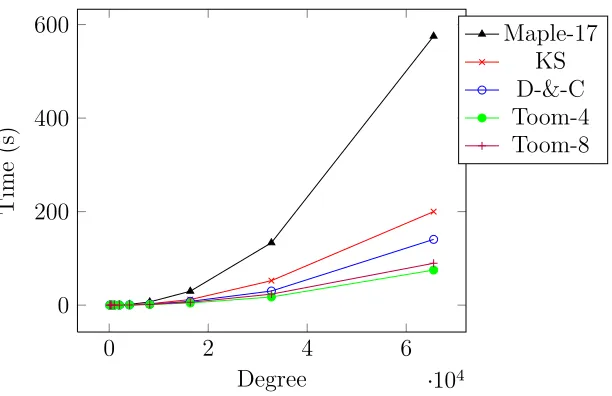
3.3 Execution times for the discussed algorithms. The size of the input poly-nomials (s) equals to the number of bits of their coefficients (N). The error for the largest input in Kronecker-substitution method is due to memory allocation limits. (Times are in seconds.) . . . 51
3.4 Execution times for the discussed algorithms compared with Maple-17 which also uses Kronecker-substitution algorithm. . . 51
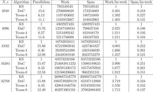
3.5 Cilkviewanalysis of the discussed algorithms for problems having differ-ent sizes (The size of the input polynomials (s) equals to the number of bits of their coefficientsN). The columnswork, and span are showing the number of instructions, and theparallelismis the ratio ofWork/Span. The work and span of each algorithm are compared with those of Kronecker-substitution method which has the best work. . . 53
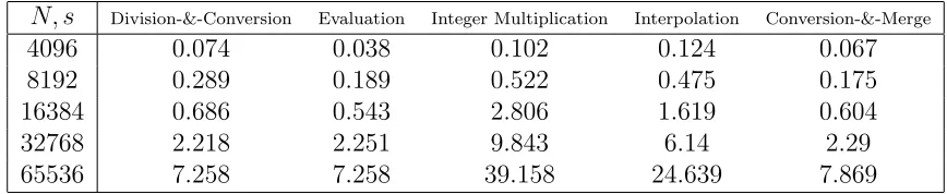
3.6 Profiled execution times for different sections of the algorithm in the 4-way Toom-Cook method. (Times are in seconds.) . . . 54
3.7 Profiled execution times for different sections of the algorithm in the 8-way Toom-Cook method. (Times are in seconds.) . . . 54
4.1 Polynomial multiplication timings withd=N. . . 71
4.2 Polynomial multiplication timings withd≪N. . . 72
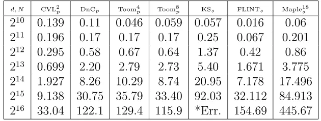
4.3 Profiling information for CVL2s and CVL2p. . . 72
4.4 Cilkviewanalysis of CVL2p and KSs. . . 72
5.1 Computation time for random polynomials with different degrees (2K)
and points. Teva and Tmul are running times for polynomial evaluation, an
polynomial multiplication (FFT-based) respectively. All of the times are
in seconds. . . 95
5.2 Effective memory bandwidth in (GB/S). k is log2 of the size of the input polynomial (n=2k). . . 95
5.3 Execution times of our FFT-based polynomial multiplication of polyno-mials with the size 2k comparing with FLINT library. . . 96
5.4 Execution times of our polynomial evaluation and interpolation where the size of polynomial is 2k compared with those of FLINT library. . . 97
B.1 Good N, k = log2K, M using two 62-bits primes. . . 109
B.2 Good N, k = log2K, M using two 62-bits primes. (Continue) . . . 110
List of Figures
1.1 Subproduct tree for evaluating a polynomials of degree 7 at 8 points. . . . 7
1.2 Top-down remaindering process associated with the subproduct tree for evaluating the example polynomial. The % symbol meansmod operation. Mi,j is the j-th polynomial at level iof the subproduct tree. . . 8
2.1 The ideal-cache model. . . 13
2.2 Scanning an array of n=N elements, withL=B words per cache line. . . 14
2.3 Illustration of the CUDA memory hierarchy [56] . . . 16
5.1 Subproduct tree associated with the point set U = {u0, . . . , un−1}. . . 78
5.2 Our GPU implementation versus FLINT for FFT-based polynomial mul-tiplication. . . 96
5.3 Interpolation lower degrees . . . 97
5.4 Interpolation higher degrees . . . 97
5.5 Evaluation lower degrees . . . 97
Chapter 1
Introduction
Polynomial multiplication and matrix multiplication are at the core of many algorithms
in symbolic computation. Expressing, in terms of multiplication time, the algebraic
complexity of an operation like univariate polynomial division or the computation of a
characteristic polynomial is a standard practice, see for instance the landmark book [29].
At the software level, the motto “reducing everything to multiplication”1is also common,
see for instance the computer algebra systems Magma2 [6], NTL3 or FLINT4.
With the advent of hardware accelerator technologies, multi-core processors and
Graphics Processing Units (GPUs), this reduction to multiplication is, of course, still
desirable, but becomes more complex since both algebraic complexity and parallelism need to be considered when selecting and implementing a multiplication algorithm. In
fact, other performance factors, such as cache usage or CPU pipeline optimization, should
be taken into account on modern computers, even on single-core processors. These
ob-servations guide the developers of projects like SPIRAL5 [57] or FFTW6 [20].
In this thesis, we investigate the parallelization of polynomial multiplication on both
multi-core processors and many-core GPUs. In the former case, we consider dense
poly-nomial multiplication with integer coefficients. The parallelization of this operation was
recognized as a major challenge for symbolic computation during the 2012 edition of the
East Coast Computer Algebra Day7. A first difficulty comes from the fact that, in a
computer memory, dense polynomials with arbitrary-precision coefficients cannot be rep-resented by a segment of contiguous memory locations. A second difficulty follows from
1Quoting a talk title by Allan Steel, from the Magma Project. 2Magma: http://magma.maths.usyd.edu.au/magma/
3NTL:http://www.shoup.net/ntl/ 4FLINT:http://www.flintlib.org/ 5http://www.spiral.net/
6http://www.fftw.org/ 7
the fact that the fastest serial algorithm for dense polynomial multiplication are based
on Fast Fourier Transforms (FFT) which, in general, is hard to parallelize on multi-core
processors.
In the case of GPUs, our study shifts to parallel dense polynomial multiplication
over finite fields and we investigate how this operation can be integrated into
high-level algorithm, namely those based on the so-called subproduct tree techniques. The
parallelization of these techniques is also recognized as a challenge that, before our work and to the best of our knowledge, has never been handled successfully. One reason is that
the polynomial products involved in the construction of a subproduct tree cover a wide
range of sizes, thus, making a naive parallelization hard, unless each of these products is
itself computed in a parallel fashion. This implies having efficient parallel algorithms for
multiplying small size polynomials as well as large ones. This latter constraint has been
realized on GPUs and is reported in a series of papers [53, 36].
We note that the parallelization of sparse(both univariate and multivariate)
polyno-mial multiplication on both multi-core processors and many-core GPUs has already been
studied by Gastineau & Laskard in [26, 27, 25], and by Monagan & Pearce in [51, 50].
Therefore, throughout this thesis, we focus on dense polynomials.
For multi-core processors, the case of modular coefficients was handled in [46, 47] by
techniques based on multi-dimensional FFTs. Considering now integer coefficients, one
can reduce to the univariate situation via Kronecker’s substitution, see for instance the implementation techniques proposed by Harvey in [39]. Therefore, we concentrate our
efforts on the univariate case.
1.1
Integer polynomial multiplication on multi-core
A first natural parallel solution for multiplying univariate integer polynomials is to
con-sider divide-and-conquer algorithms where arithmetic counts are saved thanks to the use of evaluation and interpolation techniques. Well-know instances of this solution are the
multiplication algorithms of Toom & Cook, among which Karatsuba’s method is a
spe-cial case. As we shall see with the experimental results of Section 3.6, this is a practical
solution. However, the parallelism is limited by the number of ways in the recursion.
Moreover, increasing the number of ways makes implementation quite complicated, see
the work by Bodrato and Zanoni for the case of integer multiplication [5, 69, 70]. As
in their work, our implementation includes the 4-way and 8-way cases. In addition, we
O(N logN) for the input size N).
Turning our attention to this latter class, we first considered combining Kronecker’s
substitution (so as to reduce multiplication in Z[x] to multiplication in Z) and the
algorithm of Sch¨onhage & Strassen [58]. The GMP-library8 provides indeed a highly
optimized implementation of this latter algorithm [30]. Despite of our efforts, we could
not obtain much parallelism from the Kronecker substitution part of this approach. It
became clear at this point that, in order to go beyond the performance (in terms of
arith-metic count and parallelism) of our parallel 8-way Toom-Cook code, our multiplication code had to rely on a parallel implementation of FFTs. These attempts to obtain an
efficient parallel algorithmic solution for dense polynomial multiplication over Z, from
serial algorithmic solutions, such as 8-way Toom-Cook, are reported in Chapter 3.1.
Based on the work of our colleagues from the SPIRAL and FFTW projects, and based
on our experience on the subject of FFTs [46, 47, 49], we know that an efficient way to
parallelize FFTs on multi-core architectures is the so-calledrow-columnalgorithms9which
implies to view 1-D FFTs as multi-dimensional FFTs and thus abandon the approach of Sch¨onhage & Strassen.
Reducing polynomial multiplication in Z[y] to multi-dimensional FFTs over a finite
field, say Z/pZ, implies transforming integers to polynomials over Z/pZ. As we shall
see in Section 4.5, this change of data representation can contribute substantially to the
overall running time. Therefore, we decided to invest implementation efforts in that
direction. We refer the reader to our publicly available code10.
In Chapter 4, we propose an FFT-based algorithm for multiplying dense polynomials
with integer coefficients in a parallel fashion, targeting multi-core processor architectures.
This algorithm reduces univariate polynomial over Z to 2-D FFT over a finite field
of the form Z/pZ. This addresses the performance issues raised above. In addition,
in our algorithm, the transformations between univariate polynomials over Z and
2-D arrays over Z/pZ require only machine word addition and shift operation. Thus,
our algorithm does not require to multiply integers at all. Our experimental results
show that, for sufficiently large input polynomials, on sufficiently many cores, this new
algorithm outperforms all other approaches mentioned above as well as the parallel dense
polynomial multiplication overZimplemented in FLINT. This new algorithm is presented in a paper [10] accepted at the International Symposium on Symbolic and Algebraic
Computation (ISSAC 2014)11. This is a joint work with Changbo Chen, Marc Moreno
8https://gmplib.org/
9http://en.wikipedia.org/wiki/Fast_Fourier_transform 10BPAS library: http://www.bpaslib.org/
11
Maza, Ning Xie and Yuzhen Xie. Our code is part of the Basic Polynomial Algebra
Subprograms (BPAS)12.
1.1.1
Example
We illustrate below the main ideas of this new algorithm for multiplying dense
polyno-mials with integer coefficients. Consider the following polynopolyno-mials a, b∈Z[y]:
a(y) = 100y8−55y7+217y6+201y5−102y4+225y3−127y2+84y+40
b(y) = −26y8−85y7−110y6+9y5−114y4+51y3−y2+152y+104
We observe that each of their coefficients has a bit size less that than N =10. We
write N =KM with K =2 and M =5, and define β =2M =32, such that the following
bivariate polynomials A, B ∈ Z[x, y] satisfying a(y) = A(β, y) and b(y) = B(β, y). In
other words, we chop each coefficient of a, b intoK limbs. We have:
A(x, y) = (3x+4)y8+ (−x−23)y7+ (6x+25)y6+ (6x+9)y5+ (−3x−6)y4+ (7x+1)y3+ (−3x−31)y2+x+ (2x+20)y+8
B(x, y) = −26y8+ (−2x−21)y7+ (−3x−14)y6+9y5+ (−3x−18)y4+ (x+19)y3−y2+3x+ (4x+24)y+8
Then we consider the convolutions
C−(x, y) ≡A(x, y)B(x, y) mod⟨xK−1⟩ and C+(x, y) ≡A(x, y)B(x, y) mod⟨xK+1⟩.
We computeC−(x, y)andC+(x, y)modulo a prime numberpwhich is large enough such
that the above equations hold both over the integers and modulo p. Working modulo this prime allows us to use FFT techniques. In our example, we obtain:
C+(x, y) = (−104−78x)y16+ (−45x+520)y15+ (−143x−216)y14+ (−392−222x)y13+ (−623−300x)y12+ (−16x+695)y11+ (83−185x)y10+ (38x+510)y9+ (−476+199x)y8+ (−441−183x)y7+ (567x+1012)y6+ (−947−203x)y5+ (225+149x)y4+ (−614−112x)y3+ (10x+225)y2+ (132x+342)y+32x+61
12
C−(x, y) = (−104−78x)y16+ (−45x+508)y15+ (−143x−230)y14+ (−410−222x)y13+ (−701−300x)y12+ (−16x+683)y11+ (35−185x)y10+ (38x+480)y9+ (−426+199x)y8+ (−463−183x)y7+ (567x+1122)y6+ (−953−203x)y5+ (261+149x)y4+ (−594−112x)y3+ (10x+223)y2+ (132x+362)y+32x+67
Now we observe that the following holds, as a simple application of the Chinese
Remain-dering Theorem:
A(x, y)B(x, y) =C(x, y) = C
+
(x, y)
2 (x
K
−1) +C
−
(x, y)
2 (x
K
+1),
where, in our case, we have:
C(x, y) = (−104−78x)y16+ (514−6x2−45x)y15+ (−143x−223−7x2)y14+
(−9x2−222x−401)y13+ (−39x2−662−300x)y12+ (689−6x2−16x)y11+ (−24x2+59−185x)y10+ (−15x2+495+38x)y9+ (−451+199x+25x2)y8+ (−183x−11x2−452)y7+ (1067+55x2+567x)y6+ (−3x2−950−203x)y5+ (149x+243+18x2)y4+ (−604−112x+10x2)y3+ (−x2+10x+224)y2+ (352+132x+10x2)y+64+3x2+32x
Finally, by evaluating C(x, y) atx=β=32, the final result is:
c(y) = −2600y16−7070y15−11967y14−16721y13−50198y12−5967y11 −30437y10−13649y9+31517y8−17572y7+75531y6−10518y5 +23443y4+6052y3−480y2+14816y+4160
We stress the fact, that, in our implementation, the polynomial C(x, y) is actually not
computed at all. Instead, the polynomialc(y)is obtained directly from the convolutions
C−(x, y) and C+(x, y) by means of byte arithmetic. In fact, as mentioned above, our
algorithm performs only computations inZ/pZand add/shift operations on byte vectors.
Thus we avoid manipulating arbitrary-precision integers and ensure that all data sets that
we generate are in contiguous memory location. As a consequence, and thanks to the 2-D
FFT techniques that we rely on, we prove that the cache complexity of our algorithm is
1.2
Polynomial evaluation and interpolation on
many-core
In the rest of this thesis, we investigate the use of Graphics Processing Units (GPUs) in
the problems of evaluating and interpolating polynomials by means of subproduct tree
techniques. Many-core GPU architectures were considered in [61] and [64] in the case of
numerical computations, with a similar purpose as ours, as well as the long term goal of
obtaining better support, in terms of accuracy and running times, for the development
of polynomial system solvers.
Our motivation is also to improve the performance of polynomial system solvers.
However, we are targeting symbolic, thus exact, computations. In particular, we aim
at providing GPU support for solvers of polynomial systems with coefficients in finite
fields, such as the one reported in [54]. This case handles problems from cryptography
and serves as a base case for the so-called modular methods [16], since those methods
reduce computations with integer number coefficients to computations with finite field
coefficients.
Finite fields allow the use of asymptotically fast algorithms for polynomial arithmetic,
based on FFTs or, more generally, subproduct tree techniques. Chapter 10 in the
land-mark book [28] is an overview of those techniques, which have the advantage of providing
a more general setting than FFTs. More precisely, evaluation points do not need to be
successive powers of a primitive root of unity. Evaluation and interpolation based on subproduct tree techniques have “essentially” (i.e. up to log factors) the same
alge-braic complexity estimates as their FFT-based counterparts. However, and as mentioned
above, their implementation is known to be challenging.
In Chapter 5.1, we report on the first GPU implementation (using CUDA [55]) of
subproduct tree techniques for multi-point evaluation and interpolation of univariate
polynomials. In this context, we demonstrate the importance of adaptive algorithms. That is, algorithms that adapt their behavior to the available computing resources. In
particular, we combine parallel plain arithmetic and parallel fast arithmetic. For the
former we rely on [36] and, for the latter we extend the work of [53]. All implementation
of subproduct tree techniques that we are aware of are serial only. This includes [9] for
GF(2)[x], the FLINT library[38] and the Modpn library [44]. Hence we compare our
code against probably the best serial C code (namely the FLINT library) for the same
operations. For sufficiently large input data and on NVIDIA Tesla C2050, our code
outperforms its serial counterpart by a factor ranging between 20 to 30. This is a joint
Modular Polynomial (CUMODP)13.
1.2.1
Example
We illustrate below an example of evaluating a polynomial with the degree 7 at 8 points.
Here is the given polynomial over the prime filed 257:
P(x) = 92x7+89x6+24x5+82x4+170x3+179x2+161x+250
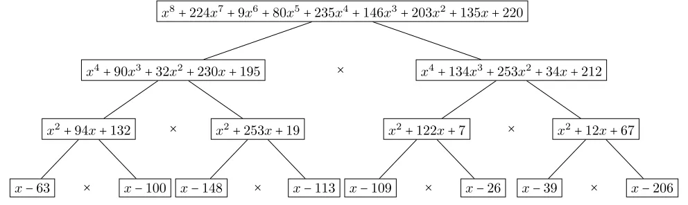
We want to evaluate it at the points (63,100,148,113,109,26,39,206).
The corresponding subproduct tree which will be constructed using a bottom-up
approach is illustrated in Figure 1.1.
x8+224x7+9x6+80x5+235x4+146x3+203x2+135x+220
x4+90x3+32x2+230x+195
x2+94x+132
x−63 x−100
x2+253x+19
x−148 x−113
x4+134x3+253x2+34x+212
x2+122x+7
x−109 x−26
x2+12x+67
x−39 x−206
× × × ×
× ×
×
Figure 1.1: Subproduct tree for evaluating a polynomials of degree 7 at 8 points.
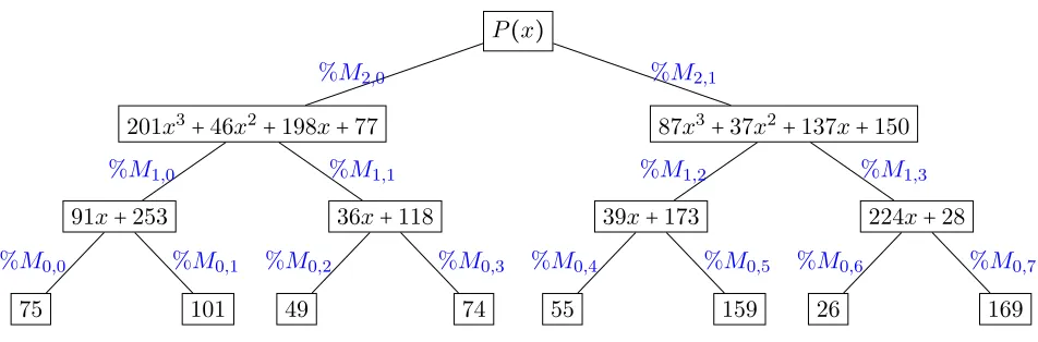
Then, we start the top-down approach for evaluating the polynomial in which, first, we need to compute the remainder of P(x)over two children of the root of the subproduct
tree, and evaluate each of the results at 4 points, and so on (do this recursively). In
Figure 1.2, this remaindering process is shown.
The final results of the remaindering process will be the evaluated results of the
polynomial at the given points over the prime field (257 in this case).
13
P(x)
201x3+46x2+198x+77
91x+253
75 %M0,0
101 %M0,1
%M1,0
36x+118
49 %M0,2
74 %M0,3
%M1,1
%M2,0
87x3+37x2+137x+150
39x+173
55 %M0,4
159 %M0,5
%M1,2
224x+28
26 %M0,6
169 %M0,7
%M1,3
%M2,1
Figure 1.2: Top-down remaindering process associated with the subproduct tree for eval-uating the example polynomial. The % symbol means mod operation. Mi,j is the j-th
Chapter 2
Background
In this chapter, we review basic concepts related to high performance computing. We
start with multi-core processors and the fork-join concurrency model. We continue with
the ideal cache model since cache complexity plays an important role for our algorithms
targeting multi-core processors. Then, we give an overview of GPGPU (general-purpose
computing on graphics processing units) followed by a model of computation devoted
to these many-core GPUs. We conclude this chapter by a presentation of FFT-based
algorithms, stated for vectors with coefficients in finite fields. Indeed, the algorithms of
Cooley-Tukey, Stockham, and Sch¨onhage & Strassen play an essential role in our work.
2.1
Multi-core processors
A multi-core processor is an integrated circuit consisting of two or more processors.
Having multiple processors would enhance the performance by giving the opportunity of executing tasks simultaneously. Ideally, the performance of a multi-core machine with
n processors, is n times that of a single processor (considering that they have the same frequency).
In recent years, this family of processors has become popular and widely being used
due to their performance and power consumption compared to single-core processors. In
addition, because of the physical limitations of increasing the frequency of processors,
or designing more complex integrated circuits, most of the recent improvements were in
designing multi-core systems.
In different topologies for multi-core systems, the cores may share the main memory,
cache, bus, etc. Plus, heterogeneous multi-cores may have different cores, however in
most cases the cores are similar to each others.
huge impact on the performance. Having cache memories on each of the processors, gives
the programmers an opportunity of designing extremely fast memory access procedures.
Implementing a program which can take benefits from the cache hierarchy, with low cache
misses rates is known to be challenging.
There are numerous parallel programming models based on these architectures. There
are some challenges whether in the programming models or in the application
develop-ment layers. For instance, how to divide and partition the task, how to make use of
cache and memory hierarchy, how to distribute and manage the tasks, how the tasks can
communicate with each-other, what is the memory access for each task. Some of these
worries will be handled in the concurrent programming platform, and some need to be
handled by the developer. Some well-known examples of these concurrent programming models areCilkPlus 1, OpenMP 2,MPI 3, etc.
2.1.1
Fork-join parallelism model
Fork-Join Parallelism Model is a multi-threading model for parallel computing. In this
model, execution of threaded programs is represented by DAG (directed acyclic graph)
in which the vertices correspond to threads, and edges (strands) correspond to relations
between threads (forked or Joined). Fork stands for ending one strand, and starting
a couple of new strands; whereas, join is the opposite operation in which a couple of
strands will end and one new strand begins.
1http://www.cilkplus.org/ 2http://openmp.org/wp/ 3
In the following diagram, a sampleDAG is shown
in which the program starts with the thread 1.
Later, the thread 2 will be forked to two threads
3 and 13. Following the the division of the
pro-gram, the threads 15, 17 and 12 will be joined to
18.
CilkPlus is a C++based platform providing an implementation of this model [43, 23, 19] using
work-stealing scheduling [3] in which every
pro-cessor has a stack of tasks, and all of the
proces-sors can steal tasks from others’ stacks when they
are idle. In CilkPlus extension, one can use the
keywordscilk spawnto fork, andcilk syncfor join.
According to theory analysis, this framework has
minimal overhead for tasks scheduling; this helps
the developers to exploit their applications to the
maximum parallelism.
1 start
2
3 13
4
6 14
16
5 7
9
8 10
11
12
15 17
18
For analyzing the parallelism in the fork-join model, we measure T1 and T∞ which
are defined as the following:
Work (T1): the total amount of time required to process all of the instructions of a
given program on a single-core machine.
Span (T∞): the total amount of time required to process all of the instructions of a given program on a multi-core machine with an infinite number of processors. This is called the critical path too.
Work/Span Law: the total amount of time required to process all of the instructions
of a given program using a multi-core machine with p processors (called Tp) is bounded
as the following:
Tp ≥ T∞ , Tp ≥
T1
p
Parallelism: the ratio of work tospan (T1/T∞).
In the above DAG the work, span, and the parallelism are 18, 9, and 2 respectively.
Greedy Scheduler A scheduler isgreedy if it attempts to do as much work as possible
at every step. In any greedy scheduler, there are two types of steps: complete steps
in which there are at least p strands that are ready to run (then the greedy scheduler selects any p of them and runs them), andincomplete step in which there are strictly fewer than pthreads that are ready to run (then the greedy scheduler runs them all).
Graham-Brent Theorem For any greedy scheduler, we have: Tp ≤ T1/p + T∞. Programming in Cilkplus
Here is an example of programming in Cilkplus for transposing a given matrix:
void transpose(T *A, int lda, T *B, int ldb, int i0, int i1, int j0, int j1){
tail:
int di = i1 - i0, dj = j1 - j0;
if (di >= dj && di > THRESHOLD) {
int im = (i0 + i1) / 2;
cilk_spawn transpose(A, lda, B, ldb, i0, im, j0, j1);
i0 = im; goto tail;
} else if (dj > THRESHOLD) {
int jm = (j0 + j1) / 2;
cilk_spawn transpose(A, lda, B, ldb, i0, i1, j0, jm);
j0 = jm; goto tail;
} else {
for (int i = i0; i < i1; ++i)
for (int j = j0; j < j1; ++j)
B[j * ldb + i] = A[i * lda + j];
}
}
In this implementation, we divide the problem into two subproblems based on the
in-put sizes. Then, the subproblems will be forked and executed in parallel. Note that when
the size of the problem is small enough, we execute the serial method; the THRESHOLD
would be decided based on the cache line size for which we make sure that the input and
f
athena,cel,prokop,sridhar
g@supertech.lcs.mit.edu
= ( )
( + = )
( +( = )( + )) ( )
( +( + + )= + =
p
)
( ; )
Q
cache
misses
organized by
optimal replacement
strategy
Main
Memory
Cache
Z
=L
Cache lines
Lines
of length
L
CPU
W
work
>
= ( );
( )
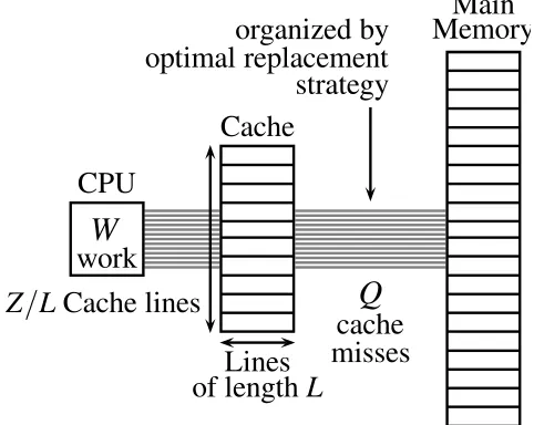
Figure 2.1: The ideal-cache model.
2.2
The ideal cache model
Thecache complexityof an algorithm aims at measuring the (negative) impact of memory
traffic between the cache and the main memory of a processor executing that algorithm.
Cache complexity is based on the ideal-cache model shown in Figure 2.1. This idea
was first introduced by Matteo Frigo, Charles E. Leiserson, Harald Prokop, and Sridhar
Ramachandran in 1999 [21]. In this model, there is a computer with a two-level memory hierarchy consisting of an ideal (data) cache of Z words and an arbitrarily large main memory. The cache is partitioned into Z/L cache lines where L is the length of each
cache line representing the amount of consecutive words that are always moved in a
group between the cache and the main memory. In order to achievespatial locality, cache
designers usually use L>1 which eventually mitigates the overhead of moving the cache
line from the main memory to the cache. As a result, it is generally assumed that the
cache is talland practically that we have
Z=Ω(L2).
In the sequel of this thesis, the above relation is referred as the tall cache assumption.
In the ideal-cache model, the processor can only refer to words that reside in the
cache. If the referenced line of a word is found in cache, then that word is delivered
to the processor for further processing. This situation is literally called a cache hit.
Otherwise, a cache miss occurs and the line is first fetched into anywhere in the cache
before transferring it to the processor; this mapping from memory to cache is calledfull
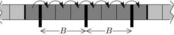
B
B
Figure 2.2: Scanning an array ofn=N elements, with L=B words per cache line. associativity. If the cache is full, a cache line must be evicted. The ideal cache uses the
optimal off-line cache replacement policy to perfectly exploit temporal locality. In this
policy, the cache line whose next access is furthest in the future is replaced [2].
Cache complexity analyzes algorithms in terms of two types of measurements. The
first one is the work complexity, W(n), where n is the input data size of the algorithm.
This complexity estimate is actually the conventional running time in a RAM model [1]. The second measurement is its cache complexity,Q(n;Z, L), representing the number of
cache misses the algorithm incurs as a function of:
• the input data size n,
• the cache size Z, and
• the cache line lengthL of the ideal cache.
When Z and L are clear from the context, the cache complexity can be denoted simply byQ(n).
An algorithm whose cache parameters can be tuned, either at compile-time or at
runtime, to optimize its cache complexity, is called cache aware; while other algorithms whose performance does not depend on cache parameters are calledcache oblivious. The
performance of cache-aware algorithm is often satisfactory. However, there are many
approaches which can be applied to design optimal cache oblivious algorithms to run on
any machine without fine tuning their parameters.
Although cache oblivious algorithms do not depend on cache parameters, their
anal-ysis naturally depends on the alignment of data block in memory. For instance, due
to a specific type of alignment issue based on the size of block and data elements (See
Proposition 1 and its proof), the cache-oblivious bound is an additive 1 away from the
external-memory bound [40]. However, such type of error is reasonable as our main goal is to match bounds within multiplicative constant factors.
Proposition 1 Scanning n elements stored in a contiguous segment of memory with cache line size L costs at most ⌈n/L⌉ +1 cache misses.
Proof. The main ingredient of the proof is based on the alignment of data elements
• Let (q, r) be the quotient and remainder in the integer division of n by L. Let u
(resp. w) be the total number of words in fully (not fully) used cache lines. Thus, we have n=u+w.
• Ifw=0 then(q, r) = (⌊n/L⌋,0)and the scanning costs exactlyq; thus the conclusion
is clear since ⌈n/L⌉ = ⌊n/L⌋in this case.
• If 0 < w < L then (q, r) = (⌊n/L⌋, w) and the scanning costs exactly q+2; the
conclusion is clear since⌈n/L⌉ = ⌊n/L⌋ +1 in this case.
• If L≤w<2Lthen (q, r) = (⌊n/L⌋, w−L) and the scanning costs exactly q+1; the
conclusion is clear again.
2.3
General-purpose computing on graphics
process-ing units
General-purpose computing on graphics processing units (GPGPU) is a way of doing
typical computations on Graphical processing units (GPU). The architecture of GPU,
has known to be suitable for some kind of computations in which one can achieve highly
efficient computing power compared to traditional ways of computing on CPU.
The architecture of a typical GPU, consists of streaming multiple-processors (SM)
which have multiple (8, typically) streaming processors which are SIMD (single
instruc-tion, multiple data) processors targeted for executing light threads. In a SM, there is
a shared memory which is accessible by each of the streaming processors. In addition,
each of the streaming processors have their own local registers. Each of the SMs will be
targeted for executing a block of threads.
There are two dominant platforms for programming GPUs: OpenCL 4 and CUDA 5
(from Nvidia). Here we investigate (and later use) CUDA.
2.3.1
CUDA
CUDA is a parallel programming architecture and model created by NVIDIA, which is a
C/C++ extension providing specific instruction sets for programming GPUs. It naively
supports multiple computational interfaces such as standard languages and APIs, but
having low overheads. It also provides accessing different hierarchy of the memory.
The CUDA programming model consists of the host which is a traditional CPU, and
one or more computing devices that are massively data-parallel co-processors (GPUs).
4http://www.khronos.org/opencl/
Figure 2.3: Illustration of the CUDA memory hierarchy [56]
Each device is equipped with a large number of arithmetic execution units that has its
own DRAM, and runs many threads in parallel.
To invoke calculations on the GPU one has to perform a kernel launch, which is
basically a function written with the intent of what each thread on the GPU is to perform.
The GPU has a specific architecture of threads where they are divided into blocks and
where blocks are divided into a grid, see Figure 2.3. The grid has two dimensions and
can contain up to 65536 blocks in each dimension. While each block contains threads
in three dimensions, and can contain up to 512 threads in two dimensions and 64 in the
third. When executing a kernel one specifies the dimensions of the grid and blocks to specify how many threads will be executing the kernel.
GPU has its own DRAM which is used in communicating with the host system. To
accelerate calculations within the GPU itself there are several other layers of memory
such as constant, shared and texture. Table 2.1 shows the relation between these.
Programming in CUDA
Here is an example of programming in CUDA for transposing of a given matrix:
Memory Location Cached Access Scope in Architecture
Register On-chip No Read/Write Single thread Local Off-chip No Read/Write Single thread Shared On-chip No Read/Write Threads in a Block Global On-chip No Read/Write All
Constant On-chip Yes Read All Texture On-chip Yes Read All
Table 2.1: Table showing CUDA memory hierarchy [56]
__shared__ float tile[TILE_DIM][TILE_DIM];
int xIndex = blockIdx.x * TILE_DIM + threadIdx.x;
int yIndex = blockIdx.y * TILE_DIM + threadIdx.y;
int index_in = xIndex + yIndex * width;
xIndex = blockIdx.y * TILE_DIM + threadIdx.x;
yIndex = blockIdx.x * TILE_DIM + threadIdx.y;
int index_out = xIndex + yIndex * height;
for (int i = 0; i < TILE_DIM; i += BLOCK_ROWS) {
tile[threadIdx.y + i][threadIdx.x] = idata[index_in + i*width];
}
__syncthreads();
for (int i = 0; i < TILE_DIM; i += BLOCK_ROWS) {
odata[index_out + i*height] = tile[threadIdx.x][threadIdx.y + i];
}
}
The global identifies that this function is a kernel which means it will be executed
on the GPU. The host will invoke this kernel by specifying the number of thread blocks,
and number of threads per block. Then, each of the threads will execute this function
having access to the shared memory allocated on the thread block and the global memory.
Note that each thread has different id (see threadIdx.x and threadIdx.y), as each thread
block has different id (see blockIdx.x and blockIdx.y).
In this implementation, tile is the allocated memory on the shared memory. Then,
memory. After synchronizing, which means to make sure that all of the memory-reading
are completed, we copy the elements of the transposed matrix from the shared memory
to the correct index in the global memory. So, each of the thread blocks are responsible
for transposing a tile of the matrix.
2.4
Many-core machine model
Many-core Machine Model (MMM) is a model of multi-threaded computation, combining
fork-join and single-instruction-multiple-data parallelisms, with an emphasis on
estimat-ing parallelism overheads of programs written for modern many-core architectures [35]. Using this model, one can minimize parallelism overheads by determining an appropriate
value range for a given program parameter.
Architecture An MMM abstract machine has a similar architecture as a GPU in which
we have infinite and identical number of streaming multiprocessors. Each of the SM has
a finite number of processing cores and a fixed-size local memory. Plus, it has 2-level
memory hierarchy: one unbounded global memory with high latency and low throughput,
and SM local memory having low latency and high throughput.
Program An MMM program is a directed acyclic graph (DAG) whose vertices are
kernels and where edges indicate dependencies. A kernel is a SIMD (single instruction
multi-threaded data) program decomposed into a number of blocks. Each
thread-block is executed by a single SM and each SM executes a single thread-thread-block at a time.
Scheduling and synchronization At run time, an MMM machine schedules thread-blocks onto the SMs, based on the dependencies among kernels and the hardware
re-sources required by each thread-block. Threads within a thread-block cooperate with
each other via the local memory of the SM running the thread-block. Thread-blocks
interact with each other via the global memory
Memory access policy All threads of a given thread-block can access simultaneously
any memory cell of the local memory or the global memory. Read/Write conflicts are
handled by the CREW (concurrent read exclusive write) policy.
For the purpose of analyzing program performance, we define two machine
• U: Time (expressed in clock cycles) spent for transferring one machine word be-tween the global memory and the local memory of any SM (so-called shared
mem-ory).
• Z: Size (expressed in machine words) of the local memory of SM.
Kernel DAG Each MMM program P is modeled by a directed acyclic graph (K, e) ,
called the kernelDAGofP, where each node represents a kernel, and each edge represents a kernel call which must precede another kernel call. (a kernel call can be executed
whenever all its predecessors in theDAG completed their execution)
Since each kernel of the programP decomposes into a finite number of thread-blocks, we mapP to a second graph, called thethread blockDAGofP, whose vertex setB(P)
consists of all thread-blocks of the kernels of P, such that (B1, B2) is an edge if B1 is a
thread-block of a kernel preceding the kernel of B2 inP.
2.4.1
Complexity measures
Work The work of a thread-block is defined as the total number of local operations
performed by the threads in that block. The work of a kernel k is defined as the sum of the works of its thread-blocks (W(k)). The work of an entire program P is defined as
W(P)which is defined as the total work of all its kernels:
W(P) = ∑
k∈K
W(k)
Span The span of a thread-block is defined as the maximum number of local operations
performed by the threads in that block. The span of a kernelk is defined as the maximum span of its thread-blocks (S(k)). The span of the path γ if defined as the sum of the
span of all kernels in that path: S(γ) = ∑k∈γS(k)
The span of an entire program P is defined as:
S(P) =max
γ S(γ)
Overhead The overhead of a thread-blockBis defined as(r+w)U, assuming that each
total overhead of all its kernels:
O(P) = ∑
α
O(α)
Graham-Brent Theorem for MMM We have the following estimate for the running
time Tρ of the program ρ when executing it on p Streaming Multiprocessors:
Tp≤ (N(ρ)/p+L(ρ)) . C(ρ)
where N(ρ)is the number of vertices in the thread-block DAG of ρ, L(ρ) is the critical
path length (the length of the longest path) in the thread-block DAG of ρ, and C(ρ) =
maxB′ ∈B(ρ)(S(B′) +O(B′)).
2.5
Fast Fourier transform over finite fields
Most multiplication algorithm such as Karatsuba, Toom-Cook, and FFT use
evaluation-interpolation approach. The fast Fourier transform (FFT) is also based on this approach
in which the evaluation and interpolation are done on specific points (roots of unity)
which is relatively efficient compared to its counterparts.
Definition let R be a ring, and K ≥2∈N, and ω be the Kth root of unity in R; this
means that ωK = 1 and
∑Kj=−01ωij =0 for 1 ≤i <K. The Fourier transform of a vector
A= [A0, . . . , AK−1] fromR is ˆA= [Aˆ0, . . . ,AKˆ−1]where for 0≤i<K: ˆAi = ∑jK=−01wijAj.
Fourier transform computing ˆAin the naive way, takesO(K2), but usingfast Fourier transform which is a divide & conquer algorithm, it takesO(KlogK).
Inverse Fourier transform is the reverse operation ofFourier transform which com-putes the vector A by having ˆA as an input. The complexity of this operation is also
O(KlogK). It can be proven that the inverse transform is the same operation as the
transform, but the points of the vector are shuffled.
Multiplication given input polynomialsfandgof degreeKdefined asf(x) = ∑Ki=0fixi
and g(x) = ∑Ki=0gixi.
1. Say ω is the 2Kth root of unity. Then, we evaluate both polynomials at points
defined above. This step is called Discrete Fourier Transform.
2. Point-wise multiplication: (f(ω0).g(ω0), . . . , f(ω2K−1).g(ω2K−1)).
3. Interpolating the result polynomial using inverse Fourier transform.
The overall cost of multiplication using FFT algorithm is O(KlogK).
2.5.1
Sch¨
onhage-Strassen FFT
The Sch¨onhage-Strassen [58] FFT algorithm which is known to be asymptotically the
best multiplication algorithm with complexity O(nlognlog logn) (until F¨urer’s
algo-rithm [24]) works on the ring Z/(2n+1)Z. Algorithm 1 (this algorithm is from [8,
Section 2.3]) is the Sch¨onhage-Strassen approach for multiplying two integers having
at-mostn bits. Note that in the Algorithm 1, if the chosenn′is large, we call the algorithm recursively.
Algorithm 1: Sch¨onhageStrassen
Input: 0≤A, B<2n+1,K =2k, n=M K Output: C =A.B mod(2n+1)
A= ∑Kj=−01aj2j M
, B= ∑Kj=−01bj2j M
where 0≤aj, bj <2M;
choose n′≥2n/K+k which is multiple of K;
θ=2n ′/K
, ω =θ2; for j=0. . . k−1 do
aj =θjaj mod(2n ′
+1);
bj =θjbj mod(2n ′
+1);
a=FFT(a, ω, K);
b=FFT(b, ω, K); for j=0. . . k−1 do
cj =ajbj mod(2n ′
+1);
c=InverseFFT(c, ω, K); for j=0. . . k−1 do
cj =cj/(Kθj) mod(2n ′
+1); if cj ≥ (j+1)22M then
cj =cj− (2n ′
+1);
C = ∑Kj=−01cj2j M
;
2.5.2
Cooley-Tukey and Stockham FFT
This section reviews the Fast Fourier Transform (FFT) in the language of tensorial
cal-culus, see [45] for an extensive presentation. Throughout this section, we denote byK a
field. In practice, this field is often a prime fieldZ/pZwherepis a prime number greater
than 2.
Basic operations on matrices
Let n, m, q, s be positive integers and let A, B be two matrices over K with respective dimensions m×n and q×s. The tensor (or Kronecker) product of A byB is an mq×ns
matrix over Kdenoted by A⊗B and defined by
A⊗B= [ak`B]k,` with A= [ak`]k,` (2.1)
For example, let
A= ⎡ ⎢ ⎢ ⎢ ⎢ ⎣ 0 1 2 3 ⎤ ⎥ ⎥ ⎥ ⎥ ⎦
and B = ⎡ ⎢ ⎢ ⎢ ⎢ ⎣ 1 1 1 1 ⎤ ⎥ ⎥ ⎥ ⎥ ⎦ . (2.2)
Then their tensor products are
A⊗B= ⎡ ⎢ ⎢ ⎢ ⎢ ⎢ ⎢ ⎢ ⎢ ⎢ ⎣
0 0 1 1
0 0 1 1
2 2 3 3
2 2 3 3
⎤ ⎥ ⎥ ⎥ ⎥ ⎥ ⎥ ⎥ ⎥ ⎥ ⎦
and B⊗A= ⎡ ⎢ ⎢ ⎢ ⎢ ⎢ ⎢ ⎢ ⎢ ⎢ ⎣
0 1 0 1
2 3 2 3
0 1 0 1
2 3 2 3
⎤ ⎥ ⎥ ⎥ ⎥ ⎥ ⎥ ⎥ ⎥ ⎥ ⎦ . (2.3)
Denoting by In the identity matrix of order n, we emphasize two particular types of
tensor products, In⊗Am and An⊗Im, where Am (resp. An) is a square matrix of order
m (resp, n) over K.
I4⊗DFT2 = ⎡ ⎢ ⎢ ⎢ ⎢ ⎢ ⎢ ⎢ ⎢ ⎢ ⎢ ⎢ ⎢ ⎢ ⎢ ⎢ ⎢ ⎢ ⎢ ⎢ ⎢ ⎢ ⎣ 1 1
1 −1
1 1 1 −1
1 1
1 −1
1 1
1 −1 ⎤ ⎥ ⎥ ⎥ ⎥ ⎥ ⎥ ⎥ ⎥ ⎥ ⎥ ⎥ ⎥ ⎥ ⎥ ⎥ ⎥ ⎥ ⎥ ⎥ ⎥ ⎥ ⎦
DFT2⊗I4 = ⎡ ⎢ ⎢ ⎢ ⎢ ⎢ ⎢ ⎢ ⎢ ⎢ ⎢ ⎢ ⎢ ⎢ ⎢ ⎢ ⎢ ⎢ ⎢ ⎢ ⎢ ⎢ ⎣ 1 1 1 1 1 1 1 1 1 1 1 1 −1 −1 −1 −1 ⎤ ⎥ ⎥ ⎥ ⎥ ⎥ ⎥ ⎥ ⎥ ⎥ ⎥ ⎥ ⎥ ⎥ ⎥ ⎥ ⎥ ⎥ ⎥ ⎥ ⎥ ⎥ ⎦
The direct sum of A and B is an (m+q) × (n+s) matrix over K denoted by A⊕B
and defined by
A⊕B = ⎡ ⎢ ⎢ ⎢ ⎢ ⎣ A 0 0 B ⎤ ⎥ ⎥ ⎥ ⎥ ⎦ . (2.4)
More generally, for n matrices A0, . . . , An−1 over K, the direct sum of A0, . . . , An−1 is
defined as ⊕ni=−01Ai = A0 ⊕ (A1 ⊕ (⋯ ⊕An−1)⋯). The stride permutation matrix Lmnm
permutes an input vector x of lengthmn as follows
x[im+j] ↦x[jn+i], (2.5)
for all 0 ≤ j < m, 0 ≤ i < n. If x is viewed as an n×m matrix, then Lmnm performs a
transposition of this matrix.
Discrete Fourier transform
We fix an integer n≥2 and an n-th primitive root of unity ω∈K. The n-point Discrete
Fourier Transform (DFT) at ω is a linear map from the K-vector space Kn to itself,
defined by x z→DFTnx with the n-th DFT matrix
DFTn= [ωk`]0≤k, `<n. (2.6)
In particular, the DFT of size 2 corresponds to the butterfly matrix
DFT2 = ⎡ ⎢ ⎢ ⎢ ⎢ ⎣ 1 1
1 −1 ⎤ ⎥ ⎥ ⎥ ⎥ ⎦ . (2.7)
The well-known Cooley-Tukey Fast Fourier Transform (FFT) [14] in its recursive form
DFTn, for any integers q, s such thatn=qs holds:
DFTqs= (DFTq⊗Is)Dq,s(Iq⊗DFTs)Lqsq , (2.8)
where Dq,s is the diagonal twiddle matrix defined as
Dq,s=
q−1 ⊕
j=0
diag(1, ωj, . . . , ωj(s−1)), (2.9)
Formula (2.10) illustrates Formula (2.8) with DFT4:
DFT4 = (DFT2⊗I2)D2,2(I2⊗DFT2)L22
= ⎡ ⎢ ⎢ ⎢ ⎢ ⎢ ⎢ ⎢ ⎢ ⎢ ⎣
1 0 1 0
0 1 0 1 1 0 −1 0
0 1 0 −1 ⎤ ⎥ ⎥ ⎥ ⎥ ⎥ ⎥ ⎥ ⎥ ⎥ ⎦ ⎡ ⎢ ⎢ ⎢ ⎢ ⎢ ⎢ ⎢ ⎢ ⎢ ⎣
1 0 0 0
0 1 0 0 0 0 1 0
0 0 0 ω
⎤ ⎥ ⎥ ⎥ ⎥ ⎥ ⎥ ⎥ ⎥ ⎥ ⎦ ⎡ ⎢ ⎢ ⎢ ⎢ ⎢ ⎢ ⎢ ⎢ ⎢ ⎣
1 1 0 0
1 −1 0 0
0 0 1 1
0 0 1 −1 ⎤ ⎥ ⎥ ⎥ ⎥ ⎥ ⎥ ⎥ ⎥ ⎥ ⎦ ⎡ ⎢ ⎢ ⎢ ⎢ ⎢ ⎢ ⎢ ⎢ ⎢ ⎣
1 0 0 0
0 0 1 0 0 1 0 0
0 0 0 1
⎤ ⎥ ⎥ ⎥ ⎥ ⎥ ⎥ ⎥ ⎥ ⎥ ⎦ = ⎡ ⎢ ⎢ ⎢ ⎢ ⎢ ⎢ ⎢ ⎢ ⎢ ⎣
1 1 1 1
1 ω −1 −ω
1 −1 1 −1
1 −ω −1 ω ⎤ ⎥ ⎥ ⎥ ⎥ ⎥ ⎥ ⎥ ⎥ ⎥ ⎦ = ⎡ ⎢ ⎢ ⎢ ⎢ ⎢ ⎢ ⎢ ⎢ ⎢ ⎣
1 1 1 1
1 ω1 ω2 ω3
1 ω2 ω4 ω6
1 ω3 ω6 ω9 ⎤ ⎥ ⎥ ⎥ ⎥ ⎥ ⎥ ⎥ ⎥ ⎥ ⎦ . (2.10)
Assume that n is a power of 2, say n =2k. Formula (2.8) can be unrolled so as to
reduce DFTn to DFT2 (or a base case DFTm, where m divides n) together with the
appropriate diagonal twiddle matrices and stride permutation matrices. This unrolling
can be done in various ways. Before presenting one of them, we introduce a notation.
For integersi, j, h≥1, we define
∆(i, j, h) = (Ii⊗DFTj⊗Ih) (2.11)
which is a square matrix of size ijh. For m = 2` with 1≤ ` < k, the following formula
holds:
DFT2k = (
k−`
∏
i=1
∆(2i−1,2,2k−i) (I2i−1⊗D2,2k−i))∆(2k−`, m,1) ( 1 ∏
i=k−`
(I2i−1⊗L 2k−i+1
2 )).
(2.12)
Therefore, Formula (2.12) reduces the computation of DFT2k to composing DFT2, DFT2`,
factoriza-tion of the matrix DFT2k is
DFT2k = (DFT2⊗I2k−1)D2,2k−1L2
k
2 (DFT2k−1⊗I2), (2.13)
from which one can derive the Stockham FFT [59] as follows
DFT2k =
k−1 ∏
i=0
(DFT2⊗I2k−1)(D2,2k−i−1 ⊗I2i)(L2
k−i
2 ⊗I2i). (2.14)
This is a basic routine which is implemented in our library (CUMODP 6) as the FFT
over a finite field (prime) targeted GPUs [53].
6
Chapter 3
Parallelizing classical algorithms for
dense integer polynomial
multiplication
For a given algorithmic problem, such as performing dense polynomial multiplication over
a given coefficient ring, there are at least two natural approaches for obtaining an efficient
parallel solution. The first one is to start from a good serial solution and parallelize it, if
possible. The second one is to start from a good parallel solution of a related algorithmic
problem and transform it into a good parallel solution of the targeted problem.
In this chapter, for the question of performing dense polynomial multiplication over
the integers, we follow the first approach, reserving the second one for the next chapter.
To be more specific, we consider below standard sequential algorithms and discuss their
parallelization in CilkPlustargeting multi-core systems.
Interpreting experimental performance results of a parallel program is often a
chal-lenge, since many phenomena may interfere with each other: the underlying algorithm,
its implementation, issues related to the hardware or to the concurrency platform
exe-cuting the program. Complexity estimates of the underlying algorithms can help with
this interpretation. However, it is essential not to limit algorithm analysis to arithmetic
count. To this end, we review those algorithms and analyze their algebraic complexity
in Sections 3.2 through 3.4. Then, we discuss their parallelization and analyze the cor-responding complexity measures in Section 3.5. Experimental results are reported and
analyzed in Section 3.6.
3.1
Preliminary results
Notation 1 We consider two polynomials f, g ∈Z[x] written as follows:
f(x) =
m−1
∑
i=0
fixi , g(x) = n−1
∑
i=0
gixi (3.1)
where n, m∈N>0 and, for 0≤i<m and 0≤j <n, we have fi , gj ∈ Z together with ∣fi∣ ≤2bf and∣gj∣ ≤2bg, for some bf, bg ∈N. We want to compute the polynomial h∈Z[x] defined by:
h(x) =
n+m−2
∑
i=0
hixi =f(x) ×g(x). (3.2) Algorithm 2: Schoolbook(f, g, m, n)
Input: f, g∈Z[x] and m, n∈N>0 as in Notation 1. Output: h∈Z[x] such that h=f.g.
for i=0. . . m−1do for j=0. . . n−1 do
hi+j =hi+j+fi . gj;
return h;
One naive solution for computing the product h is the so-called schoolbook method
(Algorithm 2) which requires O(nm) arithmetic operation on the coefficients. If the
coefficients are all of small size in comparison to n andm, then this upper bound can be regarded as a running time estimate, in particular if the coefficients are of machine word
size. However, if the coefficients are large, it becomes necessary to take their size into
account when estimating the running time of Algorithm 2. This explains the introduction
of Assumption 1.
This phenomenon occurs frequently with the univariate polynomials resulting from
solving multivariate polynomials systems of equations and inequalities. In such case, the
resulting univariate polynomials are often dense in the sense that the bit size of each
coefficient is the same order of magnitude as the degree, thus implying bf ∈Θ(n).
For us, these polynomials are of great interest since isolating their real roots is a key
step in the process of solving polynomials systems. At the same time, the size of these
coefficients makes real root isolation an extremely expensive task in terms of computing resources, leading to the use of high-performance computing techniques, such as parallel
Assumption 1 The implementation of all the algorithms studied in this work relies on
the GNU Multi-Precision (GMP) library 1. The purpose of Proposition 2 is to give an
asymptotic upper bound for GMP’s integer multiplication. We will use this estimate in the
analysis of our algorithms for dense polynomial multiplication with integer coefficients.
Proposition 2 Multiplying two integersX andY, withbX andbY bits, amounts at most
to Cmul(bX+bY)log(bX+bY)log(log(bX+bY)) bit operations, for some constant Cmul (that we shall use in our later estimates).
Proof. The GMP library relies on different algorithms for multiplying integers [32].
For the largest input sizes, the FFT-based Sch¨onhage and Strassen algorithms (SSA) is
used. These sizes are often reached in the implementation of our algorithms for dense
polynomial multiplication with integer coefficients. The bit complexity for SSA to
mul-tiply two integers with a N-bit result is O(N logN log logN) [32, Chapter 16]. The
conclusion follows from the fact that the product X×Y has N =bX +bY bits. ◻ Proposition 3 Multiplying two integers X and Y, with bX and bY bits, assuming Y of
machine word size, amounts at most to Cmul′ bX bit operations, for some constant Cmul′
(that we shall use in our later estimates).
Proof. Indeed, under the assumption that Y is of machine word size, the GMP
library relies on schoolbook multiplication [32]. The conclusion follows. Note that Cmul′
depends on the machine word size. ◻
Remark 1 In Proposition 2, the cost is calculated in bit operations. In other
circum-stances, counting machine-word operations will be more convenient. For us, the bit size
of a machine word is a “small” constant, denoted by MW, which, in practice is either 32
or 64 bits. Hence, we will state our algebraic cost estimates either in bit operations or in machine-word operations, whichever works best in the context of the estimate,
Notation 2 For all real number X≥2, we define
G(X) =CmulX logXlog logX.
Consequently, the estimate stated in Proposition 2 becomes G(bX +bY).
Remark 2 The algebraic complexity of adding two integers, each of at most h bits, is at most Caddh, for some constant Cadd (that we shall use in our later estimates).
Proposition 4 Addingp≥2integers, each of at mosthbits, amounts at most to Caddh p bit operations.
Proof. Up to adding zero items in the input, we can freely assume thatpis a power
of 2. At first, we are adding p/2 pairs of integers having at most h bits which produce
p/2 integers having at mosth+1 bits. Then we will havep/4 pairs of integers which their
results will haveh+2 bits. By continuing in this manner and using Remark 2 we have:
Cadd (p2h+2p2 (h+1) + ⋯ +
p
2log2p(h+log2p−1)) = Cadd(p h∑logi=12p 21i +p∑
log2p
i=1
i−1 2i )
= Cadd(p h(2log2
p−1
2log2p ) +h(
2log2p−log2p−2
2log2p ))
= Cadd(p h(p−p1) +h (p−logp2p−2)) = Cadd(h(p−1) +h(1−log2pp+2)) ≤ Cadd(h(p−1) +h)
= Caddp h
◻
Assumption 2 For simplicity, we assume that m≤n holds in all subsequent results. Proposition 5 The number of bit operations performed by Algorithm 2 is at most:
m nG(bf+bg) +Caddm n(bf +bg)
Proof. We havem×nmultiplications of two integers with maximum sizesbx andby,
respectively. Using Proposition 2, this gives us the first term of the desired complexity estimate. For the additions, assuming that m ≤ n holds, we need to add m integers
with the maximum size of bx +by in order to obtain the coefficient of xi in f ×g, for
m−1≤i≤n−1. For 0≤i<m−1, the coefficient of xi requires addingi+1 integers with
bx+by bits. Similarly, forn≤i≤m+n−2, the degree ofxi requires adding(n+m−2) −i+1
integers with bx+by bits. Therefore, the total cost for the additions sums up to:
Cadd (m((n−1) − (m−1) +1) +2
m−2
∑
i=0
(i+1)) (bx+by) =Caddm n(bx+by)
◻
Assumption 3 For the purpose of our application to real root isolation, we shall assume
polynomial is of the same order as the degree of that polynomial. This implies that, for
all 0≤i<n, we have ∣fi∣ ∈Θ(2n) and ∣gi∣ ∈Θ(2n).
Corollary 1 Under Assumption 3, the complexity estimate of Algorithm 2 becomes
2Cmuln3 log(2n)log log(2n) +2Caddn3.
3.2
Kronecker substitution method
In this section, we investigate an algorithm for doing polynomial multiplication which
takes advantage of integer multiplications. For this purpose, we convert polynomials to
relatively large integers, do the integer multiplication, then convert back the result into
a polynomial. This method is an application of the so-called Kronecker substitution,
see [29, Section 8.3] and [18].
As in Section 3.1, we assume that f and g are univariate polynomials over Z with variable x and with respective positive degrees m and n, see Notation 1. Furthermore, we start by assuming that all of the coefficients of f and g are non-negative. The case of negative coefficients is handled in Section 3.2.1.
With this latter assumption, we observe that every coefficient in the productf(x)⋅g(x)
is strictly bounded over by H=min(m, n)HfHg+1 where Hf and Hg are the maximum
value of the coefficients in f and g, respectively. Recall that the binary expansion of a positive integer A has exactly b(A) = ⌊log2(A)⌋ +1 bits. Thus, every coefficient of f, g,
and f⋅g can be encoded with at most β bits, whereβ =b(H).
Here are the steps of Kronecker substitution for doing integer polynomial
multiplica-tion:
1. Convert-in: we respectively map the input polynomials f(x) and g(x) to the
integers Zf and Zg defined as:
Zf = ∑ 0≤i<m
fi2β i and Zg = ∑ 0≤i<n
gi2β i. (3.3)
2. Multiplying: multiply Zf and Zg: Zf g =Zf . Zg.
3. Convert-out: retrieve coefficients of the product (f.g) from Zf g.
One can regard 2β as a variable, and thus, Z
f and Zg are polynomials in Z[2β]. By
definition of H, each coefficient of Zf ⋅Zg (computed in Z[2β]) is in the range [0, H).
the product Zf g of Zf and Zg as an integer number and retrieve the coefficients of the
polynomialf⋅g from the binary expansion ofZf g. This trick allows us to take advantage
of asymptotically fast algorithms for multi-precision integers, such as those implemented
in the GMP-library.
3.2.1
Handling negative coefficients
We apply a trick which was proposed by R. Fateman [18] in which for each of the
neg-ative coefficients (starting from the least significant one), 2β is borrowed from the next
coefficient. For instance, assuming
f(x) =f0+ ⋯ +fixi+fi+1xi+1+ ⋯ +fdxd (3.4)
where fi <0 holds, we replace f(x) by
f0+ ⋯ + (2β−fi)xi+ (fi+1−1)xi+1+ ⋯ +fdxd. (3.5)
There’s only one special case to his procedure: when the leading coefficient itself is
negative. In this situation, the polynomial f(x) is replaced by −f(x) and Zf g by −Zf g.
Since Fateman’s trick may increment each coefficient of f or g by 1, it is necessary to replace β by β′=β+1 in the above algorithm.
For the Convert-outstep, if the most significant bit of a 2β′
-digit is 1, then it
repre-sents a negative coefficient and it should be adjusted by subtracting from 2β′
. Otherwise,
it is a positive coefficient, and no adjustment is required. Algorithm 3 below sketches
integer polynomial via Kronecker substitution.
Algorithm 3: KroneckerSubstitution(f, g, m, n)
Input: f, g∈Z[x] and m, n∈N are the sizes respectively. Output: h∈Z[x] such that h=f.g.
β = DetermineResultBits(f, g, m, n);
Zf =ConvertToInteger(f, m, β);
Zg =ConvertToInteger(g, n, β);
Zf g =Zf ×Zg;
h=ConvertFromInteger(Zf g, β, m+n−1);
return h;
![Figure 2.3: Illustration of the CUDA memory hierarchy [56]](https://thumb-us.123doks.com/thumbv2/123dok_us/7776421.1282563/27.612.93.537.70.357/figure-illustration-cuda-memory-hierarchy.webp)
![Table 2.1: Table showing CUDA memory hierarchy [56]](https://thumb-us.123doks.com/thumbv2/123dok_us/7776421.1282563/28.612.119.513.71.177/table-table-showing-cuda-memory-hierarchy.webp)