Performance Analysis of Effective Symbolic Methods for Solving Band Matrix SLAEs

(1)

Performance Analysis of Effective Symbolic Methods for

Solving Band Matrix SLAEs

MilenaVeneva1,∗_and _Alexander_Ayriyan1,∗∗

1_{Joint Institute for Nuclear Research, Laboratory of Information Technologies, Joliot-Curie 6, 141980} Dubna, Moscow region, Russia

Abstract. This paper presents an experimental performance study of imple-mentations of three symbolic algorithms for solving band matrix systems of linear algebraic equations with heptadiagonal, pentadiagonal, and tridiagonal coefficient matrices. The only assumption on the coefficient matrix in order for the algorithms to be stable is nonsingularity. These algorithms are implemented using theGiNaClibrary ofC++and theSymPylibrary ofPython, considering five different data storing classes. Performance analysis of the implementations is done using the high-performance computing (HPC) platforms “HybriLIT” and “Avitohol”. The experimental setup and the results from the conducted computations on the individual computer systems are presented and discussed. An analysis of the three algorithms is performed.

1 Introduction

Systems of linear algebraic equations (SLAEs) with heptadiagonal (HD), pentadiagonal (PD) and tridiagonal (TD) coefficient matrices may arise after many different scientific and engi-neering problems, as well as problems of the computational linear algebra where finding the solution of a SLAE is considered to be one of the most important problems. On the other hand, special matrix’s characteristics like diagonal dominance, positive definiteness, etc. are not always feasible. The latter two points explain why there is a need of methods for solving of SLAEs which take into account the band structure of the matrices and do not have any other special requirements to them. One possible approach to this problem is the symbolic algorithms. An overview of some of the symbolic algorithms which exist in the literature is done by us in [1]. What is common for all of them, is that they are implemented using Computer Algebra Systems (CASs) such asMaple,Mathematica, andMatlab.

Three direct symbolic algorithms for solving a SLAE based on LU decomposition are considered: for HD matrices (see [2] and [1]) –SHDM, for PD [3] –SPDM, and TD matri-ces [4] –STDM. The only assumption on the coefficient matrix is nonsingularity.

The choice of algorithms for solving problems of the computational linear algebra is cru-cial for the programs’ effectiveness, especru-cially when these problems are with a big dimension. In that case they require the use of supercomputers and computer clusters for the solution to be obtained in a reasonable amount of time. Another important choice that has to be made and that influences the programs’ performance is what programming language to be used for

(2)

the algorithms’ implementations. Here, we are going to focus on two of the most popular pro-gramming languages for scientific computations, namelyC++andPython. The aim of this paper, which is a logical continuation of [5] and [6], is to investigate the performance charac-teristics of the considered serial methods with their two implementations being executed on modern computer clusters.

2 Computational Experiments

Computations were held on the basis of the heterogeneous computational platform “Hy-briLIT” (1142 TFlops/s for single precision and 550 TFlops/s for double precision) [7] at the Laboratory of Information Technologies of the Joint Institute for Nuclear Research in the town of science Dubna, Russia, and on the cluster computer system “Avitohol” (412.3 TFlops/s for double precision) [8] at the Advanced Computing and Data Centre of the Institute of Information and Communication Technologies of the Bulgarian Academy of Sciences in Sofia, Bulgaria. The latter has been ranked among the TOP500 list (https: //www.top500.org) twice – being 332nd in June 2015 and 388th in November 2015.

2.1 Experimental Setup

Table 1 sums up some basic information about hardware on the two computer systems, includ-ing models of processors, processors’ base frequency, and amount of cache memory (Smart-Cache). For even more information, visit: https://ark.intel.com/compare/75281,75269. Ta-ble 2 summarizes the basic information about the compilers and libraries used on the two computer systems. The three algorithms are implemented using the GiNaC library [9] of C++[10] (the projects are built with the help of CMake [11]), and SymPy [12] library of Python[13] (using Anaconda distribution [14]). The reason why optimization -O0 was used is that theGiNaClibrary is already optimized and any further attempts to optimize the code give worse results. Although we use Py 2.7, one should note that the implementations are fully compatible with Py 3.6 as well. It is worth mentioning that optimization attempts like autowrapandnumbado not give better execution times. The former because of overhead, the second one because it cannot optimize further than what is already done.

Table 1:Intel processors used for numerical experiments.

Computer system Processor FREQ [GHz] Cache [MB]

“HybriLIT” Intel Xeon E5-2695v2 2.40 30

“Avitohol” Intel Xeon E5-2650v2 2.60 20

2.2 Experimental Results and Analysis of the Algorithms

(3)

the algorithms’ implementations. Here, we are going to focus on two of the most popular pro-gramming languages for scientific computations, namelyC++andPython. The aim of this paper, which is a logical continuation of [5] and [6], is to investigate the performance charac-teristics of the considered serial methods with their two implementations being executed on modern computer clusters.

2 Computational Experiments

Computations were held on the basis of the heterogeneous computational platform “Hy-briLIT” (1142 TFlops/s for single precision and 550 TFlops/s for double precision) [7] at the Laboratory of Information Technologies of the Joint Institute for Nuclear Research in the town of science Dubna, Russia, and on the cluster computer system “Avitohol” (412.3 TFlops/s for double precision) [8] at the Advanced Computing and Data Centre of the Institute of Information and Communication Technologies of the Bulgarian Academy of Sciences in Sofia, Bulgaria. The latter has been ranked among the TOP500 list (https: //www.top500.org) twice – being 332nd in June 2015 and 388th in November 2015.

2.1 Experimental Setup

Table 1 sums up some basic information about hardware on the two computer systems, includ-ing models of processors, processors’ base frequency, and amount of cache memory (Smart-Cache). For even more information, visit: https://ark.intel.com/compare/75281,75269. Ta-ble 2 summarizes the basic information about the compilers and libraries used on the two computer systems. The three algorithms are implemented using the GiNaC library [9] of C++ [10] (the projects are built with the help of CMake [11]), andSymPy [12] library of Python[13] (using Anaconda distribution [14]). The reason why optimization -O0 was used is that theGiNaClibrary is already optimized and any further attempts to optimize the code give worse results. Although we use Py 2.7, one should note that the implementations are fully compatible with Py 3.6 as well. It is worth mentioning that optimization attempts like autowrapandnumbado not give better execution times. The former because of overhead, the second one because it cannot optimize further than what is already done.

Table 1:Intel processors used for numerical experiments.

Computer system Processor FREQ [GHz] Cache [MB]

“HybriLIT” Intel Xeon E5-2695v2 2.40 30

“Avitohol” Intel Xeon E5-2650v2 2.60 20

2.2 Experimental Results and Analysis of the Algorithms

During our experiments wall-clock times were collected and the average time from mul-tiple runs is reported. For that purpose, we use the function now() of the class std::chrono::high_resolution_clockforC++(requires at least standardc++11), and timeit.default_timer()forPython. Both of them provide the best clock rate available on the platform. Five different classes for data storing are tested –lstandmatrixofGiNaC; Matrix(variable-size),Matrix(fixed-size), andMutableDenseNDimArrayofSymPy. The first and the third are intended for variable-size storing, while the others – for fixed-size one

Table 2:Information about the used software on the two computer systems.

Computer “HybriLIT” “Avitohol”

system

OS Scientific Linux 7.4 Red Hat Linux

C

++

Compilers GCC (4.9.3) GCC (6.2.0)

Libraries GiNaC (1.7.3) GiNaC (1.7.2) CLN (1.3.4)

Optimization -O0

Python

Version Anaconda (5.0.1): Py2.7

Library SymPy (1.1.1)

(the SymPy’s Matrix could be both). Further we are going to denote the implementations of the three algorithms, using these 5 data storing classes as Impl. i,i =1, . . .5. The nota-tion is as follows: SXDMstands for symbolic X method, X=HD, PD, TD. The achieved computational times from solving a SLAE are summarized in Tables 3–7.

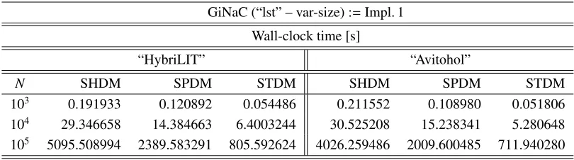
Table 3:Results from solving a SLAE on the two clusters applying the first implementation.

GiNaC (“lst” – var-size) :=Impl. 1 Wall-clock time [s]

“HybriLIT” “Avitohol”

N SHDM SPDM STDM SHDM SPDM STDM

103 _0.191933 _0.120892 _0.054486 _0.211552 _0.108980 _0.051806

104 _29.346658 _14.384663 _6.4003244 _30.525208 _15.238341 _5.280648

105 _{5095.508994 2389.583291 805.592624} _{4026.259486 2009.600485 711.940280}

Table 4:Results from solving a SLAE on the two clusters applying the second implementa-tion.

GiNaC (“matrix” – fixed-size) :=Impl. 2 Wall-clock time [s]

(4)

Table 5:Results from solving a SLAE on the two clusters applying the third implementation.

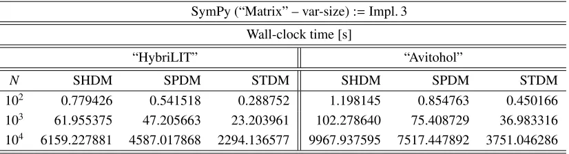
SymPy (“Matrix” – var-size) :=Impl. 3 Wall-clock time [s]

102 _0.779426 _0.541518 _0.288752 _1.198145 _0.854763 _0.450166

103 _61.955375 _47.205663 _23.203961 _102.278640 _75.408729 _36.983316

104 _{6159.227881 4587.017868 2294.136577} _{9967.937595 7517.447892 3751.046286}

Table 6:Results from solving a SLAE on the two clusters applying the fourth implementa-tion.

SymPy (“Matrix” – fixed-size) :=Impl. 4 Wall-clock time [s]

103 _0.875309 _0.726237 _0.417078 _1.272449 _0.788081 _0.429694

104 _8.420457 _5.780376 _2.909977 _12.807111 _7.738780 _4.163307

105 _{84.977702 60.360366 29.446712} _{128.940536 77.026990 41.930210}

Table 7:Results from solving a SLAE on the two clusters applying the fifth implementation.

SymPy (“MutableDenseNDimArray” – fixed-size) :=Impl. 5 Wall-clock time [s]

103 _0.730619 _0.545021 _0.308278 _1.104916 _0.694794 _0.387745

104 _7.472471 _4.941960 _3.115306 _11.105768 _6.726764 _3.759721

105 _{73.927031 51.304943 30.917188} _{111.968824 67.404472 37.466753}

Using the following formula (k– unknown coefficient of proportionality,ti– time,Ni– the matrix’s number of rows,i=1,2):

t≈kNα _⇒ t2 t1 =

_N

2 N1

α

⇔ α(N1,N2)=_log(log(_Nt2₂₎)₋−log(_log(t_N1)₁₎,

the order of growth of execution timeαfor all the five implementations was estimated (see Table 8).

(5)

Table 8:Estimation of the orderα(104_,₁₀5_).

α(104_,₁₀5₎

Impl. #1 #2 #3 #4 #5 #1 #2 #3 #4 #5 SHDM 2.24 1.00 2.00 1.00 1.00 2.12 0.98 1.99 1.00 1.00

SPDM 2.22 1.00 1.99 1.02 1.02 2.12 0.99 2.00 1.00 1.00 STDM 2.10 1.00 2.00 1.01 1.00 2.13 0.99 2.01 1.00 1.00

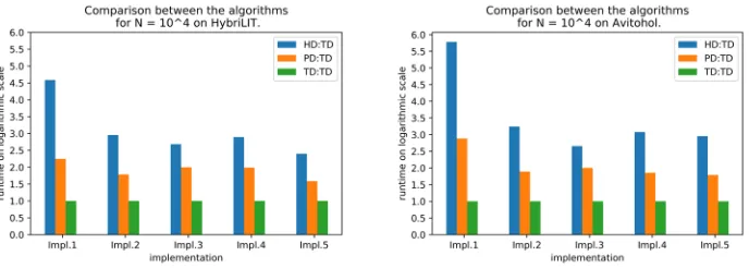
a PD SLAE to be transformed into a TD one is 23N−52, whereNis the matrix’s number of rows. This observation is relevant to Figure 1 which depicts the factors of time growth HD:TD, PD:TD, TD:TD for each of the implementations.

Figure 1:Comparison between the algorithms forN=104.

3 Discussion and Conclusions

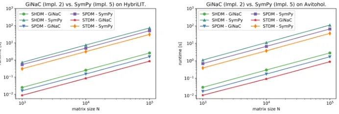
Direct comparison between the five implementations shows that the bestGiNaCone is Impl. 2, while the bestSymPyone is Impl. 5 (see Figure 2). Expectedly, theGiNaCimplementations of the three algorithms yield a much better computation time in comparison with the respected

SymPyimplementations with the difference being between one and two orders of magnitude.

It must be mentioned that the matrix class inSymPyis a subclass of the ndarray. This means that every call on a matrix object requires a few extraPythoncalls. This usually leads to a little slower performance although the difference is negligible. Figures 3 and 4 depict a

comparison of the execution time of the bestGiNaCandSymPyimplementations on the two clusters. As one can see, “HybriLIT” behaves better than “Avitohol” with the difference being

bigger when theSymPyis of interest. It is obvious that the implementations which rely on variable-size storing classes (that are Impl. 2 and Impl.3) were found to be much slower than the ones which use fixed-size storing classes, but while this was expected, it does not belittle their importance since there is a class of problems where the size of the matrix is unknown at runtime.

(6)

Figure 2:Comparison between the implementations forN=104.

Figure 3:Comparison of the execution time of the bestGiNaCandSymPyimplementations on the two clusters.

a linear complexity. This means that even if theoretically the execution time has to grow as

(7)

Figure 2:Comparison between the implementations forN=104.

a linear complexity. This means that even if theoretically the execution time has to grow as

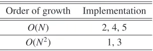
O(N), the two implementations which rely on variable-size storing classes show time growth as O(N2_{), with Impl. 1 even having} _{α >} _{2. Hence, the variable-size of the storing class} changes the order of complexity with one order of magnitude.

Table 9:Order of time growth.

Order of growth Implementation

O(N) 2, 4, 5

O(N2₎ _{1, 3}

The choice of a programming language depends on a lot of factors. However, in the con-text of symbolic computations for solving a SLAE with a band coefficient matrix (length of

band equal to 3, 5 or 7) among the options suggested in this work, we can note the following:

Pythonis easier to learn and easier and faster to prototype (no need for memory

manage-ment, build systems, compilers, etc.), on the other hand, C++has better performance and occupies less memory, but requires much more attention to bookkeeping and storage details. The authors want to express their gratitude to the Summer Student Program at JINR, Dr. Ján Buša Jr. (JINR), Dr. Andrey Lebedev (GSI/JINR), Assoc. Prof. Ivan Georgiev (IICT & IMI, BAS), the “Hy-briLIT” team at LIT, JINR, and the “Avitohol” team at the Advanced Computing and Data Centre of IICT, BAS. Computer time grants from LIT, JINR and the Advanced Computing and Data Centre at IICT, BAS are kindly acknowledged. The work is partially supported by the Russian Foundation for Basic Research under project #18-51-18005. All the figures in this paper have been generated using Matplotlib(2.1.0) [15].

References

[1] Veneva, M., Ayriyan, A.: Symbolic Algorithm for Solving SLAEs with Heptadiagonal Coefficient Matrices. Mathematical Modelling and Geometry,6, 3, 22–29 (2018).

[2] Karawia, A. A.: A New Algorithm for General Cyclic Heptadiagonal Linear Sys-tems Using Sherman-Morrisor-Woodbury Formula. ARS Combinatoria,108, 431–443 (2013).

[3] Askar, S. S., Karawia, A. A.: On Solving Pentadiagonal Linear Systems via Trans-formations. Mathematical Problems in Engineering. Hindawi Publishing Corporation. 2015, 9 (2015), doi: 10.1155/2015/232456.

[4] El-Mikkawy, M.: A Generalized Symbolic Thomas Algorithm. Applied Mathematics. 3, 4, 342–345 (2012), doi: 10.4236/am.2012.34052.

[5] Veneva, M., Ayriyan, A.: Effective Methods for Solving Band SLAEs after Parabolic

Nonlinear PDEs. AYSS-2017, European Physics Journal – Web of Conferences (EPJ-WoC).177, 07004 (2018).

[6] Veneva, M., Ayriyan, A.: Performance Analysis of Effective Methods for Solving Band

Matrix SLAEs after Parabolic Nonlinear PDEs. Advanced Computing in Industrial Mathematics, Revised Selected Papers of the 12th Annual Meeting of the Bulgarian Section of SIAM, December 20–22, 2017, Sofia, Bulgaria, Studies in Computational Intelligence,793, 407–419 (2019), doi: 10.1007/978-3-319-97277-0_33.

(8)

[8] Supercomputer System Avitohol at IICT-BAS, http://www.hpc.acad.bg/.

[9] Bauer, C., Frink, A., Kreckel, R.: Introduction to the GiNaC Framework for Symbolic Computation within the C++Programming Language. J. Symbolic Computation.33, 1–12 (2002), doi: 10.1006/jsco.2001.0494.

[10] ISO/IEC. (2012). ISO International Standard ISO/IEC for Programming Language C++. [Working draft], N3337. Geneva, Switzerland: International Organization for Standardization (ISO). Retrieved from https://isocpp.org/std/the-standard.

[11] CMake. The Cross Platform Build System. Kitware Inc. (2018), https://cmake.org. [12] Meurer, A., Smith, C. P., Paprocki, M., ˇCertík, O., Kirpichev, S. B., Rocklin, M.,

Kumar, A., Ivanov, S., Moore, J. K., Singh, S., Rathnayake, T., Vig, S., Granger, B. E., Muller, R. P., Bonazzi, F., Gupta, H., Vats, S., Johansson, F., Pedregosa, F., Curry, M. J., Terrel, A. R., Rouˇcka, Š., Saboo, A., Fernando, I., Kulal, S., Cimrman, R., Scopatz, A.: SymPy: Symbolic Computing in Python. PeerJ Computer Science.3, e103 (2017), doi: 10.7717/peerj-cs.103.

[13] Python Core Team (2015). Python: A Dynamic, Open Source Programming Language. Python Software Foundation, https://www.python.org/.

[14] Anaconda Software Distribution. Computer Software. Anaconda (2018), https://anac onda.com.