Ensemble Prediction Model with Expert Selection for
Electricity Price Forecasting
Bijay Neupane1, Wei Lee Woon2and Zeyar Aung2,*
1 Department of Computer Science, Aalborg University, Aalborg 9100, Denmark; bj21.neupane@gmail.com 2 Department of Electrical Engineering and Computer Science, Masdar Institute of Science and Technology,
Abu Dhabi, UAE; wwoon@masdar.ac.ae
* Correspondence: zaung@masdar.ac.ae; Tel.: +971-50-131-0423
Abstract:Day-ahead forecasting of electricity prices is important in deregulated electricity markets for all the stakeholders: energy wholesalers, traders, retailers, and consumers. Electricity price forecasting is an inherently difficult problem due to its special characteristic of dynamicity and non-stationarity. In this paper, we present a robust price forecasting mechanism that shows resilience towards aggregate demand response effect and provides highly accurate forecasted electricity prices to the stakeholders in a dynamic environment. We employ an ensemble prediction model in which a group of different algorithms participate in predicting the price for each hour of a day. We propose two different strategies, namely, Fixed Weight Method (FWM) and Varying Weight Method (VWM), for selecting each hour’s expert algorithm from the set of participating algorithms. In addition, we utilize a carefully engineered set of features selected from a pool of features derived from information such as past electricity price data, weather data, and calendar data. The proposed ensemble model offers better results than both the Pattern Sequence-based Forecasting (PSF) method and our own previous work using Artificial Neural Networks (ANN) alone do on the datasets for New York, Australian, and Spanish electricity markets.
Keywords:electricity price forecasting; ensemble model; expert selection
1. Introduction
Deregulated electricity markets are more and more common recently along with the evolving smart grid initiatives. In a traditional fixed-priced electricity market, consumption of electricity follows a distinct and more-or-less regular peak demand curve. This peak demand forces the supplier to use resources to meet the peak demand and those resources are redundant for rest of the time. To overcome this inefficiency, the concept of demand management is put forward as a part of the smart grid initiative [1]. A smart grid utilizes the information about the behaviors of supplier and consumers of electricity and tries to optimize the production and the distribution of electricity.
The smart grid enable a two-way peer-to-peer communication between the energy supplier (e.g., a retailer) and the consumers. This distributed information flow which takes an Internet-like form will enable the supplier to price the energy based on the consumption feedback from the consumer. On the other hand, the consumers can also schedule their consumption behavior to achieve optimal utilization at a lowest possible cost. In addition, nowadays a substantial portion of energy is generated from renewable resources like wind and solar, which are naturally less predictable than the traditional resources like fossil fuel. All these factors creates a dynamism in the electricity market, under which the main concern for the supplier is to manage a healthy ratio between demand and supply. The general idea of demand management is to design a pricing mechanism which decides the hourly prices that can persuade the consumers to change their usage patterns in order to lower the peak demand, with the expectation that the consumers will respond to it. Another objective of this mechanism is to eliminate fluctuations in the demand beyond a defined threshold.
decision on the time to buy the desired amount electricity from the market. Thus, a cost-conscious consumer will be interested about the possible electricity prices in the coming hours, days, or even weeks, and will try to optimize his/her utilization and minimize the total bill through a smart usage of electricity. With dynamic pricing systems where the consumers would pay based on their time of consumption and the amount of load they consume, it is essential for the consumers to have some price prediction mechanism to assist in scheduling their energy consumption strategy in advance.
In addition to the end consumers, price forecasting is equally important for other stakeholders in the deregulated electricity markets like the wholesalers, the traders, and the retailers. The ability to accurately forecast the future wholesale prices will allow them to perform effective planning and efficient operations, leading to ultimate financial profits for them.
The problem of electricity price forecasting is related yet distinct from that of electricity load (demand) forecasting [2–5]. Although the load and the price are correlated, their relation is non-linear. The load is influenced by various factors such as non-storability of electricity, consumers’ behavioral patterns, and seasonal changes in demand. The price, on the other hand, is affected by those aforesaid factors as well as additional aspects such as financial regulations, competitors’ pricing, dynamic market factors, and various other macro- and micro-economic conditions. As a result, the price of electricity is a lot more volatile than the electricity load. Interestingly, when dynamic pricing strategies are introduced, prices become even more volatile, where the daily average price changes by up to 50% while other commodities generally exhibit only about 5% of change in maximum [6]. A number of research works have been performed on electricity price forecasting [7–10]. However, to our best knowledge, none of them is able to provide adequately accurate results consistently for all the cases for the respective experimental data of their target market. Thus, a more accurate price forecasting system is necessary to facilitate all the stakeholders, where the consumers’ consumption patterns will depend on the future electricity prices, and so are the businesses of the wholesalers, the traders, and the retailers.
A good price forecasting system should consider different factors associated with dynamic pricing scheme in the smart grid and should be able to tackle it in an efficient manner. One of the main challenges in price forecasting under a dynamic pricing scheme is to overcome the aggregate demand response effect from the consumers which causes sharp rises in peak demand triggering sharp changes in prices. Different consumers have different priorities regarding the utilization of electricity under a dynamic pricing scheme, thus their responses to a certain price value might vary substantially. This unpredictable behavior of the consumer might causes high fluctuations in the demand curve which in turn causes higher fluctuations in electricity prices in a circular manner.
In order to address the above challenges in electricity price forecasting, in this paper, we propose an ensemble learning model with the following characteristics:
• We use a carefully engineered set of features taken from the pool of features derived from information such as past electricity price data (from multiple view points), weather data, and calendar data.
• For each participating learning algorithm, we use a wrapper method for feature selection in which the algorithm is continuously trained and updated in order to select the best feature set. • We propose two different ensemble models, namely Fixed Weight Method (FWM) and Varying
Weight Method (VWM). The final prediction is tentatively based on the assigned weight of the selected learning algorithm (denoted as an “expert”).
• In order to tackle the fluctuation and aggregate demand response effect, we introduce a fallback mechanism to ensure that the prediction accuracy lies within a desirable range.
been proposed in different fields, e.g., crude oil price [16] and carbon price [17]. However, to our best knowledge, our proposed model is the first to utilize ensemble learning involving different participating algorithms for the purpose of electricity price forecasting.
2. Related Work
Electricity price forecasting has become one of the most significant aspects in deregulated electricity markets for planning, production, and trading. The positive economic consequences have attracted many stakeholders to invest time and money for development of new methods for precise price prediction. This financial aspect has drawn immense interest to many researchers, and has produced many significant research and contribution in electricity price forecasting. This research thrust gains more momentum with the introduction of smart grid. The papers [7–10] provide good surveys on various methods of electricity price forecasting. We will discuss some of the existing electricity price forecasting methods below.
In [18], the authors proposed an Autoregressive Integrated Moving Average (ARIMA)-based statistical model of electricity price forecasting. The model was based on wavelet transformation where final forecasted results were obtained by applying inverse wavelet transformation. In [6], the proposed method was an augmented ARIMA model which was an enhancement of Box and Jenkins [19] model. Tan et al. [20] performed electricity price forecasting using wavelet transform combined with ARIMA and another statistical model, namely Generalized Autoregressive Conditional heteroskedasticity (GARCH). The work in [21] applied a mixture of wavelet transform, linear ARIMA, and nonlinear neural network models to predict normal prices and price spikes separately.
In [22–24], the authors proposed different prediction models using artificial neural network (ANN). Each proposed model utilized different set of features created using historical market clearing price, system load, and fuel price. The range of model varies from a simple three-layer architecture to combination models including Probability Neural Network (PNN) and Orthogonal Experimental Design (OED). In [24], the author implemented PNN as a classifier which showed advantage of a fast learning process as it requires a single-pass network training stage for adjusting weights. OED was used to find the optimal smoothing parameter which help to increase prediction accuracy.
In [25,26], the authors proposed price prediction models using Support Vector Regression (SVR). The work in [25] used projected Assessment of System Adequacy (PASA) data as one of the inputs for the model and that in [26] implemented Artificial Fish Swarm Algorithm (AFSA) for choosing the parameter of SVM models.
Other diverse approaches for electricity price forecasting include Self-Organizing Map (SOM) [27], hybrid Principal Component Analysis (PCA) [28], Fuzzy Inference [29], Particle Swarm Optimization (PSO) [30], etc.
In [11], Martínez-Álvarez et. al presented a method which was based on pattern sequence similarity. In this approach, a clustering technique was first used on the data before application of the Pattern Sequence-based Forecasting (PSF) algorithm to produce one step ahead forecasts of the electricity prices. In the experiment, k-means clustering was used to cluster the training data. The training is performed using data collected from 3 different electricity markets, namely New York (NYISO) [13], Australia (ANEM) [14], and Spain (OMEL) [15], for the years 2004–2005, while testing is carried out for using data from 2006. The authors perform a detailed analysis using these three different datasets, and compared their results to those obtained using other methods. As this work is relatively recent and the three datasets used are publicly available, we use the results described in this research as benchmarks in order to evaluate those obtained by our proposed ensemble-based method.
2008–2012 datasets from the same markets. The ANN-based model showed promising results and was able to obtain higher forecasting accuracy compared to PSF. The results of our newly proposed ensemble-based model are also compared with those obtained from this ANN-only approach.
3. Proposed Prediction Model
Our objective is to develop a robust model which can sustain its good performance irrespective of various uncertainty factors. For that, we propose an ensemble prediction model which provides flexibility in choosing the type of algorithm for price prediction. This flexibility enables the user to choose the algorithm based on available resources, time constraints, and computational complexity.
We believe that incorporating the modified ensemble learning [31] scenario into the well-known prediction methods will help to improve the performance of the prediction model. With the current research on price prediction, machine learning algorithms like Artificial Neural Network (ANN) [32], Support Vector Regression (SVR) [33], and Random Forest (RF) [34] showed promising results. We propose an ensemble learning strategy which enables these algorithms to learn from the environment and update their parameters based on the information they have collected.
3.1. Model Formulation
Consider a wholesale electricity market where a retailer proposes a bidding price based on the present information he has (i.e., the predicted price). Once the actual price is known, the retailer can evaluate authoritativeness of the provided information. He wants to minimize the difference of the actual market price and the predicted price information provided to him by the forecasting algorithm. Now, let us consider an ensemble forecasting model involving a number of forecasting algorithms. Let A = {a1,a2,a3, . . . ,an}denote a set of participating forecasting algorithms, where
nis the number of participating algorithms andai(1≤i≤n)is an individual participating algorithm. The should be noted that we treat each individual hour of the day separately. Thus, in total, we build 24 separate ensemble forecasting models — one for each hourh ∈ {1, . . . , 24}of the day. For the sake of simplicity, we omit this hour parameter in our description of the proposed model below. So, unless stated otherwise, all the variables used below belong to an individual hourhof the day.
We defineprediction errormade by an algorithmx, wherex∈Aas follows:
prediction error: Ex=|P
0
x−P| (1)
wherePis the actual electricity price, andPx0 is the predicted price by the algorithmx.
Let us defineWi (1≤i≤n) as the past performance “weight”of the algorithm ai. (Later we will discuss how we compute the performance weight using the two algorithms, Fixed Weight Method (FWM) or Varying Weight Method (VWM), respectively.)
Among all the algorithms a1,a2,a3, . . . ,an, we select the algorithm whose past performance weightWiis the highest as today’s“expert” algorithm. We denote the expert algorithm as ˆa.
expert algorithm:aˆ=arg max ai∈A
(Wi) (2)
Suppose we make the observations of our forecasting process formnumber of days. Then, we have a list ˆAof containingmexpert algorithms.
list of experts: Aˆ = [aˆ1, ˆa2, . . . , ˆam] (3) Our expectation is that overmdays, the overall performance of the list ˆA’s expert algorithms on their corresponding days should be superior to that of any individual participating algorithm acting alone. In order words, the cumulative prediction error incurred by our selected expert algorithms should be less than that of any individual algorithm. Formally, we should have:
m
∑
j=1
Eaˆj ≤ m
∑
j=1
Exj, ∀x∈A (4)
So, in our proposed algorithms, as a fallback mechanism, we regularly check the above constraint in Equation 4. Once we find that the past Cumulative prediction error of the selected expert algorithms overmdays is worse than that of any of the individual algorithms, we take the forecasting output by the best individual algorithm as the final prediction result – instead of the taking the forecasting output of the selected expert algorithm. In addition, we update all the individual participating algorithms by re-training them with all the available data to date. This strategy enables us to tackle the effect of concept drift [35], which usually occurs in time-series data like electricity prices.
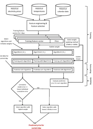
3.2. Model Architecture
Our model proposed for electricity price prediction is presented in Figure1. We have to recruit prediction algorithms which exhibits promising result when utilized separately to participate in our ensemble model. Here we show three participating algorithms for demonstration purpose. (In theory, any number of different algorithms can be used under this model depending upon the processing power and time available.) The proposed model performs feature engineering on the price data along with the corresponding temperature and calendar data collected from a de-regulated electricity market, which is followed by feature selection, learning, predicting, and model updating steps.
Prediction is made by the all the participating algorithms, but the decision will be made only by the algorithm whose performance was best recently in the previous days. On the first day of the model deployment, the expert algorithm will be chosen randomly. From the second day onward, for each hour of the day, the performance of each algorithm will be evaluated and the best algorithm will be chosen based on their past prediction accuracy. The best predictor will be the expert predictor, whose predicted value for next day will be the decisive value. At the end of each day when the actual price becomes available, every algorithm will analyze their performance for that day. If the performance is within the range of the threshold, the models are maintained. Otherwise, the models are updated by re-training them with all the available data up to date. The proposed ensemble models, using fixed weights and varying weights respectively, are described in Algorithms 1 and 2.
It should be noted that both algorithms for designed for each individual hour of the day. So, for each algorithm, we need to run 24 separate instances of it to forecast the electricity prices for 24 hours.
3.2.1. Algorithm 1: Fixed Weight Method (FWM)
Figure 1. Overview of the proposed ensemble model demonstrated with three participating algorithms.
Algorithm 1Fixed Weight Method (TrainSet[1 ..t],TestSet[1 ..m]) 1: choose the setAofnparticipating algorithms:A={a1,a2,a3, . . . ,an}
2: Aˆ←[ ]; /* initialize list of experts */
3: e←random(1 ..n);We←1; /* randomly select an algorithm as expert and assign its weight as 1 */
4: fori←1 tondo 5: ifi6=ethen
6: Wi←0; /* initialize weights of all algorithms except expert’s as 0 */
7: end if
8: mj←Train(ai,TrainSet[1 ..t]); /* build prediction modelmiby training algorithmaiusing data in the training set for days 1 ..t*/
9: CumuError[i]←0; /* initialize cumulative prediction error of all algorithms as 0 */
10:end for
11:ExpertCumuError←0; /* initialize cumulative prediction error of list of experts as 0 */
12:retrain←FALSE;
13:
14:forj←1 tomdo
15: /* for allmnumber of days inTestSet, do the following three steps */
16:
17: /* step 1: carrying out prediction */
18: fori←1 tondo
19: /* apply prediction modelmiof algorithmaiusing data in the training set plus those in the testing set up until previous day */
20: Pai0 ←GetPrediction(mi,ai,TrainSet∪TestSet[1 ..j−1]);
21: ifWi=1then
22: aˆ←ai; /* if weight is 1, then it is the current expert */
23: add ˆato list ˆA; /* insert the current expert into list of experts */
24: PredictedPrice←Pa0ˆ; /* tentatively, predicted price will be output of the current expert */
25: end if
26: end for
27:
28: /* step 2: fallback procedure and reporting */
29: l←arg mini=1..nCumuError[i]; /*lis index of algorithm with lowest cumulative error */
30: ifCumuError[l]<ExpertCumuErrorthen
31: PredictedPrice←Pal0; /* take algorithml’s output instead of expert algorithm’s */
32: retrain←TRUE; /* all models must be updated later */
33: end if
34: reportPredictedPrice; /* report predicted price forjthday as our output */ 35:
36: /* step 3: prediction error calculation and updating — after actual pricePof dayjis known */
37: Eˆa←P
0
ˆ
a−P; /* calculate expert algorithm’s prediction error */
38: ExpertCumuError←ExpertCumuError+Eˆa;
39: fori←1 tondo
40: Eai←Pai0 −P; /* calculate all algorithms’ prediction errors */
41: CumuError[i]←CumuError[i] +Eai;
42: end for
43: We←0; /* reset weight of old expert to 0 */
44: e←arg mini=1..nP
0
ai; /* select algorithm with lowest error forjthday as new expert for(j+1)thday */
45: We←1; /* set weight of new expert as 1 */
46: /* re-train models if required */
47: ifretrain=TRUEthen
48: fori←1 tondo
49: mi←Train(ai,TrainSet∪TestSet[1 ..j]); /*update all models using the latest available data till now */
50: end for
51: retrain=FALSE; /* resetretrainflag */
52: end if
53:end for
3.2.2. Algorithm 2: Varying Weight Method (VWM)
its weight increased and other algorithm with lower accuracy will have their weight decreased based on prediction accuracy achieved by them. The main benefit of this model is that it considers the individual prediction error value when updating the weight. So the weight of any algorithm is dependent on the cumulative error and number of times it has been the best predictor.
Algorithm 2Varying Weight Method (TrainSet[1 ..t],TestSet[1 ..m],λ) 1: choose the setAofnparticipating algorithms:A={a1,a2,a3, . . . ,an}
2: Aˆ←[ ]; /* initialize list of experts */
3: e←random(1 ..n); /* randomly select an algorithm as expert */
4: fori←1 tondo
5: Wi←1; /* initialize weights of all algorithms as 1 */
6: mj←Train(ai,TrainSet[1 ..t]); /* build prediction modelmiby training algorithmaiusing data in the training set for days 1 ..t*/
7: CumuError[i]←0; /* initialize cumulative prediction error of all algorithms as 0 */
8: end for
9: ExpertCumuError←0; /* initialize cumulative prediction error of list of experts as 0 */
10:retrain←FALSE;
11:
12:forj←1 tomdo
13: /* for allmnumber of days inTestSet, do the following three steps */
14:
15: /* step 1: carrying out prediction */
16: fori←1 tondo
17: /* apply prediction modelmiof algorithmaiusing data in the training set plus those in the testing set up until previous day */
18: Pai0 ←GetPrediction(mi,ai,TrainSet∪TestSet[1 ..j−1]);
19: end for
20: ifj6=1then
21: e←arg maxi=1..nWi /* if weight is the highest, then it is the current expert */
22: end if
23: aˆ←ae; add ˆato list ˆA; /* insert the current expert into list of experts */
24:
25: PredictedPrice←Pa0ˆ; /* tentatively, predicted price will be output of the current expert */
26:
27: /* step 2: fallback procedure and reporting */
28: l←arg mini=1..nCumuError[i]; /*lis index of algorithm with lowest cumulative error */
29: ifCumuError[l]<ExpertCumuErrorthen
30: PredictedPrice←Pal0; /* take algorithml’s output instead of expert algorithm’s */
31: retrain←TRUE; /* all models must be updated later */
32: end if
33: reportPredictedPrice; /* report predicted price forjthday as our output */ 34:
35: /* step 3: prediction error calculation and updating — after actual pricePof dayjis known */
36: Eˆa←P
0
ˆ
a−P; /* calculate expert algorithm’s prediction error */
37: ExpertCumuError←ExpertCumuError+Eˆa;
38: fori←1 tondo
39: Eai←Pai0 −P; /* calculate all algorithms’ prediction errors */
40: CumuError[i]←CumuError[i] +Eai;
41: end for
42: s←arg mini=1..nEai /*sis index of algorithm with smallest prediction error for current dayj*/
43: /* update weights */
44: fori←1 tondo 45: ifi=sthen
46: Wi←Wi×(Eai×λ) /* increase weight of algorithmaiby factor ofλandEai*/
47: else
48: Wi←Wi/(Eai×λ) /* decrease weight of algorithmaiby factor ofλandEai*/
49: end if
50: end for
51: /* re-train models if required */
52: ifretrain=TRUEthen
53: fori←1 tondo
54: mi←Train(ai,TrainSet∪TestSet[1 ..j]); /*update all models using the latest available data till now */
55: end for
56: retrain=FALSE; /* resetretrainflag */
57: end if
58:end for
3.3. Data Preprocessing
3.3.1. Feature Engineering
The electricity market data follows a time series pattern and provides the information about the daily electricity prices over a period of time. The information its raw form does not contain any specific features (attributes) that can be used in electricity price prediction. So, from the time series data, we need to generate relevant features to be used in prediction models as an input. Previous researches have shown that prediction models are often affected by higher variance in time series data. Thus, feature generation a.k.a. feature engineering is one of the important aspects in building the prediction model, where the features are carefully created to reduce over-fitting of the model and accurately capture the target value. In our previous work, [12] we have shown that generating relevance features from single or a few sources improves the predictions accuracy of the model by a significant margin. In this research, we have engineered 47 different features to capture various hidden trends in the electricity market.
In order to predict the hourh’s electricity price, we extract the hourly price data for the past 24 hours (h−1 toh−24) window yielding 24 different features. The features which can best represent the short term trend in electricity market are the previous 24 hours data, as observed in [36]. This data provides us a good insight for short term trends but fails to capture seasonal and long term trends. To order to build a robust prediction model, both short and long terms and seasonal effect should be captured efficiently. Sudden high fluctuation in electricity price might occur due to the seasonal behavior and other factors. In order to capture these uncertain behaviors in electricity price, we created putatively relevant features based on historical time series electricity price dataset. So, 20 additional features like last year same day same hour price, last year same day same hour price fluctuation, last week same day same hour price, last week same day price fluctuation etc. were created.
In order to achieve an even better forecasting accuracy, we also introduce various features which are not directly associated with price data. We explore various other factors that can affect the electricity load and the price of the market. We have found that according to [8], the temperature, the day of the week, and the occurrence of holidays can all affect the electricity load and price. Therefore, we also incorporate these 3 non-price features into our generated feature set. For the temperature features, we use historical and forecasted temperature data provided by Weather Underground [37]. For the holiday data, we use predefined holiday information in the geographical area of the target electricity market.
It should be noted that oil and gas prices and other factors like load and types of resources used for electricity generation might also affect the pricing. However, for the three target markets in out studies (namely, New York, Australia, and Spain), these data are not easily accessible to us, and we leave them to be considered in our future work.
Normalization is one of the best approach to deal with the input data where the attributes are of different measurements and scales. In our case, as we use various input data with different scales, we need to normalize all the 47 attributes to achieve consistency. We use the mapminmaxfunction available in Matlab [38] to normalize our input data. This function returns a normalized matrix by normalizing each row to the range of provided minimum and maximum values. We normalize all the attributes into the range(−1.0, 1.0).
3.3.2. Feature Selection
Though 47 features were created using the historical electricity price, calendar, and weather data, using all the created features for building model poses the threat of over-fitting. All the generated features are analyzed to remove redundant, irrelevance, and loosely coupled features. Thus, feature selection process is used to select the most relevance features from the original feature set.
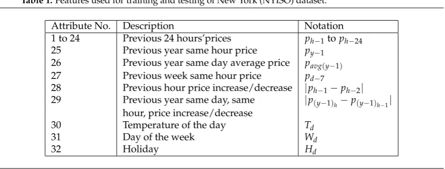
Table 1.Features used for training and testing of New York (NYISO) dataset.
Attribute No. Description Notation
1 to 24 Previous 24 hours’prices ph−1toph−24
25 Previous year same hour price py−1
26 Previous year same day average price pavg(y−1)
27 Previous week same hour price pd−7
28 Previous hour price increase/decrease |ph−1−ph−2|
29 Previous year same day, same |p(y−1)h−p(y−1)h−1| hour, price increase/decrease
30 Temperature of the day Td
31 Day of the week Wd
32 Holiday Hd
and evaluate the subset using the model or learning algorithm. Wrapper evaluates the estimated accuracy obtained from learning algorithm by adding or removing features from the features subset. Estimation of accuracy is done using cross validation, in this research we have implemented 10 fold cross validation on the training set and Artificial Neural Network (ANN) is used as the learning algorithm. Wrappers methods are most widely used in supervised learning problem where labels are available.
In selecting the best feature set, the wrapper method is applied to all features except those associated with the past 24 hours. Technically, this training accuracy may be less than the best possible accuracy since we did not incorporate the past 24 hour data. Once we apply all the data, including the past 24 hour data, to the wrapper, it take a much longer time since the wrapper method is computationally very expensive. Due to the verified importance of the past 24 hour data [36], we choose to exclude it from our feature selection using the wrapper and select the best features from the remaining ones (23 of them) with the wrapper using 10 fold cross validation.
The final feature set obtained for New York (NYISO) dataset after feature selection process is shown as an example in Figure1.
4. Experimental Setup
4.1. Data
We evaluated our proposed ensemble model by performing experiment with dataset from three different deregulated electricity markets of New York (NYISO) [13], Australia (ANEM) [14], and Spain (OMEL) [15]. We selected data from these markets to compare the results of our proposed model with those in the previous works. As mentioned in [11], a vast amount of research has been carried out using the data from these markets. NYISO electricity market contains data from various areas from New York and provides data for hourly electricity price. From NYISO, we selected “Capita”˙Ias the reference area to benchmark our results with those of the previous works [11,12]. ANEM represents the market clearing data in Australian market since its deregulation with half hour resolution. Again, we selected the data from “Queensland” area to be consistent with the experiments in those two previous works. Likewise, for the Spanish (OMAL) market, we also used the same data as those previous works.
4.2. Evaluation Metrics
Mean Error Relative to P (MER)
MER=100× 1
N
N
∑
i=1
|Pi−P
0
i| ¯
P (5)
wherePidefines the actual price andP
0
i defines the predicted price. ¯Pis the mean price for the period of interest and N is the number of predicted hours. This indicator is irrespective of the absolute values.
Mean Absolute Error (MAE)
MAE= 1 N
N
∑
i=1
|Pi−P
0
i| (6)
The indicator is dependant on the absolute range of the electricity price.
Mean Absolute Percentage Error (MAPE)
MAPE=100× 1
N
N
∑
i=1
|Pi−P
0
i|
Pi
(7)
This indicator is irrespective of the absolute values. If the range of the electricity price is vast, a prediction may give a high MAE value, but a low MAPE.
5. Experimental Results
Two different sets of experiments (Experiments I and II) were performed using two different time periods, 2004–2006 (on NYISO, ANEM, and OMEL datasets) and 2008–2012 (on NYISO and ANEM datasets) respectively.
5.1. Experiment I: 2004–2006
In Experiment I, the NYISO, ANEM, and OMEL datasets for the time period of 2004–2006 are used. For all the datasets, we use the data of March 2004–March 2006 as the training set and April 2006–December 2006 as the testing set. We use the exact same experimental protocol as in Martínez-Álvarezet. al[11]. The following four methods are compared.
1. Ensemble learning using Fixed Weight Method (FWM) (Algorithm1) using three participating machine learning algorithms: Artificial Neural Network (ANN), Support Vector Regression (SVR), and Random Forest (RF),
2. Ensemble learning using Varying Weight Method (VWM) (Algorithm 2) using the same participating algorithms as in FWM,
3. Artificial Neural Network only (ANN-only) (as presented in our previous work [12]), and 4. Pattern Sequence-based Forecasting (PSF) (by Martínez-Álvarezet. al[11]).
5.1.1. Experiment I-A: NYISO Dataset
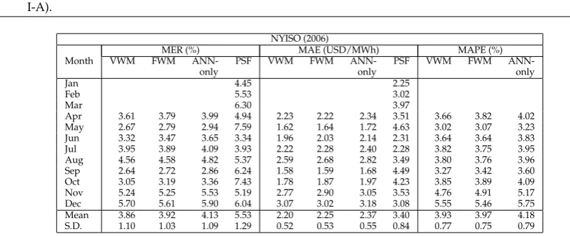
Table2shows mean error rate (MER) (Equation5), mean absolute error (MAE) (Equation5), and mean absolute percentage error (MAPE) (Equation7) of the four methods for New York (NYISO) data for the testing period of the year 2006. We can see that the results obtained from FWM (VWM in the brackets) have the average MER of 3.92% (3.86%) with the S.D. (standard deviation) of 1.03 (1.10), MAE of USD2.25/MWh (USD2.20/MWh) with S.D. of 0.53 (0.52), and MAPE of 3.97% (3.93%) with S.D. of 0.75 (0.77). The worst month is December 2006 where MER is 5.61% (5.70%), MAE is 3.02 (3.07) and MAPE is 5.46% (5.55%).
VWM offers slightly better results than FWM with the improvements (decreases in error) of 0.06% of MER, USD0.05/MWh of MAE, and 0.04% of MAPE.
Table 2.MER, MAE, and MAPE performance indicators for NYISO market for year 2006 (Experiment I-A).
NYISO (2006)
MER (%) MAE (USD/MWh) MAPE (%)
Month VWM FWM ANN- PSF VWM FWM ANN- PSF VWM FWM
ANN-only only only
Jan 4.45 2.25
Feb 5.53 3.02
Mar 6.30 3.97
Apr 3.61 3.79 3.99 4.94 2.23 2.22 2.34 3.51 3.66 3.82 4.02 May 2.67 2.79 2.94 7.59 1.62 1.64 1.72 4.63 3.02 3.07 3.23 Jun 3.32 3.47 3.65 3.34 1.96 2.03 2.14 2.31 3.64 3.64 3.83 Jul 3.95 3.89 4.09 3.93 2.22 2.28 2.40 2.28 3.82 3.75 3.95 Aug 4.56 4.58 4.82 5.37 2.59 2.68 2.82 3.49 3.80 3.76 3.96 Sep 2.64 2.72 2.86 6.24 1.58 1.59 1.68 4.49 3.27 3.42 3.60 Oct 3.05 3.19 3.36 7.43 1.78 1.87 1.97 4.23 3.85 3.89 4.09 Nov 5.24 5.25 5.53 5.19 2.77 2.90 3.05 3.53 4.76 4.91 5.17 Dec 5.70 5.61 5.90 6.04 3.07 3.02 3.18 3.08 5.55 5.46 5.75 Mean 3.86 3.92 4.13 5.53 2.20 2.25 2.37 3.40 3.93 3.97 4.18 S.D. 1.10 1.03 1.09 1.29 0.52 0.53 0.55 0.84 0.77 0.75 0.79
Notes:
(1) For the NYISO dataset, The results for the period January–March 2006 cannot be presented for VWM, FWM, and ANN-only because
the feature vectors of their corresponding training data during the period of January–March 2005 cannot be constructed. Construction of
those training feature vectors in turn requires the data before March 2004, which is not readily available to us. For PSF, such a feature vector
construction is not required and neither are the data before March 2004.
(2) MAPE results for PSF are not presented because it was not used as an evaluation criterion in [11].
(3) The standard deviation (S.D.) results provided here are computed usingstdev(estimated standard deviation based on a sample) function in
Microsoft Excel. They are different from the ones reported in [11] and [12] which are computed by a different standard deviation function.
5.1.2. Experiment I-B: ANEM Dataset
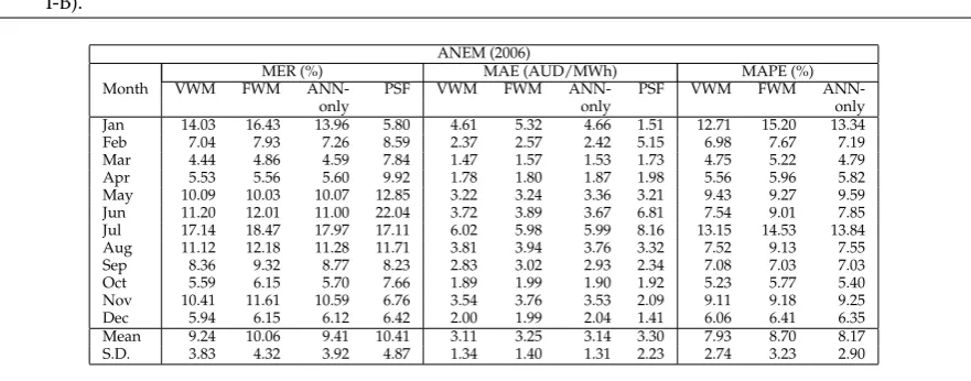
The Australian (ANEM) dataset a challenging one. It is highly volatile with a large number of unexpected abnormalities and outliers. ANEM dataset exhibits high fluctuations in electricity prices with the highest price of AUD9739/MWh in January 2006 and the lowest value of AUD7.81/MWh in February 2004. The variance and skewness for each market data will be discussed in following Section6.
Due to this highly fluctuating values and outliers, forecasted price for this market has high range of error. From Table3, we can see that performance FWM (VWM in the brackets) of on ANEM data is 10.06% (9.24%) of average MER with S.D. of 4.32 (3.83), AUD3.25/MWh (AUD3.11/MWh) MAE with S.D. of 1.40 (1.34), and 8.70% (7.93%) MAPE with S.D. of 3.23 (2.74).
Bad performances are observed for the months of January, June, July, and August 2006. The worst performance of 18.47% (17.14%) MER and 14.53% (13.15%) MAPE are obtained July 2006. The best performance of 4.86% (4.44%) MER and 5.22% (4.75%) MAPE are resulted in the month of March 2006.
Table 3.MER, MAE, and MAPE performance indicators for ANEM market for year 2006 (Experiment I-B).
ANEM (2006)
MER (%) MAE (AUD/MWh) MAPE (%)
Month VWM FWM ANN- PSF VWM FWM ANN- PSF VWM FWM
ANN-only only only
Jan 14.03 16.43 13.96 5.80 4.61 5.32 4.66 1.51 12.71 15.20 13.34 Feb 7.04 7.93 7.26 8.59 2.37 2.57 2.42 5.15 6.98 7.67 7.19 Mar 4.44 4.86 4.59 7.84 1.47 1.57 1.53 1.73 4.75 5.22 4.79 Apr 5.53 5.56 5.60 9.92 1.78 1.80 1.87 1.98 5.56 5.96 5.82 May 10.09 10.03 10.07 12.85 3.22 3.24 3.36 3.21 9.43 9.27 9.59 Jun 11.20 12.01 11.00 22.04 3.72 3.89 3.67 6.81 7.54 9.01 7.85 Jul 17.14 18.47 17.97 17.11 6.02 5.98 5.99 8.16 13.15 14.53 13.84 Aug 11.12 12.18 11.28 11.71 3.81 3.94 3.76 3.32 7.52 9.13 7.55 Sep 8.36 9.32 8.77 8.23 2.83 3.02 2.93 2.34 7.08 7.03 7.03 Oct 5.59 6.15 5.70 7.66 1.89 1.99 1.90 1.92 5.23 5.77 5.40 Nov 10.41 11.61 10.59 6.76 3.54 3.76 3.53 2.09 9.11 9.18 9.25 Dec 5.94 6.15 6.12 6.42 2.00 1.99 2.04 1.41 6.06 6.41 6.35 Mean 9.24 10.06 9.41 10.41 3.11 3.25 3.14 3.30 7.93 8.70 8.17 S.D. 3.83 4.32 3.92 4.87 1.34 1.40 1.31 2.23 2.74 3.23 2.90
5.1.3. Experiment I-C: OMEL Dataset
The results obtained from the Spanish market are shown in Table4. We can see that the average MER of FWM (VWM in the brackets) is 5.34% (5.26%) with S.D. of 0.54 (0.62), which indicates that the monthly errors are not much different from the average error. MAE for the Spanish data is EURc0.34/kWh (EURc0.35/kWh) with the S.D. of 0.03 (0.05) and MAPE of 5.75% (5.62%) with S.D. of 1.25 (1.07). MAE for OMEL dataset is very low compared to other markets because of the prices are in a different unit of measurement, which is EUR cent per kWh instead of USD/AUD per MWh in NYISO/ANEM datasets.
It can also be observed that, unlike the previous two cases of NYISO and ANEM, VWM is not always better than FWM for all three evaluation criteria. Whilst VWM is slightly better than FWM in terms of the average MER and MAPE, it is slightly worse than FWM in terms of MAE.
Table 4.MER, MAE, and MAPE performance indicators for OMEL market for year 2006 (Experiment I-C).
OMEL (2006)
MER (%) MAE (EURc/kWh) MAPE (%)
Month VWM FWM ANN- PSF VWM FWM ANN- PSF VWM FWM
ANN-only only only
Jan 5.91 5.65 6.00 7.26 0.40 0.36 0.40 0.53 5.00 4.56 5.07 Feb 5.20 5.34 5.25 4.93 0.34 0.35 0.35 0.36 3.49 3.88 3.66 Mar 5.05 5.48 5.28 5.88 0.34 0.35 0.35 0.43 6.28 6.33 6.19 Apr 5.68 6.11 5.90 3.62 0.39 0.39 0.39 0.28 5.55 5.88 5.73 May 5.88 5.60 6.00 8.11 0.40 0.36 0.40 0.64 5.88 5.69 6.11 Jun 5.12 5.36 5.14 3.76 0.33 0.35 0.34 0.29 5.05 5.68 5.27 Jul 4.68 4.59 4.59 4.30 0.29 0.30 0.30 0.33 4.59 4.52 4.55 Aug 5.10 5.07 5.17 5.37 0.33 0.33 0.34 0.42 5.50 5.39 5.57 Sep 5.61 5.44 5.66 6.41 0.36 0.35 0.37 0.50 5.36 5.03 5.42 Oct 6.04 5.78 6.08 7.89 0.41 0.37 0.40 0.58 6.31 6.23 6.64 Nov 3.83 4.10 3.94 8.30 0.25 0.27 0.26 0.64 7.13 7.91 7.25 Dec 5.06 5.50 5.04 8.02 0.33 0.36 0.33 0.59 7.33 7.94 7.61 Mean 5.26 5.34 5.34 6.15 0.35 0.34 0.35 0.47 5.62 5.75 5.76 S.D. 0.62 0.54 0.64 1.76 0.05 0.03 0.04 0.13 1.07 1.25 1.11
5.2. Experiment II: 2008–2012
RF participating algorithms), VWM (with the same participating algorithms), and ANN-only are compared. It is observed that the results our proposed model for this Experiment II are even slightly better than those in Experiment I.
5.2.1. Experiment II-A: NYISO Dataset
From Table 5, we can see that the overall performances of both FWM and VWM for this 2008–2012 NYISO dataset are even slightly better than those for the Experiment I-A (NYISO’s 2004–2006 dataset) despite the fact that the 2008–2012 data contain many spikes and outliers. For this dataset, FWM (VWM in the brackets) provides average MER of 3.86% (3.85%) with S.D. of 0.57 (0.57), MAE of USD1.48/MWh (USD1.48/MWh) with S.D. 0.54 (0.54), and MAPE 3.99% (3.94%) with S.D. of 1.45 (1.42). Noticeable improvement can be observed in MAE with a decrease of USD0.77/MWh (USD0.72/MWh) when compared to Experiment I-A.
The worst forecasting results obtained were 4.87% (4.82%) of MER in January 2012, USD2.68/MWh (USD2.71/MWh) of MAE and 7.25% (7.12%) of MAPE both in July 2011. The main reason for higher forecasting error in July 2011 and January was due to the higher numbers of spikes and outliers in those months in the New York market.
Table 5. MER, MAE, and MAPE performance indicators for NYISO market for years 2011–2012 (Experiment II-A).
NYISO (2011–2012)
MER (%) MAE (USD/MWh) MAPE (%) Month VWM FWM ANN- VWM FWM ANN- VWM FWM
ANN-only only only
Jun 4.25 4.24 4.27 1.92 1.97 2.01 5.19 5.32 4.31 Jul 4.40 4.36 4.66 2.71 2.68 2.97 7.12 7.25 4.72 Aug 3.39 3.34 3.54 1.50 1.48 1.56 3.87 3.99 3.51 Sep 3.56 3.61 3.86 1.38 1.38 1.47 3.72 3.73 3.76 Oct 3.49 3.50 3.55 1.33 1.32 1.33 3.60 3.56 3.48 Nov 3.57 3.56 3.61 1.31 1.28 1.3 3.41 3.47 3.62 Dec 3.73 3.80 4.01 1.35 1.36 1.44 3.68 3.68 4.16 Jan 4.82 4.87 4.92 2.19 2.15 2.32 5.71 5.82 5.14 Feb 3.22 3.25 3.7 1.06 1.05 1.2 2.84 2.83 3.81 Mar 4.74 4.76 4.83 1.27 1.29 1.31 3.48 3.48 4.86 Apr 3.84 3.80 4.18 0.96 0.95 1.06 2.44 2.56 4.09 May 3.22 3.23 3.45 0.84 0.83 0.88 2.18 2.25 3.27 Mean 3.85 3.86 4.05 1.48 1.48 1.57 3.94 3.99 4.06 S.D. 0.56 0.57 0.52 0.54 0.54 0.59 1.42 1.45 0.60
5.2.2. Experiment II-B: ANEM Dataset
The performances of FWM and VWM in this period for ANEM dataset are noticeably better for those of the Experiment I-B (ANEM’s 2004–2006 dataset). For this dataset, FWM (VWM in the brackets) provides average MER of 7.16% (6.98%) with S.D. of 3.83 (3.98), MAE of AUD2.09/MWh (AUD2.05/MWh) with S.D. 1.37 (1.36), and MAPE of 6.22% (6.16%) with S.D. of 3.01 (2.98). The improvements (deceases in error) over ANEM’s 2004–2006 dataset by FWM (VWM in the brackets) are 2.90% (2.26%) in MER, AUD1.16/MWh (AUD1.06/MWh) in MAE, and 2.48% (1.77%) in MAPE.
There are also decreases in S.D. for both FWM and VWM which indicate that the errors in the years 2011–2012 are less more deviated from the mean error when compared to those for the years 2004–206 in ANEM dataset.
Table 6. MER, MAE, and MAPE performance indicators for ANEM market for years 2011–2012 (Experiment II-B).
ANEM (2011–2012)
MER (%) MAE (AUD/MWh) MAPE (%) Month VWM FWM ANN- VWM FWM ANN- VWM FWM
ANN-only only only
Jun 4.11 4.32 4.6 1.15 1.20 1.28 4.42 4.34 4.62 Jul 6.85 7.01 7.46 1.98 1.95 2.07 6.59 6.52 6.94 Aug 4.73 4.76 5.06 1.30 1.32 1.41 4.07 4.18 4.44 Sep 4.05 4.17 4.43 1.13 1.16 1.23 4.02 3.99 4.25 Oct 4.19 4.36 4.64 1.15 1.21 1.29 4.08 4.29 4.57 Nov 6.90 6.89 7.33 1.88 1.91 2.03 5.52 5.73 6.10 Dec 4.65 4.71 5.01 1.30 1.31 1.39 4.38 4.43 4.72 Jan 12.53 13.05 13.88 2.97 3.10 3.3 8.58 8.54 9.09 Feb 13.72 14.36 15.28 5.29 5.29 5.63 12.61 12.72 13.53 Mar 13.04 13.17 14.01 4.04 4.17 4.44 10.96 11.17 11.89 Apr 5.40 5.34 5.68 1.42 1.48 1.58 4.93 4.90 5.21 May 3.66 3.72 3.95 1.00 1.03 1.1 3.76 3.83 4.07 Mean 6.98 7.16 7.61 2.05 2.09 2.23 6.16 6.22 6.62 S.D 3.83 3.98 4.24 1.36 1.37 1.46 2.98 3.01 3.20
6. Analyses and Discussions
6.1. Variance and Skewness vs. Accuracy
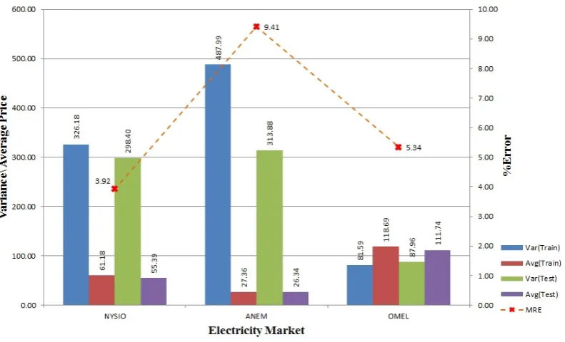
Statistical distributions of the price data have significant effect over the predictions accuracy of the model. In this section we analysis different properties of electricity price data for all three markets. We try to find correlation between data distribution and prediction error. Further, we justify the requirement of independent prediction model for each hour of the day as proposed in our approach. Figures2and3show overall variance and average price for 2004–2006 and 2008–2012 training and testing data for all three electricity market along with average forecasting accuracy. From both figures, we can see that NYISO and ANEM data are of high variance. But when we compare the value with the respective average price, ANEM shows a higher variance in price with a lower average price.
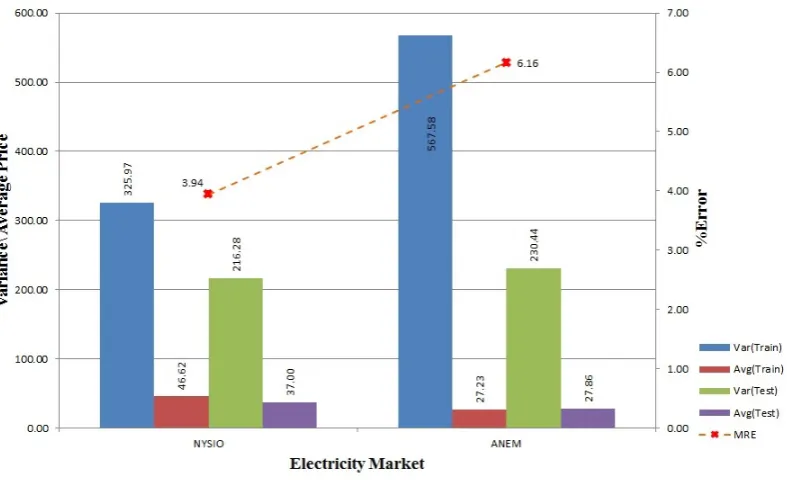
Figure 3.Variance, average, and error in training and testing data for NYISO and ANEM (2008–2012).
Higher variance in price and higher deviation in hourly training and testing data might be the reason for higher error for ANEM’s 2004–2006 dataset as shown in Figure2. From Figure3, we can see for the 2008–2012 dataset, ANEM continues to have higher variance in the training and the testing data, but Figure8shows that the hourly variance deviation between the training and the testing data is less, which helps to lower the forecasting error for ANEM. In Figure6, we can see that the OMEL dataset shows a different response to hourly variance in the dataset. As opposed to NYISO and ANEM, the OMEL 2004–2006 dataset is of lower variance to average price ratio but still its prediction error is higher than that of NYISO. The main cause behind this prediction error is due to presence of few outliers, where the ratio between the maximum the the minimum electricity price is more than 1000 folds. (The data values for the OMEL dataset in Figure2are proportionally adjusted to make them comparable to those of the other markets because, unlike the others, the OMEL market represent electricity price in Euro cent per kWh.)
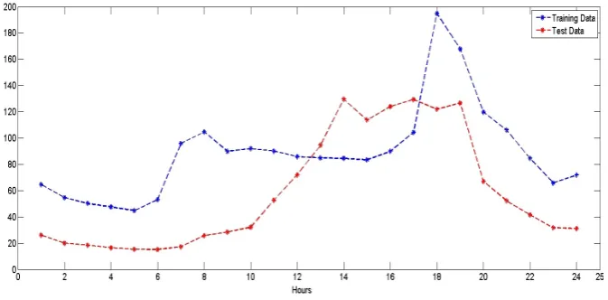
Figure 5.Hourly variance in training and testing data for ANEM (2004–2006).
Figure 6.Hourly variance in training and testing data for OMEL (2004–2006).
Figure 7.Hourly variance in training and testing data for NYISO (2008–2012).
Figure 8.Hourly variance in training and testing data for ANEM (2008–2012).
and6 show the hourly variance in 2004–2006 electricity price data for NYISO, ANEM, and OMEL respectively. Similarly, Figures7and8 show the hourly variance in 2008–2012 electricity prices for NYISO and ANEM respectively. From these 5 figures, we can see that each market exhibits different distribution of data over different hours of the day. For example, if we look into Figure5, we can see that the ANEM 2004–2006 dataset shows price variances ranging from 30 to 1400 AUD/MWh for the training dataset and from 32 to 1950 AUD/MWh for the testing dataset. We can see similar fluctuations in price variances for the NYISO and OMEL datasets as well. These markets are also of different variances in price over hours of the day, but both the training and the testing data follows a similar trend. On the other hand, the ANEM market shows a large difference in the training vs. testing curves for the 2004–2006 dataset but somewhat more consistent curves for the 2008–2012 dataset.
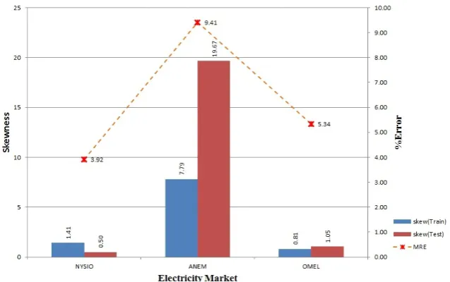
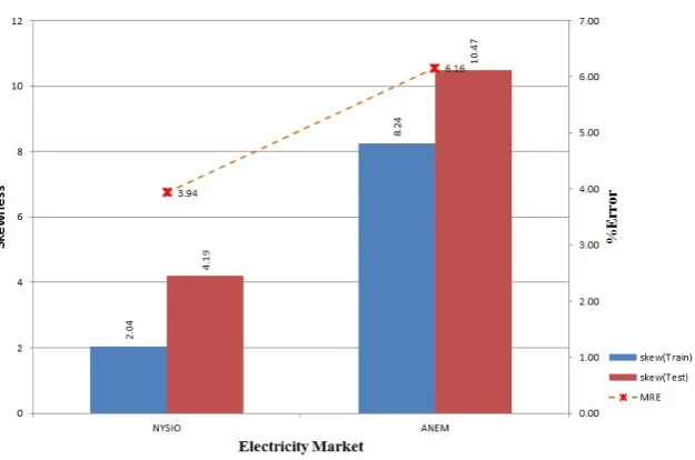
From Figure9, we can see that the ANEM 2004–2006 dataset exhibits high skewness along with higher forecasting error when compared to NYISO and OMEL. This high skewness continues in the ANEM 2008–2012 dataset shown in Figure10.
Figure 10.Skewness in training and testing data for NYISO and ANEM (2008–2012).
From all the above observations, we can infer that electricity markets are of different price distributions which are highly dependent on the hour of the day, with some hours having higher variance in price and some with lower variance. This distribution is further influenced by the deployment of smart grid, where the electricity price depends on various factor like the load, user behavior, demand-response, etc. Under this circumstance, it very difficult to find an approach which can offer consistent performance over different electricity markets. This issue is somehow resolved by our proposed model which provides flexibility on participating algorithms and tries to adapt to the changes in data distribution. Our proposed model captures the variation in price with carefully engineered features and build varying forecasting models separately, one for each hour of the day. The model automatically adjusts itself to certain changes in the environment by evaluating the performance of the model at the end of each day and make necessary adjustments if required.
6.2. Ensemble Model
Two different experiments were performed with different approaches (FWM and VWM) for updating the weights of the participating algorithms. From the results, we can see that the performance of VWM was slightly better than that of FWM. This was because in VWM, the weights are adjusted based on the prediction error, i.e., the change in weight is higher if the difference between the real and the predicted value is higher. Whereas in FWM, changes in weight do not depend upon the level of accuracy of the algorithm, and it just looks at which algorithm performs the best. In VWM, each algorithm is evaluated based on all its previous errors, which is directly correlated to the final prediction accuracy of the model. VWM is better (incurs less error) than FWM by 0.06%–0.18% of MER, 0.03–0.04 of MAE (USD/MWh, AUD/MWh, or EURc/kWh) and 0.05%–0.24% of MAPE. Both approaches show high improvement in accuracy compared to our benchmark method (PSF) and some improvement over our previous work (ANN-only).
unforeseen factors, cause degradation in performance of our ensemble model (both for VWM and FWM). We can see that our model’s performance for few months is below its average performance due to many sharp price increases in those months.
6.3. Comparisons with PSF and ANN-only Methods
To validate the performance of our proposed methods, FWM and VWM, we compared our results with those obtained in other studies found in the literature.
Firstly, we select Pattern Sequence-based Forecasting (PSF) [11] method as our benchmark for comparison. It was shown in experiments that PSF outperformed other contemporary works, namely, ARIMA, naive Bayes, ANN1, WNN (Weighted Nearest Neighbor) [41], STR [42], and mixed model [11]. As testing was performed on the year 2006 data from all three markets in the PSF paper, we also perform the testing on same data and achieve the results shown in Tables2,4, and 3. We can observe that our proposed FWM (VWM in the brackets) forecasts with 1.61% (1.67%) improved accuracy in terms of MER in NYISO dataset. There are improvements (decreases in error)of average MER by 0.35% (1.17%) for ANEM dataset and 0.81% (0.89%) for OMEL dataset. Similar accuracy improvements of FWM/VWM over PSF can be seen for the MAE criterion as well. FWM (VWM in the brackets) offers higher accuracy over PSF in average MAE by USD1.15/MWh (USD1.20/MWh), AUD0.19/MWh (AUD0.05/MWh), EURc0.13/kWh (EURc0.12/kWh) for NYISO, ANEM, and OMEL respectively. Also, we can claim that the forecasting results are more consistent as the standard deviations on both MER and MAE by FWM/VWM are smaller than those by PSF. Thus, without comparing directly with other techniques, we can conjuncture that FWM and VWM will outperform the other standard time-series forecasting methods like ARIMA, naive Bayes, etc.
Secondly, we evaluate the performance with our own recent work using the ANN-only method [12], which was shown to provide higher forecasting accuracy than PSF. For the 2004–2006 datasets, both FWM and VWM provide better results than ANN-only for NYISO. FWM (VWM in the brackets) provides improvements of 0.21% (0.27%) in MER, USD0.12/MWh (USD0.17/MWh) in MAE, and 0.21% (0.25%) in MAPE. For the ANEM dataset, FWM turns out to be inferior to ANN-only by -0.65% MER, -0.11AUD/MWh MAE, and -0.53% MAPE. However, VWM is still better than ANN-only by 0.17% MER, AUD0.03/MWh MAE, and 24% MAPE. For the OMEL dataset, both FWM and VWM are slightly better than or perform equally as ANN-only. The improvements of FWM (VWM in the brackets) for OMEL dataset are 0% (0.08%) MER, EURc0/kWh (EURc0.01/kWh) MAE, and 0.01% (0.14%) MAPE. In terms of S.D., FWM provides smaller S.D. values than ANN-only in 5 out of 9 test cases (i.e., 3 datasets×3 evaluation criteria), and VWM provides smaller S.D. than ANN-only in 6 out of 9 test cases. Similar trends are also observed for the NYISO and ANEM 2008–2012 datasets thus confirming the effectiveness of the proposed VWM and FWM methods.
7. Conclusion
Electricity price forecasting in deregulated electricity market is essential to facilitate the decision making processes of the stakeholders. Although extensive research has been carried out in this field, the accuracy of existing techniques are not consistently high especially in the volatile and complex market conditions. In this paper, we proposed an ensemble-based model using three different algorithm participating for electricity price forecasting. We proposed two different approaches to update the weights of the participating algorithms and select the expert algorithm, whose prediction will be used as the final prediction of the model. We performed comparative experimental studies to benchmark our proposed model with a recent highly-regarded study named PSF, which has been proved to be superior to many other existing methods, as well as with our own previous work using
1 This ANN implementation is distinct from our previous work (ANN-only) [12] because of different feature engineering
a single ANN regressor only. We run experiments of our model on 2006 to 2012 data from 3 different electricity markets. Experimental results demonstrated that our model outperforms both PSF and ANN-only approaches, and it can forecast robustly and accurately even with various datasets over various time periods.
However, we believe that there are still rooms for improvement, and we plan to carry out the following tasks in our future works.
• Application of the model to other electricity markets.
• Inclusion of other exogenous features such as oil/gas prices and method of electricity generation, etc.
• Incorporation of features to model dynamics associated with the smart grid like demand response and load balancing.
• Development of better weighting schemes to further improve the accuracy.
Author Contributions:Author Contributions
BN designed and developed the system, performed the experiments, and wrote the initial draft of the paper. WLW and ZA supervised the project, provided technical guidelines and insights, and carried out the final write-up of the paper.
Conflicts of Interest:Conflicts of Interest
The authors declare no conflict of interest.
References
1. Simmhan, Y.; Agarwal, V.; Aman, S.; Kumbhare, A.; Natarajan, S.; Rajguru, N.; Robinson, I.; Stevens, S.; Yin, W.; Zhou, Q.; Prasanna, V. Adaptive energy forecasting and information diffusion for smart power grids. Proceedings of the 2012 IEEE International Scalable Computing Challenge (SCALE), 2012, pp. 1–4. 2. Shawkat Ali, A.B.M.; Zaid, S. Demand forecasting in smart grid. In Smart Grids: Opportunities,
Developments, and Trends; Springer, 2013; pp. 135–150.
3. Shen, W.; Babushkin, V.; Aung, Z.; Woon, W.L. An ensemble model for day-ahead electricity demand time series forecasting. Proceedings of the 4th ACM Conference on Future Energy Systems (e-Energy), 2013, pp. 51–62.
4. Jurado, S.; Nebot, A.; Mugica, F.; Avellana, N. Hybrid methodologies for electricity load forecasting: Entropy-based feature selection with machine learning and soft computing techniques. Energy 2015, 86, 276–291.
5. Papaioannou, G.P.; Dikaiakos, C.; Dramountanis, A.; Papaioannou, P.G. Analysis and modeling for short- to medium-term load forecasting using a hybrid manifold learning principal component model and comparison with classical statistical models (SARIMAX, Exponential Smoothing) and artificial intelligence models (ANN, SVM): The case of Greek electricity market.Energies2016,9, 635.
6. Jakasa, T.; Androcec, I.; Sprcic, P. Electricity price forecasting — ARIMA model approach. Proceedings of the 8th International Conference on the European Energy Market (EEM), 2011, pp. 222–225.
7. Li, G.; Liu, C.C.; Lawarree, J.; Gallanti, M.; Venturini, A. State-of-the-art of electricity price forecasting. Proceesings of the 2005 CIGRE/IEEE PES International Symposium, 2005, pp. 110–119.
8. Aggarwal, S.K.; Saini, L.M.; Kumar, A. Electricity price forecasting in deregulated markets: A review and evaluation. International Journal of Electrical Power and Energy Systems2009,31, 13–22.
9. Weron, R. Electricity price forecasting: A review of the state-of-the-art with a look into the future. International Journal of Forecasting2014,30, 1030–1081.
10. Martínez-Álvarez, F.; Troncoso, A.; Asencio-Cortés, G.; Riquelme, J.C. A survey on data mining techniques applied to electricity-related time series forecasting. Energies2015,8, 13162–13193.
11. Martínez-Álvarez, F.; Troncoso, A.; Riquelme, J.C.; Aguilar-Ruiz, J.S. Energy time series forecasting based on pattern sequence similarity. IEEE Transactions on Knowledge and Data Engineering2011,23, 1230–1243. 12. Neupane, B.; Perera, K.S.; Aung, Z.; Woon, W.L. Artificial neural network-based electricity price
13. NYISO: New York Independent System Operator. http://www.nyiso.com/public/markets_operations/ market_data/pricing_data/index.jsp.
14. ANEM: Australias National Electricity Market. http://www.aemo.com.au/en/Electricity/NEM-Data/ Price-and-Demand-Data-Sets.
15. OMEL: Spanish Electricity Price Market Operator. http://www.omel.es.
16. Yu, L.; Wang, S.; Lai, K.K. An EMD-based neural network ensemble learning model for world crude oil spot price forecasting. InSoft Computing Applications in Business; 2008; Vol. 230,Studies in Fuzziness and Soft Computing, pp. 261–271.
17. Zhu, B. A novel multiscale ensemble carbon price prediction model integrating empirical mode decomposition, genetic algorithm and artificial neural network.Energies2012,5, 355–370.
18. Contreras, J.; Espinola, R.; Nogales, F.J.; Conejo, A.J. ARIMA models to predict next-day electricity prices. IEEE Transactions on Power Systems2003,18, 1014–1020.
19. Box, G.E.P.; Jenkins, G.M.Time Series Analysis: Forecasting and Control, 3rd ed.; Prentice Hall, 1994. 20. Tan, Z.; Zhang, J.; Wang, J.; Xu, J. Day-ahead electricity price forecasting using wavelet transform
combined with ARIMA and GARCH models. Applied Energy2010,87, 3606–3610.
21. Voronin, S.; Partanen, J. Price forecasting in the day-ahead energy market by an iterative method with separate normal price and price spike frameworks. Energies2013,6, 5897–5920.
22. Singh, N.K.; Tripathy, M.; Singh, A.K. A radial basis function neural network approach for multi-hour short term load-price forecasting with type of day parameter. Proceedings of the 6th IEEE International Conference on Industrial and Information Systems (ICIIS), 2011, pp. 316–321.
23. Singhal, D.; Swarup, K.S. Electricity price forecasting using artificial neural networks.International Journal of Electrical Power and Energy Systems2011,33, 550–555.
24. Lin, W.M.; Gow, H.J.; Tsai, M.T. Electricity price forecasting using enhanced probability neural network. Energy Conversion and Management2010,51, 2707–2714.
25. Gong, D.S.; Che, J.X.; Wang, J.Z.; Liang, J.Z. Short-term electricity price forecasting based on novel SVM using artificial fish swarm algorithm under deregulated power. Proceedings of the 2nd International Symposium on Intelligent Information Technology Application (IITA), 2008, Vol. 1, pp. 85–89.
26. Sansom, D.C.; Downs, T.; Saha, T.K. Support vector machine based electricity price forecasting for electricity markets utilising projected assessment of system adequacy data. Proceedings of the 6th International Power Engineering Conference (IPEC), 2003, pp. 783–788.
27. He, D.; Chen, W.P. A real-time electricity price forecasting based on the spike clustering analysis. Proceedings of the 2016 IEEE/PES Transmission and Distribution Conference and Exposition (T&D), 2016, pp. 1–5.
28. Hong, Y.Y.; Wu, C.P. Day-ahead electricity price forecasting using a hybrid principal component analysis network. Energies2012,5, 4711–4725.
29. Mori, H.; Itagaki, T. A fuzzy Inference net approach to electricity price forecasting. Proceedings of the 54th IEEE International Midwest Symposium on Circuits and Systems (MWSCAS), 2011, pp. 1–4. 30. Kintsakis, A.M.; Chrysopoulos, A.; Mitkas, P.A. Agent-based short-term load and price forecasting using
a parallel implementation of an adaptive PSO trained local linear wavelet neural network. Proceedings of the 12th International Conference on the European Energy Market (EEM), 2015, pp. 1–5.
31. Zhou, Z.Ensemble Methods: Foundations and Algorithms; Chapman and Hall/CRC, 2012. 32. Heaton, J.Introduction to the Math of Neural Networks; Heaton Research, Inc., 2012.
33. Smola, A.J.; Schölkopf, B. A tutorial on support vector regression. Statistics and Computing 2004, 14, 199–222.
34. Breiman, L. Random forests. Machine Learning2001,45, 5–32.
35. Ditzler, G.; Roveri, M.; Alippi, C.; Polikar, R. Learning in nonstationary environments: A survey. IEEE Computational Intelligence Magazine2015,10, 12–25.
36. Azadeh, A.; Ghadrei, S.F.; Nokhandan, B. One day-ahead price forecasting for electricity market of Iran using combined time series and neural network model. Proceedings of the 2009 IEEE Workshop on Hybrid Intelligent Models and Applications (HIMA), 2009, pp. 44–47.
37. Weather Underground: Weather Forecasts and Reports. https://www.wunderground.com/. 38. Matlab - Matworks. www.mathworks.com/products/matlab/.
40. Hall, M.; Frank, E.; Holmes, G.; Pfahringer, B.; Reutemann, P.; Witten, I.H. The WEKA data mining software: An update. SIGKDD Explorations Newsletter2009,11, 10–18.
41. Lora, A.T.; Santos, J.M.R.; Exposito, A.G.; Ramos, J.L.M.; Santos, J.C.R. Electricity market price forecasting based on weighted nearest neighbors techniques. IEEE Transactions on Power Systems2007,22, 1294–1301. 42. Chen, J.; Deng, S.J.; Huo, X. Electricity price curve modeling and forecasting by manifold learning. IEEE
Transactions on Power Systems2008,23, 877–888.
c