Progress in the improved lattice calculation of direct
CP-violation in the Standard Model
ChristopherKelly1
1Columbia University, 538 W 120th St., New York NY 10027
Abstract. We discuss the ongoing effort by the RBC & UKQCD collaborations to
im-prove our lattice calculation of the measure of Standard Model direct CP violation,,
with physical kinematics. We present our progress in decreasing the (dominant) statisti-cal error and discuss other related activities aimed at reducing the systematic errors.
1 Introduction
The leading explanation for the dominance of matter over antimatter in the Universe, baryogenesis, requires the breaking of the CP-symmetry. While such a breaking occurs in the Standard Model, its size appears insufficient to account for the disparity, suggesting new Beyond the Standard Model
sources of CP-violation (CPV) have yet to be discovered.
A particularly attractive avenue for searching for such physics is in the direct CP-violation occur-ing in the decays ofKLinto two pions, which is heavily suppressed in the Standard Model. This was
discovered during the late 1990s with the following result:
Re(/)≈16
1−ηη00
±
2
=16.6(2.3)×10−4,
where and are the measures of direct and indirect CPV, respectively, and ηi j = A(KL →
πiπj)/A(KS → πiπj). Unfortunately the use of this ground-breaking discovery in the search for new
physics has until recently been hampered by the lack of a corresponding, reliable Standard Model calculation, due to the processes involved receiving large contributions from non-perturbative QCD effects, thus preventing the accurate use of perturbation theory.
In 2015 the RBC & UKQCD collaborations published [1] the first direct calculation ofin the
Standard Model using lattice QCD via the isospin-definite amplitudesAI =K→(ππ)I, whereIrefers
to the isospin quantum number of the finalππstate. These amplitudes are computed as
AI =FG√F
2V
∗
usVud[zi(µ)+τyi(µ)]Zi j(µ)(ππ)I|Qj(µ)|K, (1)
whereFis the Lellouch-Lüscher factor [2] that represents the finite-volume correction to the decay amplitude,zandyare c-number Wilson coefficients,τ = −Vts∗Vtd/VudVus∗,Vi j are CKM matrix
relating the bare lattice operators to MS operators normalized at the scaleµ, thereby matching the
scheme used in the calculation of the Wilson coefficients.
We obatained the following result:
Re
ε ε
= Re
i
ωei(δ2−δ0) √
2ε
ImA
2
ReA2 −
ImA0
ReA0
= 1.38(5.15)(4.59)×10−4, (2)
where the errors are statistical and systematic, respectively. HereδIare the s-waveππ-scattering phase
shifts andω = ReA2/ReA0. This result has roughly three times larger errors than the experimental
value, and agrees at the 2.1σlevel. However the possibility of a tension has generated much excite-ment within the physics community and has provided strong motivation for improving the calculation. Since the aforementioned publication we have pursued a programme of substantially improving the errors on our calculation, and in this document we provide an update on our progress.
2 Brief review of lattice calculation of
A
0The errors on our result are dominated by those ofA0. We begin by briefly reviewing the details
of the calculation of this quantity. We performed our measurements on 216 lattice configurations generated with the Möbius domain wall fermion action withLs =12 and the Iwasaki+DSDR gauge
action atβ=2.13. Our pion masses are physical, measuringmπ =143.1(2.0) MeV, and the inverse lattice spacing is a somewhat coarse 1.378(7) GeV. With this coarse lattice spacing we obtain a large, (4.6 fm)3 spatial volume – vital for controlling finite-volume effects – while keeping the number
of lattice sites to a computationally tractable number, at the cost of increased discretization errors. Here the Iwasaki+DSDR action heavily suppresses the ‘dislocations’ (tears) in the gauge field that
contribute strongly to the residual chiral symmetry breaking on coarse lattices, allowing us to simulate with a small fifth-dimensional extent.
On the lattice, the ground-state of theI=0ππsystem (after subtracting the vacuum contribution),
comprises two pions at rest, and thus has an energy of∼280 MeV, much smaller than the kaon mass of∼500 MeV. In order to ensure that the K → ππdecay is energy conserving we therefore use
G-parity boundary conditions (BCs) [3–5] on the quarks in all three spatial directions; these boundary conditions make the pion states antiperiodic in the spatial directions, thereby increasing their ground-state momentum from zero toπ/L, whereL=32 is the spatial box size. With this choice of volume
and boundary condition we obtained a close match between ourππenergy ofEI=0
ππ =498(11) MeV and our kaon mass ofmK =490.6(2.4) MeV. Unfortunately the presence of disconnected diagrams
requires degeneracy between the valence and sea spectra in order to satisfy unitarity, and as such we must generate new, custom gauge configurations with G-parity BCs.
The measurements were performed using all-to-all (A2A) propagators [6], whereby an approxi-mation to the propagator is generated by combining the low-mode contribution obtained using 900 exact eigenmodes of the Dirac operator (computed using the Lanczos algorithm), and a stochastic approximation to the high-mode contribution. Aside from the ability to maximally sample the source, sink and operator locations, this approach allows us to tune the spatial structure of our sources/sinks to
maximize the overlap with the desired state and, in the case of theππstate, minimize the contribution
of the vacuum; in our case we use 1s hydrogen-wavefunction sources with a radius of two lattice sites. The renormalization matrices are computed without using perturbative QCD at the hadronic scale through the use of an intermediate, non-perturbative ‘regularization-invariant momentum scheme’ with symmetric kinematics (RI-SMOM) [7, 8], the basis of which comprises the 7 independent dimension-6 four-quark operatorsQ
relating the bare lattice operators to MS operators normalized at the scaleµ, thereby matching the
scheme used in the calculation of the Wilson coefficients.
We obatained the following result:
Re ε ε = Re i
ωei(δ2−δ0) √
2ε
ImA
2
ReA2 −
ImA0
ReA0
= 1.38(5.15)(4.59)×10−4, (2)
where the errors are statistical and systematic, respectively. HereδIare the s-waveππ-scattering phase
shifts andω = ReA2/ReA0. This result has roughly three times larger errors than the experimental
value, and agrees at the 2.1σlevel. However the possibility of a tension has generated much excite-ment within the physics community and has provided strong motivation for improving the calculation. Since the aforementioned publication we have pursued a programme of substantially improving the errors on our calculation, and in this document we provide an update on our progress.
2 Brief review of lattice calculation of
A
0The errors on our result are dominated by those ofA0. We begin by briefly reviewing the details
of the calculation of this quantity. We performed our measurements on 216 lattice configurations generated with the Möbius domain wall fermion action withLs =12 and the Iwasaki+DSDR gauge
action atβ=2.13. Our pion masses are physical, measuringmπ =143.1(2.0) MeV, and the inverse lattice spacing is a somewhat coarse 1.378(7) GeV. With this coarse lattice spacing we obtain a large, (4.6 fm)3 spatial volume – vital for controlling finite-volume effects – while keeping the number
of lattice sites to a computationally tractable number, at the cost of increased discretization errors. Here the Iwasaki+DSDR action heavily suppresses the ‘dislocations’ (tears) in the gauge field that
contribute strongly to the residual chiral symmetry breaking on coarse lattices, allowing us to simulate with a small fifth-dimensional extent.
On the lattice, the ground-state of theI=0ππsystem (after subtracting the vacuum contribution),
comprises two pions at rest, and thus has an energy of∼280 MeV, much smaller than the kaon mass of∼500 MeV. In order to ensure that the K → ππdecay is energy conserving we therefore use
G-parity boundary conditions (BCs) [3–5] on the quarks in all three spatial directions; these boundary conditions make the pion states antiperiodic in the spatial directions, thereby increasing their ground-state momentum from zero toπ/L, whereL =32 is the spatial box size. With this choice of volume
and boundary condition we obtained a close match between ourππenergy ofEI=0
ππ =498(11) MeV and our kaon mass ofmK =490.6(2.4) MeV. Unfortunately the presence of disconnected diagrams
requires degeneracy between the valence and sea spectra in order to satisfy unitarity, and as such we must generate new, custom gauge configurations with G-parity BCs.
The measurements were performed using all-to-all (A2A) propagators [6], whereby an approxi-mation to the propagator is generated by combining the low-mode contribution obtained using 900 exact eigenmodes of the Dirac operator (computed using the Lanczos algorithm), and a stochastic approximation to the high-mode contribution. Aside from the ability to maximally sample the source, sink and operator locations, this approach allows us to tune the spatial structure of our sources/sinks to
maximize the overlap with the desired state and, in the case of theππstate, minimize the contribution
of the vacuum; in our case we use 1s hydrogen-wavefunction sources with a radius of two lattice sites. The renormalization matrices are computed without using perturbative QCD at the hadronic scale through the use of an intermediate, non-perturbative ‘regularization-invariant momentum scheme’ with symmetric kinematics (RI-SMOM) [7, 8], the basis of which comprises the 7 independent dimension-6 four-quark operatorsQ
1−Q7 and all relevant dimension-3 and 4 operators. Since our
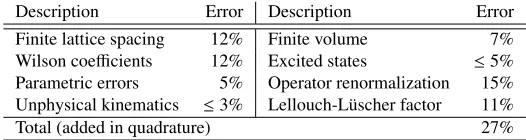
Description Error Description Error Finite lattice spacing 12% Finite volume 7% Wilson coefficients 12% Excited states ≤5%
Parametric errors 5% Operator renormalization 15% Unphysical kinematics ≤3% Lellouch-Lüscher factor 11% Total (added in quadrature) 27%
Table 1: Representative, fractional systematic errors for the individual operator contributions to Re(A0) and Im(A0).
publication we have extended the basis [9] to include the single two-quark dimension-6 operatorG1
that mixes atO(α). We neglect two other dimension-6 operators that mix atO(α2), and all
dimension-5 operators that come with a coefficient of the quark mass as these are expected to be small. We use
this scheme to run to a high energy scale at which continuum perturbation theory can be reliably used to match to MS. In our case, however, the limit of the lattice cutoffforced us to to use a rather low
scale of 1.531 GeV for this matching, resulting in larger perturbative truncation errors. We obtained the following values for the real and imaginary parts ofA0:
Re(A0)=4.66(1.00)(1.26)×10−7GeV and Im(A0)=−1.90(1.23)(1.08)×10−11GeV, (3)
where the errors are statistical and systematic, respectively; for this calculation these errors are roughly comparable. The breakdown of the systematic errors is reproduced in Table1. The most significant contributions are due to the perturbative truncation errors associated with the Wilson coefficients and
with the RI-SMOM→ MS matching. The former is large mainly due to the use of perturbation theory in the three-to-four flavor matching, and the latter due to our low renormalization scale. The discretization error is also comparable in size.
In the remainder of this document we describe our ongoing consecutive efforts to reduce both the
systematic and statistical errors.
3 Reduction of statistical errors
Our goal was to increase the our statistics by a factor of four, toO(900) measurements, thereby reduc-ing the statistical error by 2×, by the end of 2017. We describe this programme and the improvements in more detail below.
3.1 Configuration generation
3.1.1 Algorithmic improvements
Simulating with G-parity BCs is computationally expensive due to a necessary factor of two in the cost of applying the explicitly two-flavor Dirac operator, and also the requirement, for a 2+1 flavor
calculation, to take the square-root of the light-quark action det(D†D) (and a fourth-root for the strange
quarks), which here represents the action offourindependent flavors. The use ofD†D, whereDis
the Dirac operator, is to ensure the matrix is Hermitian and positive-definite, a requirement of the conjugate gradient (CG) algorithm.
The rooting is performed using the RHMC algorithm [10], for which multi-shift CG is typically used to efficiently evaluate the terms of the rational approximation. This algorithm is more expensive
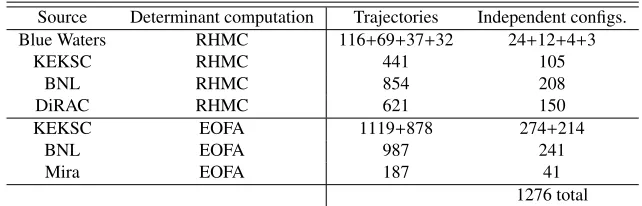
Source Determinant computation Trajectories Independent configs. Blue Waters RHMC 116+69+37+32 24+12+4+3
KEKSC RHMC 441 105
BNL RHMC 854 208
DiRAC RHMC 621 150
KEKSC EOFA 1119+878 274+214
BNL EOFA 987 241
Mira EOFA 187 41
1276 total
Table 2: A summary of our configuration generation, not including the original 216 configurations. In the “trajectories” column, numbers presented in sum indicate the respective sizes of independent streams running on that same machine. Independent configurations are separated by 4 MD time units, and 20 MD time units are discarded at the start of each stream.
large eigenvalue range and the apparent intolerance of the algorithm to finite-precision errors forced us to use a large number of poles with relatively tight stopping conditions. The additional costs also hamper our ability to use the Hasenbusch preconditioning scheme to tune the molecular dynamics, thus requiring smaller MD time steps.
Recently we have been able to bypass the use of RHMC for the light quarks entirely by imple-menting with high efficiency [11] the “exact one-flavor action” (EOFA) [12], a variant of the domain
wall fermion action that represents the determinant of a single quark flavor (two flavors in our case) without the need for rooting. This is achieved by carefully factorizing the domain wall determinant into two pieces that are each Hermitian and positive-definite, allowing them to be inverted directly using regular CG. This technique opened up the ability to further tune the evolution by introducing more Hasenbusch steps, and allowed us to make full use of mixed-precision CG. We could formerly generate one trajectory every 7.7 hours on 512-nodes of BG/Q using the RHMC-based approach;
with EOFA and careful tuning we were able to achieve a factor of 4.2×speed-up, reducing the time to generate a trajectory to just 1.8 hours on the same machine [11].
3.1.2 Summary of configuration status
While configuration generation by Markov chain Monte Carlo is necessarily a sequential process, we were able to significantly increase the rate of configuration generation by running multiple inde-pendent streams starting from widely separated points of our original, thermalized ensemble. Our previous results suggest an autocorrelation time of4 MD time units, therefore for each stream we discard the first 20 trajectories (5 autocorrelation lengths) to ensure independent ensembles.
We performed the bulk of our generation using the BG/Q machines ‘KEKSC’ at KEK, Japan;
‘DiRAC’ at Edinburgh, UK; the ‘Mira’ machine at ALCF; and the BG/Q machines at RBRC/BNL.
Here we utilize the CPS framework with the Bagel/BFM library [13] for highly-optimized BG/Q
solvers. We also made some use of the Blue Waters (AMD ‘Interlagos’ processors) using CPS atop the Grid framework [14] for optimal kernel performance.
In Table2 we give the status of configuration generation at the time of writing. Including the original 216 configurations, theO(1500) resulting configurations represents a factor of seven increase in statistics over the original calculation. This exceeds our original target of 900 configurations by a significant margin. At this point we have halted further configuration generation in favor of performing measurements, which, due to the above improvements are now lagging significantly behind.
3.2 Measurements
Since the time of our original publication we have completely refactored our CPS-based measurement code and have implemented a number of strategies to improve performance on a variety of architec-tures, with particular emphasis on the BG/Q and Intel “Knight’s Landing” (KNL) machines. The
measurements comprise three stages: the generation of the eigenvectors using the Lanczos procedure; theO(1500) deflated Dirac operator inversions associated with the (time-spin-color-flavor diluted) high-mode approximation; and finally the A2A contractions themselves.
3.2.1 Algorithmic improvements
For the contractions we have implemented a number of improvements including:
• Spatial decomposition of the CPS fermion fields across the SIMD lanes allowing optimal use of QPX intrinsics on BG/Q and AVX512 intrinsics on Intel KNL.
• A hand-coded AVX512 assembly kernel for the most computationally expensive part of the contrac-tions, which achieves over 400 Gflops double-precision performance on KNL. We have also added Grid-based intrinsics kernels for other architectures including BG/Q, resulting in a significant
per-formance gain.
• Optimized distribution of work over nodes and threads for underlying matrix operations and use of highly-tuned MKL, ATLAS BLAS libraries where appropriate.
• An optimized parallel FFT that divides the lattice into one-dimensional strips and spreads this work over nodes and threads to maximize parallelization.
• A flexible structure for adapting to memory constraints, particularly on the BG/Q machines,
includ-ing a distributed memory model for storinclud-ing intermediate data with optional temporary disk storage to make use of burst buffers where available.
As a result of these changes we were able to add additional quantities to our measurement pro-gramme while keeping the total measurement time the same on 512-nodes of BG/Q. We now measure
with a second source smearing – a 2s hydrogen-wavefunction form with a radius of 2 – and also com-pute theσ → σandσ → ππmatrix elements, whereσis a scalar operator with vacuum quantum numbers. As we discuss below, these will provide additional data in theππtwo-point andK → ππ
three-point calculations as well as a better handle on excited states.
We have also added the option to replace the Lanczos and CG implementations with those in the Grid framework, allowing us to perform highly optimized measurements on other architectures. Within Grid we have implemented several improvements, including a hand-coded intrinsics-based G-parity kernel implementation achieving 330 Gflops single-precision performance on KNL (single-node), and an implementation of the mixed-precision ‘reliable-update’ CG approach [15] with half-precision communications for the majority of the iterations to maximize the use of limited network bandwidth. These improvements have enabled us to efficiently perform a large number of
measure-ments on the Cori I (Intel ‘Haswell’) and Cori II (KNL) machines at NERSC.
3.2.2 Status of measurements
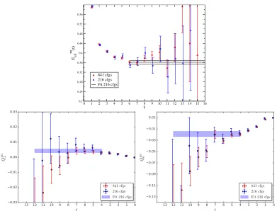
At the time of writing we have performed 774 measurements, not including the original 216; in total roughly 2/3 of the way towards our goal. As a demonstration of our progress, in Figure1we show
the results of increasing the number of measurements to 841 configurations from the original 216 for
ππeffective energy as well as theQ2 andQ6 matrix elements, which are the leading contributors to
the real and imaginary parts ofA0, respectively. We observe a 2×reduction in the statistical errors
0 1 2 3 4 5 6 7 8 9 10 11 12 13 14 15 16
t
0.2 0.24 0.28 0.32 0.36 0.4 0.44 0.48 0.52 0.56
Eeff
ππ
(t)
841 cfgs 216 cfgs Fit 216 cfgs
Figure 1: Theππeffective energy (top) and the lattice matrix elementsQ2(lower-left) andQ6 (lower-right) for 216 configurations and 841 configurations, overlaid by the fit to the former.
4 Improvements in systematic errors
4.0.1 Renormalization and Wilson coefficients
TheO(15%) errors on the renormalization arise due to the low, 1.531 GeV scale at which perturbation theory is applied to match between RI-SMOM and MS. Since publication we have utilized step-scaling to increase the scale to 2.29 GeV, and have also included the two-quark, dimension-6 operator G1that mixes atO(α), for which the effects are at the percent-scale as expected. These improvements were reported on in Ref. [16], in which we demonstrated a reduction of the renormalization systematic to 8% (preliminary), along with an improved procedure for determining the error itself.
We do not expect a similar improvement in the error on the Wilson coefficients from increasing the scale because the dominant contribution to the error arises from the use of perturbation theory to cross the charm threshold at 1.29 GeV. In order to address this issue without performing a full four-flavor calculation of the matrix elements, it is necessary to non-perturbatively match across this threshold, which requires the computation of non-perturbative renormalization factors at scales much lower than the charm scale. As RI-SMOM is a gauge-fixed scheme there is an enlarged set of gauge-noninvariant operators that mix at higher orders ofα, and as such these schemes may become unreliable at such
low scales. To avoid this issue we are investigating the use of the gauge-invariant position space renormalization scheme, and results thus far seem promising.
4.0.2 Finite lattice-spacing errors
We estimate that our coarse, 1.38 GeV lattice spacing gives rise toO(12%) discretization effects, which will dominate the error of our forthcoming calculation. Ideally we would address this by repeating the calculation at a finer lattice spacing, but unfortunately the computational cost of such a venture makes it unfeasible with the present generation of computing hardware.
An alternative is to consider a coarserlattice spacing: For other purposes we have generated a (non-G-parity) 243 ×64×24 Möbius DWF ensemble with the Iwasaki+DSDR gauge action at
β=1.633 – corresponding toa−1≈1.0 GeV – and a physical pion mass. This lattice, unintentionally,
has an almost identical physical spatial volume to our 323×64 G-parity ensemble, making it an ideal candidate for a repeat calculation. While this lattice is very coarse compared to a typical lattice calcu-lation, it appears that the Iwasaki+DSDR gauge action has remarkably small discretization errors, at the percent-scale on this 1 GeV ensemble for a variety of quantities [17]. We must of course generate new configurations with G-parity BCs, but the existence of the non-G-parity lattice enables us to eas-ily compute the RI-SMOM renormalization matrices and the lattice spacing without the complications associated with the G-parity BCs (a situation we also took advantage of in our previous calculation).
While further study of the discretization effects on other, more complex quantities such asBKand
A2are underway, we have thermalized an ensemble with G-parity BCs in anticipation of proceeding with this calculation.
4.0.3 Resolving the “ππpuzzle”
Our previous result for theI = 0ππscattering phase shift, computed as part of theA0 calculation, isδ0=23.8(4.9)(1.2)◦[1], where the errors are statistical and systematic, respectively. This value is
somewhat lower than the value of 38.3(1.3)◦[18,19] obtained by combining experimental data with
the Roy equations. In order to match this phase shift, ourππenergy would need to be∼470 MeV as opposed to the 498(11) MeV measured value.
To address this issue, along with the increased statistics we now measure pion operators with a 2s hydrogen-wavefunction smearing and also compute theσ→σandσ→ππtwo-point functions.
In the continuum theσis a broad resonance of theI =0ππsystem, but on the lattice it is simply
a state that mixes with theππ; the eigenstate of the finite volume QCD Hamiltonian that we refer to
as the “ππ” is therefore more precisely a linear superposition of these two states. While the finite-volume dynamics of this state in the scattering and decays are completely captured by the Lüscher and Lellouch-Lüscher formalisms, respectively, studying correlation functions involving this operator provides more handles on theππsystem with differing excited-state contributions, and therefore offers not just an improvement in statistics on the ground-state energy but also a greater ability to study the spectrum of nearby states, particularly if coupled with the variational method [20]. This will help us to resolve whether our appparently too-largeππenergy is due to contamination from a nearby excited state (although such a state would be incompatible with phenomenology).
4.0.4 Other related, future projects
We have also initiated a number of related long-term projects. One such is the forthcoming calculation of theI = 0 ππenergy using traditional periodic boundary conditions and modern, multi-operator
techniques to extract the excited states. We are also examining the possibility of computingK →
5 Conclusions
In these proceedings we have detailed our progress in the improved calculation ofA0, and therefore
, on the lattice. We report significant progress towards a seven-fold increase in statistics over our initial calculation, with the majority of the work having been completed at the time of writing.
We also discussed a number of programmes to improve the systematic errors, including the ad-dition of newππoperators to better resolve the ground-state energy; a factor of 2×reduction in the renormalization systematic as a result of step-scaling to a higher energy scale; and the inclusion of the G1operator in the renormalization. In addition we outlined our plan for a calculation ofA0with a
sec-ond, coarser lattice spacing in order to better constrain the discretization errors. Finally we mentioned several longer-term projects such as computing the 3→ 4 flavor matching non-perturbatively using position-space NPR; studying the effects of electromagnetism and isospin breaking; and a calculation
of theππenergy using periodic boundary conditions and multi-operator methods.
It is our intention to publish new results forA0andin early 2018.
References
[1] Z. Bai et al. (RBC, UKQCD), Phys. Rev. Lett.115, 212001 (2015),1505.07863 [2] L. Lellouch, M. Luscher, Commun. Math. Phys.219, 31 (2001),hep-lat/0003023 [3] U.J. Wiese, Nucl. Phys.B375, 45 (1992)
[4] C.h. Kim, N.H. Christ, Nucl. Phys. Proc. Suppl. 119, 365 (2003), [,365(2002)], hep-lat/0210003
[5] C. Kelly (RBC, UKQCD), PoSLATTICE2012, 130 (2012)
[6] J. Foley, K. Jimmy Juge, A. O’Cais, M. Peardon, S.M. Ryan, J.I. Skullerud, Comput. Phys. Commun.172, 145 (2005),hep-lat/0505023
[7] G. Martinelli, C. Pittori, C.T. Sachrajda, M. Testa, A. Vladikas, Nucl. Phys.B445, 81 (1995), hep-lat/9411010
[8] C. Sturm, Y. Aoki, N.H. Christ, T. Izubuchi, C.T.C. Sachrajda, A. Soni, Phys. Rev.D80, 014501 (2009),0901.2599
[9] G. McGlynn (2016),1605.08807
[10] M.A. Clark, A.D. Kennedy, Nucl. Phys. Proc. Suppl. 129, 850 (2004), [,850(2003)], hep-lat/0309084
[11] C. Jung, C. Kelly, R.D. Mawhinney, D.J. Murphy (2017),1706.05843 [12] Y.C. Chen, T.W. Chiu (TWQCD), Phys. Lett.B738, 55 (2014),1403.1683 [13] P.A. Boyle, Comput. Phys. Commun.180, 2739 (2009)
[14] P.A. Boyle, G. Cossu, A. Yamaguchi, A. Portelli, PoSLATTICE2015, 023 (2016) [15] G.L.G. Sleijpen, H.A. van der Vorst, Computing56, 141 (1996)
[16] C. Kelly, PoSLATTICE2016, 308 (2016)
[17] R.D. Mawhinney, EPJ Web Conf.LATTICE2017(2017)
[18] G. Colangelo, J. Gasser, H. Leutwyler, Nucl. Phys.B603, 125 (2001),hep-ph/0103088 [19] G. Colangelo, personal communication
[20] M. Luscher, U. Wolff, Nucl. Phys.B339, 222 (1990)