PAN, FENG Exploring Energy-Time Tradeoff in High Performance Computing. (Under the
direc-tion of Vincent W. Freeh).
Recently, energy has become an important issue in high-performance computing. For
example, low power/energy supercomputers, such as Green Destiny, have been built; the idea is to
increase the energy efficiency of nodes. However, these clusters tend to save energy at the expense
of performance. Our approach is instead to use high-performance cluster nodes with frequency
scalable AMD-64 processors; energy can be saved by scaling down the CPU. Our cluster provides
a different balance of power and performance than low-power machines such as Green Destiny. In
particular, its performance is on par with a Pentium 4-equipped cluster.
This thesis investigates the energy consumption and execution time of a wide range of
applications, both serial and parallel, on a power-scalable cluster. We study via direct measurement
both intra-node and inter-node effects of memory and communication bottlenecks, respectively.
Ad-ditionally, we present a framework for executing a single application in several frequency-voltage
settings. The basic idea is to first divide programs in to phases and then execute a series of
experi-ments, with each phase assigned a prescribed frequency.
Our results show that a power-scalable cluster has the potential to save energy by scaling
the processor down to lower energy levels. Furthermore, we found that for some programs, it is
possible to both consume less energy and execute in less time by increasing number of nodes and
reducing frequency-voltage setting of the nodes. Additionally, we found that our phase detecting
by
Feng Pan
A thesis submitted to the Graduate Faculty of North Carolina State University
in partial satisfaction of the requirements for the Degree of
Master of Science
Department of Computer Science
Raleigh
2005
Approved By:
Dr. Eric Rotenberg Dr. Jun Xu
Dr. Vincent W. Freeh
Biography
Feng Pan is from Dalian, China. He came to United States in 1998. From 1999 to 2003,
he attended Appalachian State University in Boone, NC, where he received Bachelor of Science
degree in both Computer Science and Applied Math. He began graduate study at North Carolina
State University immediately after his undergraduate career. He will receive Master of Science
Contents
List of Figures iv
List of Tables v
1 Introduction 1
1.1 The Case for Power-Aware, High-Performance Computing . . . 3
1.2 Contributions . . . 5
2 Related Work 6
2.1 Server/Desktop Systems . . . 6
2.2 Mobile Systems . . . 7
3 Single-Gear Results 10
3.1 Single-Node Results . . . 12
3.2 Multiple-Node Results . . . 17
4 Multiple-Gear Results 23
4.1 Profile-Directed Technique . . . 23
4.2 Analysis of Results . . . 30
5 Conclusions and Future Work 34
List of Figures
3.1 Aggregate plots of NAS set. . . 12
3.2 Aggregate plots of SPEC INT set. . . 13
3.3 Aggregate plots of SPEC FP set. . . 14
3.4 Best energy-time tradeoff in each set. . . 14
3.5 Worst energy-time tradeoff in each set. . . 15
3.6 OPM vs.betafor all applications on AMD-64. . . 16
3.7 Energy consumption vs execution time for NAS benchmarks on 2, 4, and 8 (or 4 and 9) nodes. . . 18
3.8 Energy consumption vs. execution time for Jacobi iteration on 2, 4, 6, 8, and 10 nodes. 20 3.9 Relative energy vs. time. . . 21
3.10 Synthetic benchmark with high memory pressure. . . 22
4.1 Trace of operations per miss for LU C. . . 24
4.2 Energy consumption vs. execution time for three NAS benchmarks on a single AMD machine. . . 25
4.3 Heuristic for searching solution space. . . 26
4.4 Energy-time plot of many BT runs. . . 28
List of Tables
3.1 Idle and active power for AMD-64. . . 11
3.2 Predicting CPU boundness. . . 15
Chapter 1
Introduction
High-performance computing (HPC) tends to push performance at all costs.
Unfortu-nately, the “last drop” of performance tends to be the most expensive. For example, the last 10%
increase in performance requires a disproportionally large amount of resources. This
performance-at-all-costs policy is only justifiable given infinite resources. An example of nearly infinite resources
is any of the supercomputing centers, which houses large-scale supercomputers. For example, the
ASCI Q machine consumes more than 3 gigawatts [53]. This unchecked energy consumption costs
the government a significant amount of money and wastes natural resources. Moreover, it is unlikely
that supercomputing centers can continue limitless consumption of resources. In particular, energy
consumption—and the resultant heat dissipation—is becoming an important limiting factor.
As a result, lower-power, high performance clusters such as Orion[42], have been
devel-oped to stem the ever-increasing demand for energy. Such systems improve the energy efficiency
of nodes. However, their performance penalty is usually too large to be reasonable for many users.
If performance is the only goal, then one should continue on the current “performance-at-all-costs”
path of HPC architectures. On the other hand, if power is paramount, then one should use a
low-performance architecture that executes more instructions per unit energy.
We believe one should strike a path between these two extremes. We use a
high-perfor-mance microprocessor that has frequency and voltage-scaling. Each frequency provides an
energy-performance point that we call a gear. It is conceptually possible to save energy without an increase
in time because an increase in CPU frequency generally results in a smaller increase in application
increasing frequency also increases CPU stalls—usually waiting for memory or communication.
Consequently, there are opportunities where energy can be saved, without an undue
per-formance penalty, by reducing CPU frequency. On the other hand, for those programs or parts of a
program (because most programs are not uniform) where the time penalty is large, the processors
should be run at the fastest frequency.
This thesis investigates the tradeoff between energy and performance (execution time)
for HPC. We evaluate on a real, small-scale power-scalable cluster. Each node is equipped with a
AMD-64 processor that supports frequency and voltage scaling.
Towards this goal, we analyzed benchmarks, both serial and parallel, to determine the
relationship between voltage and frequency settings and execution time. Our results show that all
of our tests have what we call an energy-time tradeoff, meaning that a decrease in energy is possible
but it comes at the cost of increased time. Not every energy-time tradeoff is desirable, as some offer
little energy savings and large time penalties. However, more than half of these tests show a savings
that is equal to or better than the penalty (e.g., 10% less energy and 10% more time), and some
are much better than that. In particular, we found that on one node, it is possible to use 20% less
energy while increasing time by 3%, with CG. However, with EP there was essentially no savings.
We present a simple metric that predicts this energy-time tradeoff. Additionally, we found that in
some cases one can save energy and time by executing a program on more nodes at a slower gear
rather than on fewer nodes at the fastest gear. We believe this will be important in the future, where
a program running on a cluster may be allowed to generate only a limited amount of heat.
In addition to exploring the energy-time tradeoff by executing entire programs in a single
gear, this thesis also presents a framework for executing a single application in several
frequency-voltage settings. As mentioned above, most programs are not uniform, as a result, certain parts of
a program may have a different energy-time tradeoff and therefore should be run using a different
gear than other parts of the same program. We implement our scheme by first manually dividing
programs into phases based on trace data collected during a profile of the application. If there aren
phases in an application andgpossible gears, there aregnunique solutions, where a solution is an
assignment of a gear to each phase. We present a novel heuristic that searches the space of solutions.
It executes a solution and evaluates the energy-time tradeoff based on a user-defined metric. Based
on the evaluation, it selects the next solution to evaluate. The heuristic terminates when the results
are satisfactory (again based on input from the user or cluster administrator). The heuristic requires
at mostn·g steps to find a “good” solution; however, we have found that in most cases, it takes
Performance results on the NAS suite show that our heuristic finds effective solutions.
Specifically, we find several solutions that use different gears per phase that are superior to any
solution that used a single gear for all phases. For example, for MG, a multiple-gear solution
executes in the same time but consumes 3% less energy then a single-gear solution. This same
multiple-gear solution executes 8% faster than another single-gear while using the same amount of
energy.
1.1
The Case for Power-Aware, High-Performance Computing
Power-aware computing has flourished over the last decade in many areas, especially
mobile devices. However, it has little traction in HPC computing because the HPC community has
vastly different goals than those of mobile users. Because computational scientists are using HPC
to gain maximum performance, many may resist any mechanism that increases execution time.
We believe that a significant subset of HPC programmers will be forced to accept less
performance in order to conserve power. This will occur because the large and growing power
consumption of current clusters at supercomputer centers—which are not immune to economic
pressures—will eventually come to bear on the cluster users. This may manifest itself in
program-mers utilizing lower-power machines such as Green Destiny [42, 53]. Consider the case of Green
Destiny, which is a cluster of Transmeta processors. While it uses less power and energy than a
conventional supercomputer, it also provides much less performance. In particular, Green Destiny
consumes about three times less energy per unit performance than the ASCI Q machine. However,
because Green Destiny uses a slower (and cooler) microprocessor, ASCI Q is about 15 times faster
per node (200 times overall) [53]. A reduction in performance by such a factor surely is
unreason-able from the point of view of many HPC programmers.
We believe that computational scientists would be more likely to consider energy
reduc-tion if we start from a baseline of a high-performance, scalable microprocessor. Then, from there we
attempt to reduce power with only a small performance loss. The emergence of high-performance
scalable microprocessors, such as the AMD-64/Opteron [2], makes this possible. This
micropro-cessor has performance that is on a par with high-end, fixed frequency desktop micropromicropro-cessors, but
its power consumption can be reduced to 25% of the maximum using frequency and voltage
scal-ing [54]. We expect that such power-performance settscal-ings will be commonplace on most high-end
with virtually no performance loss (e.g., mcf and art from the SPEC benchmark set).
Saving Power and Energy with gear Selection
High-performance computing (HPC) applications and machines are inefficient. For
ex-ample, the 2004 Gordon Bell Prize, which is given annually to the application with the greatest
performance, was awarded to one that sustained 46% parallel efficiency [16]. This means that
on average, a microprocessor in a supercomputer executing the world champion application was
blocked and idling more than half of the time. In such a situation, a traditional microprocessor races
forward at full speed to the next blocking point and waits. While blocked, the machine is
consum-ing energy, but not performconsum-ing any useful work. Furthermore, when a program has good parallel
efficiency, it may not be efficient sequentially (e.g., it may stall waiting for the memory subsystem).
As an analogy, consider a car speeding between stop lights. Because a traditional
mi-croprocessor has only one gear, which uses full power and provides the maximum performance,
it must race between metaphorical stop lights. Recently, manufacturers have begun producing
mi-croprocessors with multiple energy gears. With such a microprocessor, a computer can shift into a
reduced power and performance gear so that computation is potentially completed just in time for
the unblocking event—i.e., arriving just as the light turns green.
This method of execution saves energy in two ways. First, (wasted) energy consumed
while waiting is eliminated. Second, a microprocessor uses less energy per operation at lower
en-ergy gears. This is because while performance is linearly proportional to clock frequency, power
consumption is proportional to frequency and voltage squared. Thus, at a slower gear, a
micropro-cessor will consume less energy per operation than at a faster gear [40]. Again, this follows the
analogy of an automobile—it takes less gasoline to travel at 50 MPH for 2 hours than at 100 MPH
for one hour, partly because drag is proportional to velocity squared.
It may appear that node performance should be reduced solely based on its percentage
of idle time, but this not the case. Doing so blindly will likely mean that events that are on the
critical path are delayed, which increases execution time by the amount of that delay. In this paper,
we investigate the tradeoff between energy and performance (execution time). We closely examine
1.2
Contributions
This thesis makes several contributions. First, using NAS and SPEC benchmark suites,
it evaluates the energy and time tradeoff of single node applications on an AMD-64 processor that
is frequency and voltage scalable—i.e., its clock speed and power consumption can be changed
dynamically. Second, it evaluates a real, small-scale power-scalable cluster, which is a cluster
com-posed of AMD-64 processors described above. Using NAS-MPI benchmark suite, we illustrate the
tradeoff between the power-conserving benefits and the time-increasing costs of such a machine.
Third, it introduces a framework for executing a single application in several frequency-voltage
settings, in order to achieve maximum energy efficiency. This is an initial step to an power-aware
operating system infrastructure that is capable of adjusting processor frequency automatically
with-out user intervention.
The rest of this thesis is organized as follows. Chapter 2 describes related work, Next,
Chapters 3 and 4 present single-gear and multiple-gear results, respectively. Finally, Chapter 5
Chapter 2
Related Work
There has been a voluminous amount of research performed in the general area of energy
management. In this section, we describe some of the closely related research. We divide the related
work into two categories: server/desktop systems and mobile systems.
2.1
Server/Desktop Systems
Several researchers have investigated saving energy in server-class systems. The basic
idea is that if there is a large enough cluster of such machines, such as in hosting centers, energy
management can become an issue. In [7], Chase et al. illustrate a method to determine the aggregate
system load and then determine the minimal set of servers that can handle that load. All other servers
are transitioned to a low-energy state. A similar idea leverages work in cluster load balancing to
determine when to turn machines on or off to handle a given load [46, 47]. Elnozahy et al. [15]
investigated the policy in [46] as well as several others in a server farm. Such work shows that
power and energy management are critical for commercial workloads, especially web servers [4,
36]. Additional approaches have been taken to include DVS [14, 51] and request batching [14].
The work in [51] applies real-time techniques to web servers in order to conserve energy while
maintaining quality of service.
Our work differs from most prior research because it focuses on HPC applications and
servicing client requests. On the other hand, an HPC installation exists to speedup an application,
which is often highly regular and predictable. One HPC effort that addresses the memory bottleneck
is given in [29]; however, this is a purely static approach.
In server farms, disk energy consumption is also significant. One study of four energy
conservation schemes concludes that reducing the spindle speed of disks is the only viable option
for server farms [6]. DRPM is a scheme that dynamically modulates the speed of the disk to save
energy [25, 26]. Another approach is to improve cache performance—if many consecutive disk
accesses are cache hits, the disk can be profitably powered down until there is a miss; this is the
approach taken by [60]. An alternative is to use an approach based on inspection of the program
counter [22]; the basic idea is to infer the access pattern based on inspection of the program counter
and shut down the disk accordingly. A final approach is to try to aggregate disk accesses in time. A
compiler/run-time approach using this was designed and implemented in [27], and a prefetching
ap-proach in [44]. Both were designed for mobile systems but can be directly applied to server/desktop
systems.
There are also a few high-performance computing clusters designed with energy in mind.
One is BlueGene/L [1], which uses a “system on a chip” to reduce energy. Another is Green
Destiny [53], which uses low-power Transmeta nodes. A related approach is the Orion Multisystem
machines [42], though these are targeted at desktop users. However, using a low-power processor
sacrifices performance in order to save energy.
This thesis is partly based on our previously published works. A study of single-node
applications can be found in [43], however, it explores energy-time tradeoff in mobile systems. In
[20] we study the energy-time tradeoff in MPI programs. We have also examined the energy saving
potentials by using multiple energy gears in MPI programs [21]. Another member of our research
group has developed techniques for saving power in datacenters in [17] and [18].
2.2
Mobile Systems
There is also a large body of work in saving energy in mobile systems; most of the early
research in energy-aware computing was on these systems. This subsection details some of these
projects.
ECOSystem [59] attempts to implement a power management system without the need
accounting model is implemented, called the currentcy model. The currentcy model attempts to
attribute energy usage to individual applications, as well as to specific components of the machine.
Each application is allocated a certain amount of currentcy, which corresponds to the total energy it
is allowed to consume in each epoch. The system then accounts for where each application spends
its energy using a combination of real-time feedback from the battery and estimation techniques
(re-quired because the information returned from the battery is too coarse grained). While ECOSystem
is an effective framework for power management, it has the undesirable characteristic of assuming
user knowledge of currentcy. It expects users to have a predetermined idea of how much energy
should be used by each application. Therefore, ECOSystem is not transparent, which we believe is
paramount.
The case for a closer relationship between the operating system system and power
man-agement is further explored by Vahdat et al. [52, 13]. This includes a case for treating energy as a
first class resource in operating systems. Perhaps the best endorsement of OS-controlled power
con-sumption comes from the ACPI (Advanced Configuration and Power Interface) standard [9]. It is
an evolution of several existing methods including BIOS power management, the APM (Advanced
Power Management) API, and a smart battery interface.
In general, the goal of the OS is to conserve energy for the entire set of processes. Our
approach differs in that we are concerned with saving energy in a single program.
Individual Devices Many have worked on saving energy in different devices, such as the CPU,
disk, memory, and network. Many modern processor architectures allow different frequency-voltage
settings. This work developed into dynamic voltage scaling (DVS) [19, 24, 45, 48, 31], which has
come to mean the simultaneous changing of clock speed and voltage to reduce power consumption.
Typically, DVS optimizes the energy×delay or energy×delay2[38, 23] product. This creates a
system that more efficiently uses energy, but is still powerful and responsive. In order to do this,
DVS must accurately predict upcoming load. A poor prediction either consumes too much energy
or causes too much delay. In this work, we investigate the relationship between frequency/voltage
and execution time. DVS is used to adjust frequency and voltage in our multi gear tests.
Disk Disks consume a large percentage of energy on some mobile architectures. Many have
studied disk spindown to save energy (e.g., [28, 12, 55, 3, 37]). In general, the idea is to determine
when there is a large time period in which there are no disk requests and transition to a lower energy
Memory and Network In some architectures, individual memory banks and/or network card has
multiple energy states. Work on transitioning these to lower energy states include [10, 35, 8, 33,
58, 57]. The idea is to place data intelligently in banks so that some banks will not be accessed.
In some devices the network card has multiple energy states. One way to save energy is to use the
energy-saving mechanisms defined by 802.11b [8]. One improvement to 802.11b is the Bounded
Slowdown Protocol [33], which uses minimal energy given a desired maximum increase in round
trip time. In addition, Yan et al. [58] leverage TCP to save energy in large file downloads. Finally,
Kravets investigated power-aware mechanisms for end-to-end communication in wireless networks
[34].
The primary distinction between these projects and ours is that energy saving is
typi-cally the primary concern in mobile devices. In HPC applications, performance is still the primary
concern. Energy consumed by memory banks and network cards is important primarily in mobile
devices. However, in desktop or cluster processors, memory energy consumption is relatively small.
Chapter 3
Single-Gear Results
This chapter describes the results of our single-gear experiments (i.e., we do not change
gear during execution of a single application). We studied programs from three different benchmark
sets: NAS, SPEC integer, and SPEC floating point, in our single node tests. The NAS suite is
a popular high-performance computing benchmark, consisting of scientific benchmarks including
application areas such as sorting, spectral transforms, and fluid dynamics. In contrast, the SPEC
integer benchmarks are non-scientific applications that are CPU and/or memory intensive. The
SPEC floating point benchmarks are a mixture of both scientific and non-scientific programs. For
example, mesa and facerec are non-scientific, graphics programs, whereas swim and mgrid are
well-known scientific benchmarks. In our multi-node tests, we studied NAS MPI suite. We used all valid
configurations using up to 9 nodes. Presumably, such mature benchmarks have been thoroughly
analyzed and are well-written (e.g., see [56])—so that they are not unrealistically communication
bound.
This study uses, as a reference example, a cluster of ten nodes, each equipped with a
frequency- and voltage-scalable AMD Athlon-64. All single node tests are run on one of the
identi-cal nodes. We run each program at each available energy gear: 2000 MHz, 1800 MHz, 1600 MHz,
1400 MHz, 1200 MHz, and 800 MHz.1 The voltage, which ranges from 1.5–1.0V, is reduced in
each gear. Each node has 1GB main memory, a 128KB L1 cache (split), and a 512KB L2 cache,
and the nodes are connected by 100Mb/s network. In this thesis, we control the CPU power and
measure overall system energy. This is effective in saving energy because the CPU—a major power
1
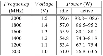
F requency V oltage P ower(W)
(MHz) (V) idle active
2000 1.5 59.6 98.8–108.6
1800 1.4 57.0 86.5–95.2
1600 1.3 55.9 80.1–88.1
1400 1.2 54.8 74.3–81.9
1200 1.1 53.4 67.1–75.4
800 1.0 51.0 56.8–63.5
Table 3.1: Idle and active power for AMD-64.
consumer—uses less power. According to datasheet, the Athlon CPU used in this study consumes
up to 89W with all components fully active[2]. However, given that the maximum system power
we measured is 109W, the CPU must not reach this level in our tests.
For each program we measure execution time and energy consumed for an application at
a range of energy gears. Execution time is elapsed wall clock time. The energy consumed by the
entire system is measured by a WattsUp pro meter[39] attached to each system at the wall outlet
to determine the instantaneous power (in Watts). This value is integrated over time to determine
the energy used. Because we attach a meter to each node, for multi-node tests, the total energy
consumption by all systems can be easily and accurately obtained by calculating the sum of each
individual node’s energy consumption.
Table 3.1 shows idle power and active power ranges for all gears of AMD-64. The active
power ranges are determined using single-node data collected in Chapter 3. The idle power is
determined with CPU in HALT (C1) state. Currently in Linux, CPU enters HALT state when the
operating system determines that the system is idle. We can see that the difference in active power
consumption between highest and lowest frequencies is about 40%, while the difference in idle
power is less than 10%. Thus there is a small benefit to reduce gear before entering the HALT state.
This chapter is divided in to two parts. First, it shows results on a single node. This
section shows the energy-time tradeoff due to the memory bottleneck. Next, it describes time and
energy results on multiple nodes. This section shows the effect of the communication bottleneck as
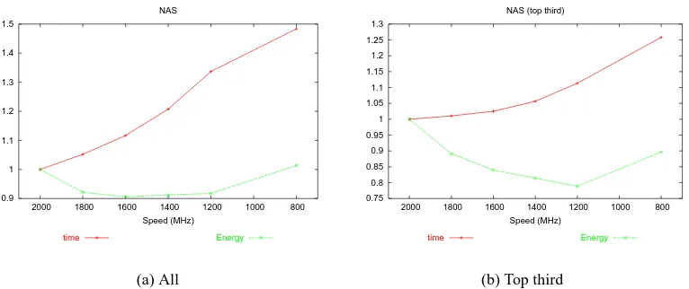
0.9 1 1.1 1.2 1.3 1.4 1.5 800 1000 1200 1400 1600 1800 2000 Speed (MHz) NAS time Energy (a) All 0.75 0.8 0.85 0.9 0.95 1 1.05 1.1 1.15 1.2 1.25 1.3 800 1000 1200 1400 1600 1800 2000 Speed (MHz) NAS (top third)
time Energy
(b) Top third
Figure 3.1: Aggregate plots of NAS set.
3.1
Single-Node Results
Because we studied a large number of programs from three benchmark suites, space
con-straints do not permit the presentation of all the individual results. Therefore, we divide single-node
results into two parts. First, we discuss the overall results. Then, we look at a few representative
applications in detail. Complete individual application results can be found in Appendix A.
Overall Results
All of our tests show that for a given program, using the fastest gear takes the least time.
A slower gear takes more time, and because the CPU is the dominant power consumer, uses less
power. However, in terms of energy, the results vary. If the decrease in power exceeds the increase
in time, a slower gear uses less energy. This is the case all of the programs we tested, where one
of the slower gears results in the least energy consumed. However, it is conceivable that the time
increase could exceed the power decrease, so the fastest gear would also consume the least energy.
Figures 3.1(a), 3.2(a), and 3.3(a) plot the normalized aggregate results for each program
set on AMD 64. (NAS, SPEC INT and SPEC FP) The x-axis plots the gear in terms of frequency
from highest to lowest. There are two lines; the increasing line is elapsed time and the initially
decreasing line is energy consumed. All values are normalized to those of the fastest gear; thus, all
lines begin at 1 on the left-hand side. For the NAS programs, the time and energy diverge from 1
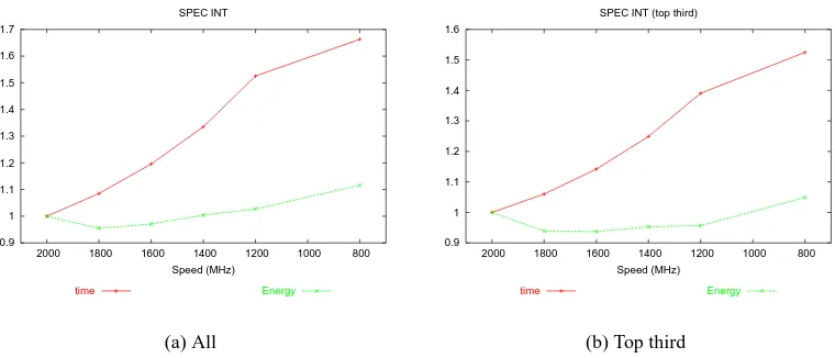
0.9 1 1.1 1.2 1.3 1.4 1.5 1.6 1.7
800 1000 1200 1400 1600 1800 2000
Speed (MHz) SPEC INT
time Energy
(a) All
0.9 1 1.1 1.2 1.3 1.4 1.5 1.6
800 1000 1200 1400 1600 1800 2000
Speed (MHz) SPEC INT (top third)
time Energy
(b) Top third
Figure 3.2: Aggregate plots of SPEC INT set.
at 1600 MHz, the energy used and time taken are 91% and 112% of full, respectively. The SPEC
sets also show an increase in time, but show little decrease in energy. This is because there is a
high variance in the energy-time tradeoff among programs. The SPEC sets contain a few programs
for which there is little energy savings because the fastest gear uses the least energy or close to it.
Overall, the aggregate plots suggest that one needs to be selective about which programs to try to
save energy.
To investigate further, we plot for each set the programs that rank in the top 1/3 of
energy-time tradeoff. Figures 3.1(b), 3.2(b), and 3.3(b) show the results. The NAS subset looks best, with
16% average energy savings for a time delay of less than 3% at 1600 MHz. The SPEC FP subset is
similar, with 12% savings for 7% delay. Finally, the SPEC INT subset provides a 7% savings for a
14% delay.
The slowest two gears do not generally offer energy savings. While the power is
de-creased, the time delay is so great that the energy savings is small if any. However, we notice that
all of the programs have an energy-time tradeoff. The complete results are shown in Appendix A.
The next section evaluates individual programs in detail.
Detailed Results
In this section we analyze six programs in detail: the best and worst in terms of
energy-time tradeoff from each program set. The total system energy consumed at each gear is plotted on
0.9 1 1.1 1.2 1.3 1.4 1.5 1.6 800 1000 1200 1400 1600 1800 2000 Speed (MHz) SPEC FP time Energy (a) All 0.8 0.9 1 1.1 1.2 1.3 1.4 800 1000 1200 1400 1600 1800 2000 Speed (MHz) SPEC FP (top third)
time Energy
(b) Top third
Figure 3.3: Aggregate plots of SPEC FP set.
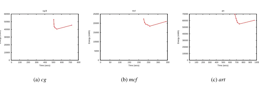
0 10000 20000 30000 40000 50000 60000
0 100 200 300 400 500 600 700 800
Energy (mWh) Time (secs) cg.B (a) cg 0 5000 10000 15000 20000 25000
0 50 100 150 200 250 300 350
Energy (mWh) Time (secs) mcf (b) mcf 0 10000 20000 30000 40000 50000 60000 70000
0 100 200 300 400 500 600 700 800 900 1000
Energy (mWh)
Time (secs) art
(c) art
Figure 3.4: Best energy-time tradeoff in each set.
more energy, and the further right of two points takes more time. Therefore, a near-vertical slope
indicates an energy saving with little time delay between adjacent gears, whereas a horizontal slope
indicates a time penalty and no energy savings.
The programs shown in Figure 3.4 have the best energy-time tradeoff in each sets: NAS
(cg), SPEC INT (mcf ), and SPEC FP (art). In these “vertical” applications, the execution time
advantage of the fastest gear is small. However, the energy penalty for this ultimate performance is
large. Consider for example the cg benchmark, in Figure 3.4(a). Using the third gear (1600 MHz)
yields about a 1% increase in execution time compared to the fastest, while the corresponding
decrease in energy consumption is nearly 20%.
Next, we examine how a vertical energy-time shape occurs. Our results show that
0 5000 10000 15000 20000 25000 30000 35000 40000 45000 50000
0 100 200 300 400 500 600 700 800
Energy (mWh) Time (secs) ep.B (a) ep 0 5000 10000 15000 20000 25000
0 50 100 150 200 250 300 350 400
Energy (mWh) Time (secs) perlbmk (b) perlbmk 0 5000 10000 15000 20000 25000 30000
0 100 200 300 400 500 600
Energy (mWh)
Time (secs) sixtrack
(c) sixtrack
Figure 3.5: Worst energy-time tradeoff in each set.
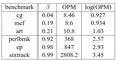
benchmark β OPM log(OPM)
cg 0.04 8.46 0.927
mcf 0.19 8.6 0.934
art 0.21 10.8 1.03
perlbmk 0.92 368 2.57
ep 0.98 847 2.93
sixtrack 0.99 2808.2 3.45
Table 3.2: Predicting CPU boundness.
ever, the number of cycles that an execution takes can change, especially in the vertical applications.
For example, consider the mcf application at the two fastest gears (2000 and 1800 MHz), in which
the performance gain is less than 1%. Using the slower gear with a clock rate that is 90% of the
high-est, the execution has 90% as many cycles (approximately 5.0 to 4.5 trillion). Because the number
of micro-operations does not change, the performance, in micro-operations per cycle (UPC),
in-creases as the frequency dein-creases. The additional cycles in the faster gear do not perform useful
work. This indicates that the CPU is not the performance bottleneck. Below we examine this and,
not surprisingly, determine that memory is the bottleneck.
On the other hand, Figure 3.5 shows the programs that do not exhibit an energy penalty
for the ultimate performance. Instead, in these programs, the fastest gear results in nearly the lowest
energy consumed. We call these “horizontal” programs.
To further quantify the degree of CPU (or memory) boundness, we use an metricβ
intro-duced in [29].β is defined as a ratio between 0 and 1:
β = (T /Tmax−1)
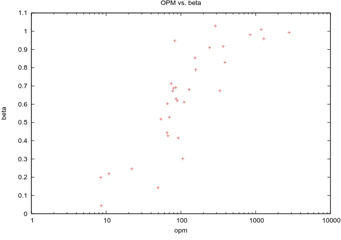
0 0.1 0.2 0.3 0.4 0.5 0.6 0.7 0.8 0.9 1 1.1
1 10 100 1000 10000
beta
opm OPM vs. beta
Figure 3.6: OPM vs.betafor all applications on AMD-64.
whereT andTmax are execution times at a lower frequency and maximum frequency (2000MHz
in this case), respectively, andf andfmax are the corresponding frequencies. Theoretically, if a
program is completely CPU bound, thenT would increase by the amount of increase in cycle time,
T = fmax
f ·Tmax, in which caseβ = 1. On the other hand, if a program is completely independent
of the CPU thenT =Tmaxandβ = 0.
In our tests, the valueβdoes not change significantly as the frequency changes. We found
that on average, for any application, the largest difference in β between running the application
using any two frequencies is around 5%. Column 2 of Table 3.2 showsβ of the six application we
examined, measured between 2000 and 1800 MHz. It is clear that the three “vertical” benchmarks
all have smallβvalues, indicating they are not CPU bound. On the other hand, the three “horizontal”
benchmarks all haveβ close to 1, indicating they are CPU bound. However, one problem withβ
is, while it accurately measures the CPU boundness of an application, we must run the application
twice using different gears to get this measurement. Therefore, we would like to use a metric that
can fairly accurately predictβof an application without such overhead.
The programs we consider in this section do not perform much I/O. Therefore, the
the memory pressure of an application or phase. Similar toβ, OPM stays constant as the frequency
changes. We found that for all the applications we tested, the largest difference in OPM between
running an application using two different gears is about 1%. A large value of OPM means the
program is CPU bound because on average, the program executes more instructions between cache
misses. Table 3.2 shows OPM andβ of the six program we examined. Similar to the trend ofβ, the
three vertical programs, cg, mcf and art, all have small OPM, indicating they are memory bound.
On the other hand, the three horizontal programs all have large values of OPM. One thing to notice
is that in both columns, the values of OPM andβ are sorted. Figure 3.6 shows scatter plot of OPM
vs. βfor all the applications we tested. OPM is plotted on a log scale in this figure because unlike
β, which has a maximum value of 1, the values of OPM are not bounded. In order to better
under-stand the correlation between the two metrics, we uselog(OP M)to relate toβ. We found that the
correlation coefficient is 0.84, indicating a close correlation between OPM andβ.
The advantage of OPM is that unlikeβ, this measurement can be obtained at runtime with
negligible overhead using any gear. OPM is also used to define and sort phases in a single program
in our multi-gear tests, which is described in detail in Chapter 4.
3.2
Multiple-Node Results
The previous section investigated the energy-time tradeoff on a single node. This section
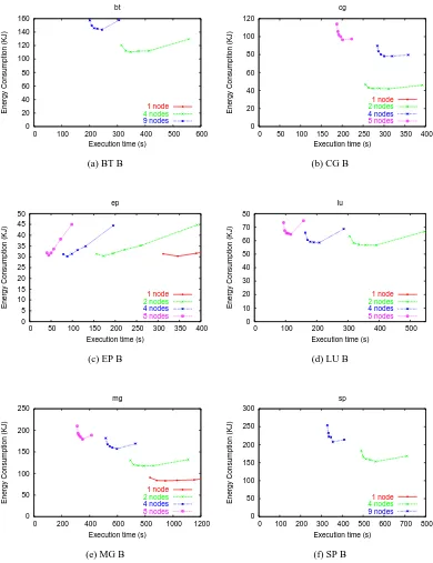
studies the effect of distributed programs. Figure 3.7 shows results from six NAS programs. Each
graph has the same general layout as in Figure 3.4 and Figure 3.5, except that it shows the results
from multiple experiments: 2, 4, and 8 nodes (or 4 and 9 nodes in the case of BT and SP). It also
plots the one-node results from the previous section, but in most cases the data are to the right of
the window of time shown. The energy plotted is cumulative energy of all nodes used.
Before discussing the results, we describe the possible layouts of these graphs. First,
for a fixed number of nodes, the shape of the curve depends on the memory and communication
bottlenecks. This is because in a distributed program, not only might a processor wait for the
memory subsystem, but at times it also might block awaiting a message. In either scenario, the CPU
is not on the critical path, and it is more efficient to execute in a lower energy gear.
Second, consider the possible effects when comparing an experiment with2P nodes
ver-sus one withPnodes. The following possibilities exist. Note that we do not consider the case where
0 20 40 60 80 100 120 140 160
0 100 200 300 400 500 600
Energy Consumption (KJ)
Execution time (s) bt
1 node
4 nodes
9 nodes
(a) BT B
0 20 40 60 80 100 120
0 50 100 150 200 250 300 350 400
Energy Consumption (KJ)
Execution time (s) cg
1 node
2 nodes
4 nodes 8 nodes
(b) CG B
0 5 10 15 20 25 30 35 40 45 50
0 50 100 150 200 250 300 350 400
Energy Consumption (KJ)
Execution time (s) ep
1 node
2 nodes
4 nodes 8 nodes
(c) EP B
0 10 20 30 40 50 60 70 80
0 100 200 300 400 500
Energy Consumption (KJ)
Execution time (s) lu
1 node
2 nodes
4 nodes 8 nodes
(d) LU B
0 50 100 150 200 250
0 200 400 600 800 1000 1200
Energy Consumption (KJ)
Execution time (s) mg
1 node
2 nodes
4 nodes 8 nodes
(e) MG B
0 50 100 150 200 250 300
0 100 200 300 400 500 600 700 800
Energy Consumption (KJ)
Execution time (s) sp
1 node
4 nodes
9 nodes
(f) SP B
1. The curve for 2P nodes can lie completely above and to the left of the curve forP nodes
(more energy, less time). Each point on the2Pnode curve lies above all points on thePnode
curve. This case occurs when the program achieves poor speedup on2Pnodes compared to
P nodes.
2. The point that represents the fastest energy gear for2Pnodes can be to the left, at or below, the
corresponding point on the curve forP nodes. This case occurs when the program achieves
perfect or superlinear speedup on2P nodes compared toP nodes.
3. The curve for2P nodes can lie to the left of the curve forP nodes, but not completely above
or below the fastest gear point forP. This is the most interesting case. While the program
executes faster and consumes more energy in the fastest gear on2P nodes than onP nodes,
there is a lower gear at 2P nodes that has less energy consumption than the fastest gear
point atP nodes. Therefore, it is possible to achieve better execution time and lower energy
consumption by running in a slower gear on2Pnodes than in a faster gear onP nodes. There
is not an energy-time tradeoff between these points because one point dominates the other in
both energy and time. This case occurs case when speedup is good (i.e., not superlinear and
not poor) and there are a significant number of main memory accesses (so that scaling down
the processor has only a slightly detrimental effect).
We describe each of the cases in turn below.
Case 1: Poor Speedup
Figure 3.7 offers several examples of case 1. In particular, this case is illustrated in BT,
SP, and MG from 2 to 4 nodes, and CG from 4 to 8 nodes.
We believe in the future a given supercomputer cluster will be restricted to a certain
amount of power consumption or heat dissipation. If there is a limit for energy/power
consump-tion or heat dissipaconsump-tion, this would be represented as a horizontal line. For programs in this case,
the line will intersect at most one of the curves. The most desirable point would be the leftmost
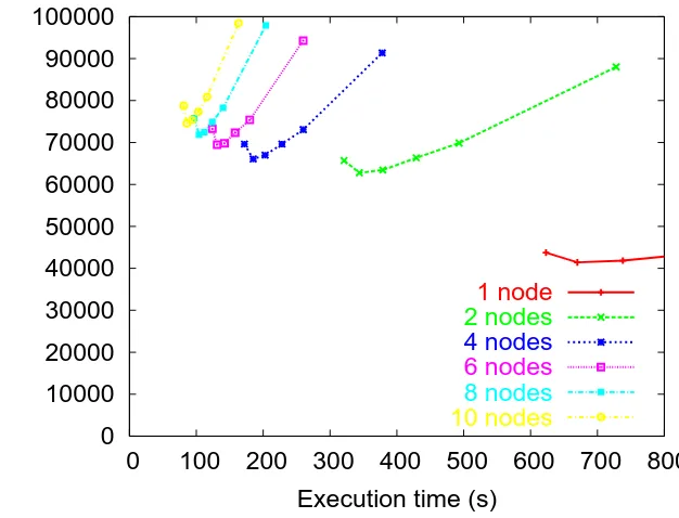
0 10000 20000 30000 40000 50000 60000 70000 80000 90000 100000
0 100 200 300 400 500 600 700 800
Energy consumption (kJ)
Execution time (s)
1 node 2 nodes
4 nodes
6 nodes 8 nodes
10 nodes
Figure 3.8: Energy consumption vs. execution time for Jacobi iteration on 2, 4, 6, 8, and 10 nodes.
Case 2: Superlinear Speedup
Figure 3.7 does not contain an example of superlinear speedup. However, EP, which
gets almost perfect speedup, illustrates this case. Power consumption doubles when the number
of nodes doubles. Because the time is cut in half, the total energy consumed is the same. With
superlinear speedup the energy consumption decreases as nodes are added. When speedup is perfect
or superlinear there is no energy-time tradeoff.
Case 3: Good Speedup
Figure 3.7 shows several examples of this case. First, consider LU at 4 and 8 nodes. Gear
4 on 8 nodes uses approximately the same energy as the fastest gear on 4 nodes, but executes 50%
more quickly. The fastest gear on 8 nodes executes 72% faster than on 4 nodes, but uses 12%
more energy. This case illustrates an additional choice not available in a conventional cluster, which
only supports either the fastest gear option (4 or 8 nodes). So a user must trade off a performance
increase against an energy increase. With a power-scalable cluster, the user can select a slower gear
on 8 nodes, which may offer better performance for the same energy consumption. Thus, a user
0.9 1 1.1 1.2 1.3 1.4 1.5 1.6
0.8 1 1.2 1.4 1.6 1.8 2 2.2 2.4 2.6
Relative energy consumption
Relative execution time
1 node
2 nodes
4 nodes
8 nodes
(a) EP B
0.9 0.95 1 1.05 1.1 1.15 1.2 1.25 1.3
0.8 1 1.2 1.4 1.6 1.8 2 2.2
Relative energy consumption
Relative execution time
1 node
4 nodes
9 nodes
(b) BT B
0.9 0.95 1 1.05 1.1 1.15 1.2
0.8 1 1.2 1.4 1.6 1.8 2
Relative energy consumption
Relative execution time
1 node
2 nodes
4 nodes
8 nodes
(c) MG B
Figure 3.9: Relative energy vs. time.
performance gear. In case 3, the user may be able to get better performance by using more nodes,
with each node executing at a lower energy gear.
Next, Figure 3.8 plots data for a (hand-written) Jacobi iteration application. This
applica-tion is shown because it can run at any number of nodes, unlike the NAS benchmarks. The figure
shows energy-time curves on 5 configurations: 2, 4, 6, 8, and 10 nodes. Because this application
gets good speedup (1.9, 3.6, 5.0, 6.4, and 7.7) each adjacent pair of curves falls in case 3. For
example, executing in second or third gear on 6 nodes results in the program finishing faster and
using less energy than using first gear on 4 nodes.
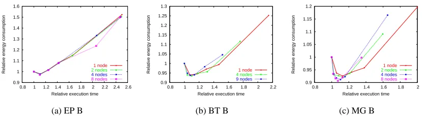
So far we have discussed the results in absolute terms. It is also useful to look at the
relative shapes of the energy-time curves. Figure 3.9 shows the curves for three of the NAS programs
relative to the fastest gear. Therefore, the fastest gear is always plotted at(1,1). These plots are
presented because they represent the three distinct features that have been observed. Figure 3.9(a)
shows EP, in which the shapes essentially overlay each other. This is because EP has almost no
communication. Consequently, the program executes nearly identically on any number of nodes.
The next feature is illustrated by BT in Figure 3.9(b). BT has a large communication
component. While an increase in CPU cycle time increases computation time, it has little effect
on the communication time. Therefore, the increase in execution time due to frequency reduction
is less significant as the computation to communication ratio decreases. This effect is shown in
Figure 3.9(b), as the curve compresses horizontally as the number of nodes increases. For example,
the rightmost (slowest) point decreases from 2.15 to 1.76 to 1.52.
The last feature is illustrated by MG in Figure 3.9(c). This example shows how the curve
becomes more vertical as parallelism increases, indicating that the time penalty decreases. Both
0 10000 20000 30000 40000 50000 60000 70000
0 50 100 150 200 250 300 350 400 450
Energy consumption (kJ)
Execution time (s)
2 nodes 4 nodes
8 nodes
Figure 3.10: Synthetic benchmark with high memory pressure.
munication. The important factor is the relative amounts of computation (executing) and
communi-cation (blocked) time. The gear setting only affects the active portion. Because BT has significant
idle/blocked time (33% and 50% on 4 and 9 nodes, respectively), the gear setting has a small effect
on BT. However, MG has on a much smaller amount of idle time (10%, 13%, and 24% on 2, 4, and
8 nodes, respectively); therefore, the gear setting makes a more pronounced difference.
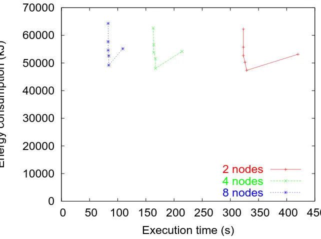
Finally, we present results from a synthetic benchmark. This benchmark models CG in
terms of its cache miss rate, but achieves good speedup (over 7 on 8 nodes). The purpose of this
benchmark is to show the potential of a power-scalable cluster. Figure 3.10 shows the results.
Because the miss rate is high (7%), the execution time penalty for scaling down is low (e.g., 3%
at 1200MHz), and the corresponding energy savings is large (24%). Furthermore, compared to top
Chapter 4
Multiple-Gear Results
This chapter describes the results of using our framework to executing a single program
in multiple gears. (A majority of the results are based on our previous study in [21] and [20]) We
studied seven benchmarks from NAS parallel benchmark suite. All benchmarks are tested using
either 8 or 9 nodes configurations. We divide this chapter into two parts. First, we describe how we
use profiling technique to determine an effective gear for each phase. Then, we analyze the results.
4.1
Profile-Directed Technique
This section describes our profiling technique for determining an effective gear for each
phase. First, it describes detecting and prioritizing phases. Next, it discusses the mechanism that
col-lects performance data which determine the energy-time tradeoff. Finally, it discusses our method
for choosing an assignment of gear to each phase.
Phase Detection This thesis, uses a straightforward programming model, which primarily applies
to iterative and predictable HPC applications. Specifically, it starts by obtaining a trace of the
application in question (run at the fastest gear—highest frequency-voltage setting). From there, it
divides a program into blocks. The term block is motivated by the common compiler term basic
block. In a basic block, all statements must be executed. In a similar way, in a block, all statements
0 20 40 60 80 100 120 140 160
0 200 400 600 800 1000 1200 1400 1600 1800 2000
OPM (operations/miss)
Time (5 ticks/s)
(a) Full trace
0 20 40 60 80 100 120 140 160
200 205 210 215 220 225 230
OPM (operations/miss)
Time (5 ticks/s)
Phase 3 Phase 1 Phase 2 Phase 3 Phase 1 Phase 2 Phase 3
(b) Window from 40–46 seconds.
Figure 4.1: Trace of operations per miss for LU C.
The actual division into blocks is done by examining the trace and using an ad hoc
ap-proach that conforms to the following principles. First, any MPI operation demarcates a block
boundary. Second, a boundary is inserted after any first level inner loops, following the notion that
ends of loop nests are where program characteristics generally change [32]. We do not divide first
level loops any further mainly because it makes block sizes too small to make any measurements,
such as memory pressure. We describe our approach assuming that there is an outermost loop that
consists of a linear list of blocks (i.e., no control flow). While either restriction can be relaxed, doing
so unnecessarily complicates this discussion. Moreover, HPC codes often have one outermost loop,
and MPI calls are generally unconditionally invoked.
From there, we merge blocks into phases. Two adjacent blocks are merged into a phase if
their corresponding memory pressure is within the same threshold used in rule two above. We note
that this is a simple algorithm and may not find all possible phases; our focus is not on developing
new phase detection techniques. Our plan in the future is to use the significant work on phase
detection that has previously been done—both by compiler [32, 50, 41] and dynamically [30, 11].
As described in Chapter 3, we introduce the metric operations per miss (OPM) as a
mea-sure of the memory presmea-sure of an application or phase. We have found OPM to be effective in
determining phase boundaries. For example, Figure 4.1 gives an example of how OPM varies in the
LU C benchmark on one of 8 nodes. The right-hand figure shows a window of 6 seconds. Here,
OPM clearly partitions the code into three distinct phases. These phases were determined by hand,
130 135 140 145 150 155 160 165
900 1100 1300 1500 1700 0.95 1 1.05 1.1 1.15 1.2 1.25 1 1.2 1.4 1.6 1.8 2
Energy consumption (kJ)
Execution time (s)
(a) BT B
58 60 62 64 66 68 70 72
500 550 600 650 700 0.825 0.85 0.875 0.9 0.925 0.95 0.975 1 1 1.05 1.1 1.15 1.2 1.25 1.3 1.35 1.4 1.45
Energy consumption (kJ)
Execution time (s)
(b) CG B
45 50 55 60 65
350 400 450 500 550 600 650 700 750 1 1.1 1.2 1.3 1.4 1.5 1 1.25 1.5 1.75 2 2.25 2.5
Energy consumption (kJ)
Execution time (s)
(c) EP B
Figure 4.2: Energy consumption vs. execution time for three NAS benchmarks on a single AMD machine.
Phases Prioritization Our method for assigning gears to phases requires ordering the phases such
that the most likely phases to benefit from running at a lower gear are identified. This allows our
algorithm to run in linear time, yet still find the desired solution. Thus, our approach requires
distinguishing a phase that has a good energy-time tradeoff from one that does not. That is, we
must estimate the effect executing a phase in a slower gear will have on the energy consumption
and execution time of the block. The key here again is OPM (introduced above), which estimates
the phases that have a good energy-time tradeoff.
Figure 4.2 shows the results of executing 3 NAS programs on a single Athlon-64
pro-cessor. EP is CPU bound and therefore has a large time penalty and little or no energy savings at
reduced gears. On the other hand, CG is memory bound, so the time penalty is almost nothing. BT
is a more typical application that sits between the extremes of EP and CG.
Data Collection The first step gathers profile data during an execution of the program. This
implementation uses our MPI-jack tool, which is an interface that exploits PMPI [49], the profiling
layer of MPI. MPI-jack enables a user transparently to intercept (hijack) any MPI call. A user can
execute arbitrary code before and/or after an intercepted call. These are called pre and post hooks.
In this work, we use MPI-jack to shift gears in post hooks.
The first step involves sampling an application, producing profile or trace data. An
appli-cation is sampled at every phase boundary. This is done entirely through MPI-jack; in the case of
MPI calls, it is trivial to add the sampling code. When it is necessary to insert a phase boundary at
the end of a loop nest (i.e., not at the end of an MPI call), we simply insert a pseudo MPI call; this
/*Gis ann-dimensional vector of gear selections, one for each phase.*/ setGk= 0,∀k|0≤k < n /*The top gear is 0; slowest gear isn−1*/
givenT /*Tuple (energy,time) for currentG(initially the baseline)*/
given≺ /*A user-defined relationship that defines total order ofT */
/*Invoke the function to start method that produces final solution,Gf */
Gf ←evaluate(program, G,0, n, T)
defineevaluate(program, G, i, n, T)
ifi≥norGi≥gslowestthen returnGfi Gi←Gi+ 1
execute program using solutionG
measure energy and time forG, store tuple inT0
ifT0 ≺T then /*T0is not better thanT */
Gi←Gi−1
G= evaluate(program, G, i+ 1, n, T)
else /*T0is better thanT*/
G= evaluate(program, G, i, n, T0)
fi
returnG
end
Figure 4.3: Heuristic for searching solution space.
The information we collect includes the type of call and location (program counter). It
shows status (gear, time, etc.) and metrics (µops and L2 cache misses, so OPM can be computed).
Note that our inclusion of the program counter bears some resemblance to existing program counter
based techniques [22], though that work is aimed solely at saving energy in the disk.
Energy-Time Tradeoff Our analysis (see below) requires energy consumption data; however, we
have found that energy cannot be measured accurately if the period of measurement is too fine
grain.1 For this thesis, as the benchmark programs complete relatively quickly, we measure energy
at the coarsest grain possible—the complete run of a program. (For longer running programs we
can terminate a test run after a fixed number of iterations or phases.)
Determining which of two solutions is “better” depends on how a user wants to trade off
energy savings and time delay. This work does not impose an evaluation. Rather, it leaves it to the
1
user or cluster administrator to select the metric. It could be energy-delay or energy-delay squared,
the latter proposed in [38, 23] has been adopted by Cameron et al. [5] for use in power-aware,
high-performance computing.
Methodology Given a program partitioned into phases, we proceed to our method for determining
an effective assignment of gears to phases. If there arenphases and ggears, than the number of
possible solutions (phase-gear assignments) for the program is gn. In general, this is too large
to explore by brute force. Therefore, the second part of our method is a heuristic (described in
Figure 4.3) that we use to find the “best” solution. The heuristic finds the “best” gear in a phase,
then moves on to the next phase. Once it moves on to another phase, the gear for the preceding
phase has been determined.
Initially, the solutionG(a vector of gears) is set to the baseline value—all zeroes. (Gear 0
is the baseline gear, which is also the fastest. The gear number indicates the number of steps slower
than the baseline) The recursive function is invoked on the 0th phase. It executes the program
using the next slower gear in this phase (all other phases are as before). If the energy-time tradeoff
(defined by a user relation, see below) of this new solution is better than the current solution, it is
accepted. The algorithm recursively tries the next lower gear on this phase. The gear is determined
when the new tradeoff is worse than the current or when there are no slower gears. After fixing the
gear, it moves on to the next phase. This heuristic has running time at mostn·g.
After each program execution, the energy and time are measured and compared via the
user-defined relationship. For our tests, we use a simple and intuitive evaluation of the tradeoff based
on the slope of the line between two solutions. The slope is defined as the ratio of energy savings
to time delay: ETi−i−ETjj, for two solutions iandj. Thus a slope of -1 (i.e., 45◦ below the horizon)
means savings and delay are equally weighted. A user-defined limit of 0 means minimize energy,
and−∞means minimize time. We consider a new solution with a larger slope (in magnitude) than
the user-defined limit to be better. We do not advocate this metric instead of the others. We use it
because it is reasonable and it is easy to visualize.
Now we show an example of how our methodology works by studying BT class C in
depth. In the graph shown in Figure 4.4, the baseline is the leftmost (fastest) point, where the top
gear, 2000MHz, is used for the entire program. (As before, the higher of two points uses more
energy, and the further right of two points takes more time.) For all other points, at least one phase
is executed in a lower gear. Each point is labeled as a tuple, where theithentry represents the gear
57000 58000 59000 60000 61000 62000 63000 64000 65000
480 490 500 510 520 530 540 550 560 570
Energy (J)
Time (s) 00
11 01
02
03
04
12 13
22 23 14
10
hull
-5/+5
Figure 4.4: Energy-time plot of many BT runs.
have a different number of phases.) For convenience, we refer to a tuple of phase-gear assignments
as a solution.
Our analysis of the operations per miss (OPM) identified two phases in BT. The baseline
solution is labeled “00,” meaning both phases are run in gear 0. In the figure we have drawn a line
connecting 5 points that are “good” choices under a simple slope-based energy-time metric. The
line forms a convex hull that is left of and below all other solutions. Any solution “inside” the hull
is not a “good” choice according to this metric, although there may exist solutions inside the hull
that are good under a different metric.
Recall that the goal of our profiling algorithm is to do “better” than the baseline. As our
chosen metric is the slope between two solutions,L, our algorithm will select a unique point on the
hull. This is illustrated in Table 4.1, which shows five different cases regarding BT, which select the
five solutions on the convex hull.
In the first case (Table 4.1(a)), L is steep (large negative number). Such a value favors
time delay over energy savings. In this case and all others, the algorithm adjusts gears from right
to left across solutions or tuples. Thus, the first test is solution01. The steps of the algorithm are
Solutions Slope < L?
1 00→01 -11.7 false
2 00→10 -1.39 false
00is best
(a) Case 1:−12> L.
Solutions Slope < L?
1 00→01 -11.7 true
2 01→02 -1.78 false
3 01→11 -1.01 false
01is best
(b) Case 2:−1.78> L >−12.
Solutions Slope < L?
1 00→01 -11.7 true
2 01→02 -1.78 true
3 02→03 -1.19 false
4 02→12 -1.44 false
02is best
(c) Case 3:−1.44>L>−1.78.
Solutions Slope < L?
1 00→01 -11.7 true
2 01→02 -1.78 true
3 02→03 -1.19 false
4 02→12 -1.44 true
5 12→22 -0.25 false
12is best
(d) Case 4:0> L >−1.44.
Solutions Slope < L?
1 00→01 -11.7 true
2 01→02 -1.78 true
3 02→03 -1.19 true
4 03→04 0.17 false
5 03→13 -1.20 true
6 13→23 0.97 false
13is best
(e) Case 5:L= 0.
indicates the direction of the slope. Of these two solutions, the energy and time of the one on the
left is known, so only one run of the program is necessary to complete this step. The third column
shows the slope, and the fourth column indicates whether is it less than the user-defined limit. In the
first step, the slope from00to01is greater thanL(not as steep); therefore, it is rejected. We back
up to the previous solution (00) and try the next phase to the left (which in this case happens to be
the leftmost phase). In step 2, solution10is rejected. Thus, the algorithm selects00, the baseline,
whenLis sufficiently steep.
Table 4.1(b) shows the steps in the second case. In this case, 01 is accepted but02 is
rejected. The algorithm fixes the second phase at gear 1 and then determines the gear for the first
phase, ultimately selecting 01. The next case (Table 4.1(c)) is similar; the slope limit is slightly
larger (less steep), which results in acceptance of02, followed by the rejection of03and12.
Table 4.1(d) shows the steps in case 4. In this case, the second phase is fixed at gear 2.
The solution for12is considered better than02, so the algorithm accepts it and tries22, which is
rejected.
The last case is shown in Table 4.1(e). This case temporarily selects solution03, which
is not on the convex hull, before eventually selecting13. The solution03is interesting, because
the algorithm and evaluation metric we describe here will never select it. This is because our slope
metric only picks solutions that are on the convex hull. However, it is a reasonable solution in that
there does not exist a solution that is better than it in both time and energy (i.e., “dominates” it). So,
it easily can be argued that03is better than02. For BT, solutions03and11fall into this category
and therefore may be selected by a different evaluation metric. However, the other solutions (04,
10,14,22, and23) will never be selected by any metric, because each is dominated in both energy
and time by at least one other solution.
4.2
Analysis of Results
Figure 4.5 shows results from the other six NAS programs that we executed. Because
each graph has different x and y ranges, we plot a normalizing line that shows a 5% decrease in
energy and a 5% increase in time. It is important to consider both the direction and magnitude of
this line. Overall, the behavior of the applications varies widely. Each program falls into one three
groups based on its benefit from using a reduced gear. In each figure, we show the convex hull along
39500 40000 40500 41000 41500 42000 42500 43000 43500 44000 44500 45000
390 400 410 420 430 440 450 460 470 480 490 500
Energy (J) Time (s) 0 1 2 3 4 5 hull -5/+5
(a) CG C
41000 41500 42000 42500 43000 43500 44000 44500 45000 45500
230 240 250 260 270 280 290 300
Energy (J) Time (s) 0 1 2 hull -5/+5
(b) EP C
11000 11500 12000 12500 13000 13500
129 130 131 132 133 134 135 136
Energy (J) Time (s) 00 11 22 01 02 13 12 03 04
05 15
hull -5/+5
(c) IS C
58000 59000 60000 61000 62000 63000 64000
440 450 460 470 480 490 500 510
Energy (J) Time (s) 000 001 011 002 021 111 031 121 112 221
321 222 211 223 113 020 012 311 hull -5/+5
(d) LU C
32500 33000 33500 34000 34500 35000 35500 36000 36500 37000 37500
310 320 330 340 350 360 370 380 390 400 410
Energy (J)
Time (s) 00
11 01
02 03 04 05 12 32 42 14 33 44 hull -5/+5
(e) MG C
78000 80000 82000 84000 86000 88000 90000 92000 94000 96000 98000 100000
740 760 780 800 820 840 860 880 900
Energy (J) Time (s) 00 11 01 02 03 04
22 13 23 33 43 10 hull -5/+5
(f) SP C
Multiple Gear Benefit Applications in this group show significant benefit from a multiple-gear
solution. This is the case whenever severalij solutions, wherei6=j, fall on the convex hull. Four
of the seven NAS programs have this characteristic: MG, BT, LU, and IS. For example, in
multiple-gear solution 32, MG saves 11% energy with a 4% time penalty over the baseline. On the other
hand, the single-gear solution33 saves 10% energy with a 7% time delay. BT using solution12
saves 10% energy with a 5% time penalty over the baseline. This compares favorably to single gear
solutions11and22, which yield energy-time tradeoffs of -6%/4% and -8%/17%, respectively.
In the case of LU, there are three phases, as shown above in Figure 4.1. This program is
the only one for which we identified more than two phases. This plot has more points than any other
plot, yet 70 more points are needed to exhaustively search just the top three gears (0 thru 2).
IS is an extreme case, where the first phase is CPU bound and the second phase is both
memory and disk bound. Therefore, a single-gear solution is bound to be poor, as it is necessarily
a compromise solution. Regardless of the desire of the user, single-gear solutions (other than the
baseline) are dominated by points on the hull. The 05solution in IS saves 16% energy over the
baseline (00) at a cost of a 1% time increase. Compared instead to 22, this solution saves 9%
energy and executes 1% faster.
Single Gear Benefit Applications in this group show significant benefit from using a single lower
gear, but no significant benefit from multiple-gear solutions. CG and SP fall into this category. In
CG, only one phase was detected. The application is highly memory bound: its is OPM an order of
magnitude smaller than any other. Moreover, all blocks in the loop have comparable OPM. In SP,
while we found two phases, there is almost no benefit to running phases in different gear. Although
23is on the convex hull, it barely makes it.
Besides the reason given above, there is a second reason that a single gear benefit is all
that can be achieved. Conceptually, an application can fall into the single gear category because
the phases are too fine-grain (possibly because there are too many) and the cost of switching gears
outweighs the benefit. However, this was not the case in any of the NAS programs.
No Benefit Only EP falls into this category. Simply put, EP has only one phase, no communication
(except once at the end of the program), and is CPU bound. Therefore, a reduction in the gear results