ABSTRACT
WEINFURTHER, KYLE JAMES. Designing an Optically Segmented Single-Volume Neutron Scatter Camera Using Simulation and Experimental Validation. (Under the direction of John Mattingly).
© Copyright 2019 by Kyle James Weinfurther
Designing an Optically Segmented Single-Volume Neutron Scatter Camera Using Simulation and Experimental Validation
by
Kyle James Weinfurther
A dissertation submitted to the Graduate Faculty of North Carolina State University
in partial fulfillment of the requirements for the Degree of
Doctor of Philosophy
Nuclear Engineering
Raleigh, North Carolina 2019
APPROVED BY:
Joseph Doster David Lalush
Erik Brubaker John Mattingly
BIOGRAPHY
TABLE OF CONTENTS
LIST OF TABLES . . . v
LIST OF FIGURES . . . vi
Chapter 1 Introduction . . . 1
1.1 Neutron Scatter Imager Functionality . . . 2
1.1.1 Theory . . . 2
1.2 Optically Segmented Pillar Based Scatter Imager . . . 4
1.2.1 SVSC-PiPS Detection Efficiency . . . 6
1.3 Novel Contributions . . . 7
1.4 Background . . . 9
1.4.1 Prior Work . . . 9
1.4.2 Organic Scintillators . . . 13
1.4.3 Photodetectors . . . 15
1.4.4 Scintillation Light Transport . . . 17
1.5 Dissertation Organization . . . 19
Chapter 2 Nominal and Observed Response Construction Methods . . . 20
2.1 Nominal Responses . . . 21
2.1.1 Scintillator Time Response Models . . . 22
2.1.2 Optical Photon Transport Simulations . . . 24
2.1.3 Photodetector Impulse Response and Transit Time Spread . . . 34
2.1.4 Constructing Nominal Responses . . . 36
2.2 Observed Responses . . . 38
Chapter 3 Scintillation Position, Scintillation Time, and Proton Recoil En-ergy Estimation . . . 41
3.1 Alternative Methods to Estimate Scintillation Position . . . 43
3.2 Analysis Method. . . 46
3.2.1 Cost Function . . . 47
3.2.2 Initial Guess . . . 48
3.3 Estimation of Scintillation Position, Proton Recoil Energy, and Scin-tillation Time using MLE . . . 48
3.3.1 Scintillation Position Estimate Precision . . . 50
3.3.2 Proton Recoil Energy Estimate Precision . . . 50
3.3.3 Scintillation Time Estimate Precision . . . 52
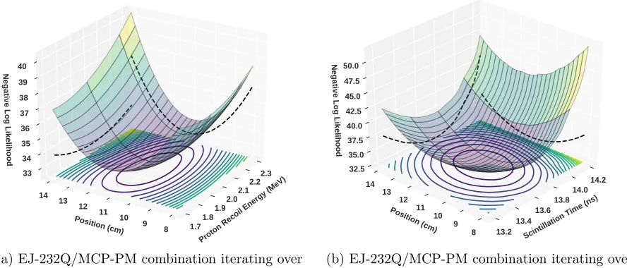
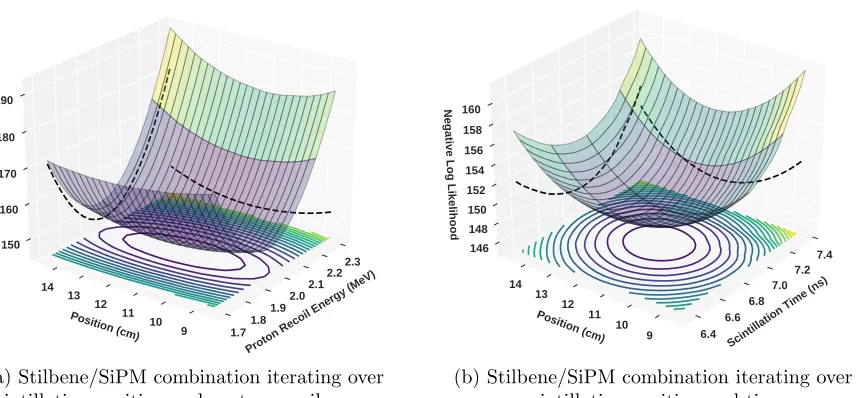
3.3.4 Cost Function Surface Analysis . . . 53
3.3.5 Precision of Position Dependent Reconstruction . . . 56
3.3.6 Reconstruction Results . . . 57
3.4 Position, Energy, and Time Reconstruction Conclusions . . . 61
4.1 Microchannel Plate Single Photoelectron Response Characterization . 64
4.1.1 Experiment Setup . . . 65
4.1.2 Pixel Centering . . . 65
4.1.3 MCP-PM Characterization . . . 67
4.1.4 Characterization Results . . . 68
4.1.5 Characterization Issues . . . 71
4.1.6 MCP Characterization Conclusions. . . 72
4.2 EJ-204 Pillar Experiment . . . 73
4.2.1 Experimental Setup. . . 73
4.2.2 Calibration . . . 75
4.2.3 Pillar Characterization . . . 75
4.2.4 Experiment Results . . . 79
4.2.5 Discrepancies Between Simulation and Experiment . . . 80
4.2.6 Experiment Conclusions . . . 83
Chapter 5 Source Localization . . . 84
5.0.1 MCNPX-PoliMi Simulations . . . 85
5.1 Back-Projected Images . . . 85
5.1.1 Distance Between Neutron Double Scatters . . . 89
5.1.2 Proton Recoils in Neighboring Pillars . . . 90
5.1.3 Removal of Inaccurate Pointing Vectors . . . 92
5.2 MLE Images . . . 100
5.3 Source Localization Conclusions . . . 103
Chapter 6 Conclusions and Future Work . . . .105
6.1 Conclusions . . . 105
6.2 Future Work . . . 107
6.2.1 SVSC-PiPS Readout . . . 107
6.2.2 Neutron and Gamma-ray Discrimination . . . 107
6.2.3 Geant4 Light Transport . . . 108
BIBLIOGRAPHY . . . .109
APPENDICES . . . .115
Appendix A RMS Error Reduction from the Light Output Equations . .116
LIST OF TABLES
Table 2.1 Modeled scintillator properties . . . 23 Table 2.2 Modeled photodetector properties . . . 35 Table 3.1 RMS errors for position, time, and proton recoil energy for three
scintilla-tor/photodetector combinations . . . 50 Table 5.1 Number of cones back-projected for each image when estimating detector
resolution . . . 96 Table 5.2 Fraction of simulated events using MCNPX-PoliMi that produce usable and
unusable pointing vectors . . . 97 Table 5.3 Possible use scenarios for removing incorrect pointing vectors with three proton
recoils . . . 100 Table B.1 10 cm length pillars simulation results, 1 MeV proton recoil energy using 1
mm air gap and ESR lining the housing walls . . . 124 Table B.2 20 cm length pillars simulation results, 1 MeV proton recoil energy using 1
mm air gap and ESR lining the housing walls . . . 125 Table B.3 10 cm length pillars simulation results, 2 MeV proton recoil energy using 1
mm air gap and ESR lining the housing walls . . . 126 Table B.4 20 cm length pillars simulation results, 2 MeV proton recoil energy using 1
mm air gap and ESR lining the housing walls . . . 127 Table B.5 20 cm length pillars simulation results, 1 MeV proton recoil energy with the
ESR film greased directly onto the scintillator . . . 128 Table B.6 20 cm length pillars simulation results, 2 MeV proton recoil energy with the
LIST OF FIGURES
Figure 1.1 Neutron scatter imager operational principles . . . 2
Figure 1.2 Five cone back-projected image . . . 4
Figure 1.3 Compact neutron scatter camera made of optically segmented pillars of scintillator and reflective channels. . . 6
Figure 1.4 Event detection threshold comparison for a dual plane scatter camera and an SVSC-PiPS . . . 7
Figure 1.5 Sandia National Lab neutron scatter camera . . . 12
Figure 1.6 Pulse shape effects from different charged particles . . . 13
Figure 1.7 Conversion from recoil energy to light produced in scintillator . . . 14
Figure 1.8 MA-PMT and MCP-PM charge multiplication mechanisms . . . 16
Figure 1.9 Specular and diffuse reflection angles . . . 18
Figure 2.1 Scintillator time responses . . . 23
Figure 2.2 Scintillator emission spectra . . . 24
Figure 2.3 Cross section of pillar geometry in Geant4 . . . 25
Figure 2.4 Light collection efficiency using various reflectors . . . 27
Figure 2.5 Reflector effect on collected photon wavelength spectrum . . . 28
Figure 2.6 Optical light simulation emission angles . . . 30
Figure 2.7 Optical photon transport results as a function of time of arrival . . . 30
Figure 2.8 Optical photon transport results as a function of emission angle . . . 31
Figure 2.9 Pillar impulse responses . . . 32
Figure 2.10 Simulated light collection efficiency for 10 cm, 20 cm, and 50 cm pillars . . . 33
Figure 2.11 Photon arrival time histogram for a 20 cm EJ-204 pillar with different widths 34 Figure 2.12 Photodetector impulse responses . . . 35
Figure 2.13 Transit time spread model (RT T S(t)) . . . 37
Figure 2.14 Nominal responses from a 1 cm x 1 cm x 20 cm scintillator pillar with an air gap and ESR film . . . 37
Figure 2.15 Simulated observed waveform production method . . . 40
Figure 3.1 Scintillation position estimates using relative light intensity and time of arrival 45 Figure 3.2 Observed and best fit waveforms . . . 49
Figure 3.3 Error in position reconstruction for 10,000 events uniformly distributed throughout the pillar for 2 MeV proton recoil energy. . . 51
Figure 3.4 Error in proton recoil energy reconstruction . . . 51
Figure 3.5 Scintillation time RMS errors for three scintillator/photodetector combinations 52 Figure 3.6 3-D negative log likelihood surfaces for EJ-204/MA-PMT . . . 54
Figure 3.7 3-D negative log likelihood surfaces for EJ-232Q/MCP-PM . . . 55
Figure 3.8 3-D negative log likelihood surfaces for stilbene/SiPM . . . 56
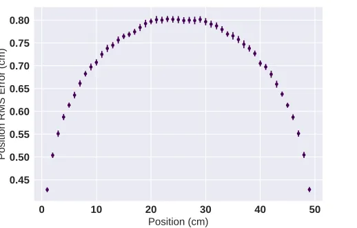
Figure 3.9 Position RMS errors across the length of the pillar for a 50 cm pillar . . . 57
Figure 3.10 Reconstructed position and proton recoil energy RMS errors . . . 59
Figure 3.11 Reconstructed position and scintillation time RMS errors . . . 60
Figure 4.1 Planacon XP85012 schematics . . . 64
Figure 4.2 MCP-PM characterization experimental setup . . . 66
Figure 4.3 MCP-PM pixel centering measurement . . . 66
Figure 4.4 Single photoelectron pulse height distribution . . . 67
Figure 4.5 MCP-PM pixel occupancy . . . 69
Figure 4.6 MCP-PM mean single PE area . . . 70
Figure 4.7 MCP-PM single PE area standard deviation . . . 70
Figure 4.8 MCP-PM average single PE waveforms . . . 71
Figure 4.9 MCP-PM typical cross talk waveform . . . 72
Figure 4.10 EJ-204 pillar experimental setup . . . 74
Figure 4.11 Light intensity characterization results as a function of position for the EJ-204 pillar. . . 76
Figure 4.12 EJ-204 pillar time of arrival characterization results . . . 77
Figure 4.13 EJ-204 pillar average waveforms . . . 78
Figure 4.14 EJ-204 pillar scintillation position estimate results . . . 79
Figure 4.15 Comparison of simulated and experimental expected waveform dilation . . . 81
Figure 5.1 Back-projected image results . . . 87
Figure 5.2 Normalized 1-D profiles of a back-projected image . . . 88
Figure 5.3 Distance traveled by neutrons after first proton recoil . . . 89
Figure 5.4 Probability of neutron double scatter in the same pillar with neutrons directed parallel to length of pillar . . . 90
Figure 5.5 Probability of neutron double scatter in the same pillar with neutrons directed orthogonal to length of pillar . . . 91
Figure 5.6 Probability to double scatter in same pillar based on pillar size . . . 92
Figure 5.7 Double scatter location proximity effect on pointing vector . . . 93
Figure 5.8 Back-projected images excluding neighboring pillars . . . 94
Figure 5.9 Back-projected image resolution as a function of the number of back-projection cones . . . 95
Figure 5.10 SVSC-PiPS FWHM contour lines for back-projected images using thresholds of 0.5, 1.0 and 1.5 MeV. . . 96
Figure 5.11 Neutron scatter profiles for events with greater than one proton recoil . . . . 98
Figure 5.12 MLE image 2-D profile over azimuth angle as a function of MLE iterations . 101 Figure 5.13 Images produced after 15 MLE iterations . . . 102
Figure 5.14 Back-projected image profile from MLE iterations . . . 103
Figure A.1 EJ-309 light output function and its inverse . . . 120
CHAPTER
1
INTRODUCTION
The localization of neutron emitting sources can be accomplished using neutron scatter imagers. The purpose of a neutron scatter imager is to point in the direction of a neutron emitting source. Neutron scatter imagers use the kinematics of elastic neutron scattering by hydrogen to estimate the direction of a neutron source.
1.1
Neutron Scatter Imager Functionality
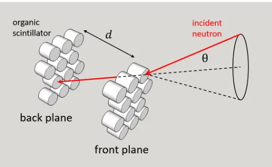
Neutron scatter imagers estimate incident neutron direction using the kinematics of neutron scattering off hydrogen-1 in an organic scintillator. A neutron must scatter twice within the active volume of the detector to estimate incident neutron direction. The location of both scatters, the time between scatters, and the energy deposited in the first scatter are used to identify a cone of possible incident neutron directions whose axis is aligned with the vector connecting the two scatters. This vector is known as the “pointing vector”. Figure 1.1 illustrates this method using a dual plane scatter imager.
Figure 1.1 Neutron scatter imager operational principles. Incident neutron cone angles are estimated using the time-of-flight (TOF) of the neutron between the two planes and the scintillation brightness from neutron elastic scatter in the front plane
1.1.1 Theory
Neutrons transfer some or all of their energy to the organic scintillator during elastic scatter [33]. The amount of energy transferred is dependent upon recoil nucleus mass and the angle of scatter given by
En0 = (1 +α) + (1
−α) cosθCM
where α =
A−1 A+ 1
2
,A is the atomic mass of the target nucleus, En is the incident energy of the neutron, En0 is the energy of the neutron after elastic scatter, and θCM is the scatter
angle in the center-of-mass (CM) coordinate frame. Scattering by light nuclei is isotropic in the center-of-mass coordinate frame, and neutrons transfer all of their energy to a proton (A= 1) in a head-on collision when θCM = 180◦. The center-of-mass scattering angle is related to angle in the lab frame by
tanθL= 1 sinθCM A + cosθCM
(1.2)
where θL is the lab frame scattering angle [33]. We can simplify Equation 1.1 and Equation 1.2 to calculate the scattered neutron angle in the lab frame. For hydrogen-1 scatter, the energy Ep of the recoil nucleus (a proton) is given by
Ep =En−En0 (1.3)
where the energy of the proton is the energy difference of the incoming and outgoing neutron. Again, for hydrogen-1 scatter, (A= 1) such that α= 0. Combining Equations 1.1 and 1.2 yields
Ep =Ensin2θL (1.4)
whereθL is the angle between the incident neutron and the scattered neutron directions in the lab frame. We cannot directly measure the incident energy of the neutron; however, Ep can be estimated from the brightness of the first interaction, andEn0 can be estimated from the
time-of-flight between the two scatters. The scattered neutron energyEn0 is estimated using
En0 = 1 2mnv
2 = 1
2mn
d ∆t
2
(1.5)
A second neutron scatter must occur, otherwise scattered neutron energy cannot be estimated and cone back-projection is impossible. We can simplify Equation 1.4 using Equation 1.3 to eliminate En resulting in
θL=tan−1
s
Ep En0
!
(1.6)
where the opening angle of the back-projected cone is in terms of the proton recoil and scattered neutron energy. Back-projected cones overlap to produce a hot-spot in the image as illustrated in Figure 1.2. The hot-spot displayed in the center of the figure is the most likely direction of a neutron source.
Figure 1.2 Back-projected image from five cones. The hot-spot in the center of the figure is the most likely direction of a neutron source.
1.2
Optically Segmented Pillar Based Scatter Imager
the camera. After a neutron elastically scatters in the front plane, there is a small solid angle for the neutron to travel in the direction of the back plane. Most neutrons will only single scatter in the front plane and not interact with the back plane, which reduces the overall efficiency of the imager.
Pixelated photodetectors with small form factors and large active areas have recently become commercially available. Millimeter scale position resolution is possible with current pixelated photodetectors. Instead of using two planes for imaging, imagers can be reduced to a single active volume using these advancements. The position (x, y, z), intensity (L), and time (t) of both elastic scatters are required when a neutron interacts twice within the volume to perform cone back-projection.
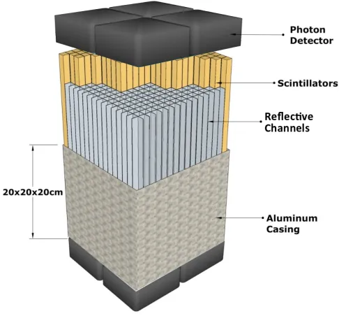
We propose a high efficiency imager design to localize neutron emitting material. A depiction of this imager, a single volume scatter camera made of pillars of plastic scintillator (SVSC-PiPS) is shown in Figure 1.3 [76]. The instrument design uses a contiguous volume of organic scintillator that is subdivided into optically isolated pillars. Each scintillator pillar is surrounded by a small air gap; this air gap allows scintillation light to undergo total internal reflection (TIR) to increase light collection efficiency. Each channel is surrounded by a reflector to redirect photons escaping back into the pillar. Orthogonal to each pillar and attached to opposing ends are photodetectors. The photodetectors enable two waveforms to be recorded for each neutron elastic scatter. The device consists of a scintillating volume on the order of 10 liters. The major advantage of using a single active volume is the significantly higher probability of a second scatter within the device. After the first elastic scatter, the neutron is enveloped in the detector; any direction the neutron travels, a second elastic scatter is likely to occur.
Figure 1.3 Compact neutron scatter camera made of optically segmented pillars of scintillator and reflective channels.
1.2.1 SVSC-PiPS Detection Efficiency
We compared the efficiency of a dual plane imager and an SVSC device using the simulation tool MCNPX-PoliMi [55]. The dual plane imager was modeled after a two plane neutron scatter camera (NSC) built at Sandia National Laboratories (described in more detail later in this chapter). MCNPX-PoliMi is a Monte Carlo particle transport code that records state variables (e.g. position, direction, incident energy, and energy deposited) for particles that interact in user-specified detector cells. We calculated the efficiency of the two devices as a function of the proton recoil energy threshold shown in Figure 1.4. The simulation consisted of a pencil beam of fission spectrum neutrons aimed at the center of both devices. We simulated an NSC with 40 cm between the two planes, which is typical. For both simulations, we only analyzed events where the first two interactions were off hydrogen-1.
0.5 1.0 1.5 2.0 2.5 3.0 Scatter Threshold (MeV)
10
510
410
310
210
1Double Scatter Frequency
SVSCPiPS NSC
Figure 1.4 Event detection threshold comparison for a dual plane scatter camera and SVSC-PiPS for a pencil beam of Cf-252 fission spectrum neutrons aimed at the center of the respective device.
the first two hydrogen-1 scatters could not occur in the same pillar; for the dual plane imager, a neutron must scatter on hydrogen-1 for both the first scatter in the front plane and the second scatter in the back plane.
Figure 1.4 shows that the single volume design has significantly higher efficiency by about an order of magnitude. At a 200 keV threshold for both neutron scatters, the dual plane scatter camera has about 1% efficiency. Using a contiguous volume of scintillator results in an order of magnitude efficiency increase. Even though the SVSC-PiPS has approximately one quarter the active volume of the dual plane imager, its efficiency is an order of magnitude greater because the double scatter probability is higher for a contiguous volume than a dual plane design.
1.3
Novel Contributions
Recent advancements in photodetector technology have enabled the development of a compact neutron scatter camera. The main advantage of a single volume scatter camera is an order of magnitude increase in efficiency relative to dual plane designs.
photodetectors attached to (at least) two opposing sides of the block [9]. When the scintillator block is contiguous, all photodetector pixels must be digitized to estimate position (x, y, z), scintillation time (t), and intensity (L) which requires large data throughput. Additionally, scintillation light from the first interaction can overlap in time with light from the second interaction. This creates difficulty when assigning scintillation photons to individual interactions. In contrast, the optically segmented design presented in this dissertation confines scintillation light to a single pillar using reflectors lining the housing walls. Light is confined to a single pillar, so its collection is unique to each interaction which enables independent analysis of individual elastic scatters; therefore, parameter estimation is decreased from five parameters (x, y, z, t , L) to three parameters (z, t, L). (x, y) is identified by the pillar collecting light. This design enables the estimation of scintillation position, scintillation timing, and intensity from the amplitude and relative timing of the observed photodetector signals compared to nominal (expected) responses using maximum likelihood estimation. For a 1 cm x 1 cm x 20 cm EJ-204 pillar using an MA-PMT photodetector and greater than 1 MeV proton recoil energy, we estimated:
• Less than 1 cm RMS error for scintillation position
• Less than 50 keV RMS error for proton recoil energy
• Less than 100 ps RMS error for scintillation time
1.4
Background
1.4.1 Prior Work
1.4.1.1 First Known Neutron Scatter Camera - 1972
The first known use of neutron scatter kinematics occurred in 1972 at the University of California Riverside [22, 39, 57, 58]. They were attempting to observe the generation and evolution of a solar flare by studying the neutrons emitted from 2 MeV to 100 MeV. They also measured albedo neutrons reflected by the earth; this required up-down symmetry of the imager. The detector system they used was flown in a balloon at an altitude of 120,000 ft. The device measured solar flare neutrons and albedo neutrons simultaneously. It consisted of two tanks (100 cm x 50 cm x 15 cm) of NE 223 liquid scintillator separated by 1 m. Each tank was optically separated into eight cells read out by 5” photomultiplier tubes (PMTs). A tank thickness of 15 cm was used to increase neutron scatter efficiency in the tanks and to reduce the number of same cell double scatters. At 120,000 feet, discrimination of charged particles was necessary. They accomplished this by surrounding each plane with anticoincidence plastic scintillators. Later iterations of the same device increased the size of the planes and split each into 28 cells to increase angular resolution [26, 81]. Low energy neutrons (2 - 15 MeV) are highly attenuated by earth’s atmosphere. This imager could not measure neutrons of that energy.
1.4.1.2 Plasma Diagnostic - 1986
Larger separation distances reduce double scatter rates, but produce more precise pointing vectors and time estimates.
1.4.1.3 Gamma-Ray Observatory - 1991
Less than a decade later, the Compton Gamma-Ray Observatory (GRO) was launched into orbit at an altitude of 450 km on April 5, 1991 by the space shuttle Atlantis from Kennedy Space Center. One of the instruments on board the GRO was the imaging Compton telescope COMPTEL. Its primary purpose was to explore the sky for gamma-rays between 1 and 30 MeV. The double scatter mechanism for detecting gamma-rays enabled it to also be used as a neutron scatter imager.
The device again employed a dual plane design where the two planes were separated by 1.5 m. However, the top and bottom planes were not identical in this device (due to its main mission of gamma-ray detection). The first plane comprised 7 cells of NE 213A liquid scintillator with a 28 cm diameter and 8.5 cm depth. Each cell had 8 PMTs attached to it through fused silica windows. The second plane consisted of 14 NaI(Tl) detector modules of a similar size to the NE 213A tanks to increase the likelihood of gamma-ray full energy deposition (which is necessary for gamma-ray imaging). Charged particle veto domes made of NE 110 plastic scintillator surrounded both planes of COMPTEL. GRO/COMPTEL was used to measure solar flare events on June 9 and June 15 of 1991. They discovered that neutron emission is temporally correlated with gamma-ray emission during solar flares. Using the information from these events in 1991, solar flare neutron energy distributions from 15 MeV to 100 MeV were estimated using COMPTEL measurements. The energy distributions were later improved using Monte Carlo simulations in 2001 [53, 62, 63, 66, 74].
1.4.1.4 Solar Neutron Tracking Telescope - 1998
designed to measure high energy neutrons (20 - 250 MeV) from solar flares. It used scintillating fiber bundles stacked in planes where each plane had orthogonal fiber bundles to its neighbors. One end of the fiber bundle was viewed by PMTs and the opposing end was connected to image intensifiers and charge coupled device (CCD) cameras. During a neutron double scatter event, both recoil protons traveled far enough to be tracked through the volume. This allowed for unique identification of neutron energy and direction. They reported calibration analysis results for a scintillating fiber prototype. The prototype produced a position resolution <500 µm and an energy resolution of 14.2% at 35 MeV. SONTRAC was never constructed.
1.4.1.5 Fast Neutron Imaging Telescope - 2005
1.4.1.6 Neutron Scatter Camera - 2007
Sandia National Laboratories developed a neutron scatter camera (NSC) in 2007 [42, 43]. A picture of this device is shown in Figure 1.5. The front plane consisted of sixteen 12.7 cm diameter by 5.1 cm thick EJ-309 organic liquid scintillators. The back plane used 12.7 cm thick detectors to increase efficiency for double scatter. They used a smaller detector thickness in the front plane to reduce the probability of multiple scatters in the first detector.
Figure 1.5 Neutron scatter camera developed at Sandia National Laboratories. The device consisted of two planes of EJ-309 organic liquid scintillator. Incident neutron cone angles were estimated using the time of flight of the neutron between the two planes and the scintillation brightness from neutron elastic scatter in the front plane. This version of the neutron scatter camera used 12 detectors in each plane [10].
plane of the NSC to estimate source direction. In Chapter 5, we will compare the simulated performance of an optically segmented SVSC imager to the neutron scatter camera.
1.4.2 Organic Scintillators
Scintillator materials produce visible light when exposed to radiation. This phenomenon occurs when a charged particle deposits energy into the scintillator through ionization. The energy deposited into the material creates excited electronic states. These excited states can decay back to the ground state by fluorescence. The visible light emitting during fluorescence is detected by photodetectors attached to the scintillator. Some organic scintillators exhibit a fast and slow component of light production. The ratio of slow to fast component excitation depends on the mean rate of energy loss by the charged particle in the scintillator (dE/dx). HigherdE/dx particles produce a greater amount of slow light. This alters the light pulse shape and enables particle identification by pulse shape discrimination (PSD). A depiction of this effect can be seen in Figure 1.6.
1.4.2.1 Light Output Functions
The intensity of scintillation light is dependent upon the energy deposited and which ionizing particle is depositing the energy. The amount of light produced by electrons is directly pro-portional to the amount of energy deposited by the recoil electron [33, 38]. However, protons do not exhibit a linear relationship between energy deposited and the amount of scintillation light produced. The denser population of excited states after a proton recoil is more prone to non-radiative decays, thus the light conversion is not as efficient. These quenching interactions reduce the amount of scintillation light produced. Each scintillator produces, on average, a characteristic number of scintillation photons per MeV electron equivalent (MeVee); this is the luminosity.
0.0
0.5
1.0
1.5
2.0
Proton Recoil Energy (MeV)
0.0
0.1
0.2
0.3
0.4
Light Output (MeVee)
Scatter Target
Hydrogen Carbon
Figure 1.7 Conversion of recoil energy to light produced in the scintillator for carbon and proton recoils. Functions obtained from [16, 49] for EJ-309.
in MeVee as a function of the recoil energy for both proton and carbon recoils. Proton recoils under 1 MeV produce less than 150 keVee of light. Above 1 MeV recoil energy, the light output curve becomes more linear. A 2 MeV recoil proton produces about one quarter of the light a 2 MeV Compton scatter recoil electron would.
When an elastic scatter occurs, we can calculate the recoil energy for both the proton and carbon using Equation 1.1 and Equation 1.3. A neutron can deposit all of its energy,En, during an elastic scatter off hydrogen. However, a maximum of only 0.284En can be transferred to carbon because of its larger mass. According to [27, 49, 51, 78], the light produced from neutron scatter off carbon is 1-5% of the energy deposited. The detection system is unlikely to detect an elastic scatter off carbon due to a maximum energy transfer of 28% in addition to a 1-5% scintillation light production efficiency. If a carbon scatter occurs before the two hydrogen-1 scatters, this will cause incorrect pointing vectors when the neutron cone is back-projected. This topic will be discussed in more detail in Chapter 5.
1.4.3 Photodetectors
Photodetectors are used at the ends of the pillars to detect the scintillation light. Conventional photomultiplier tubes are too large for this application. Three photodetectors were modeled for this dissertation:
1. Microchannel plate photomultipler (MCP-PM)
2. Silicon photomultiplier (SiPM)
3. Multi-anode photomultiplier tube (MA-PMT)
The MCP-PM was modeled after the Planacon XP85012 manufactured by Photonis [56]; the SiPM was modeled after the J-Series SiPMs manufactured by SensL [28]; and the MA-PMT was modeled after the Hamamatsu H8500.
MA-PMT. These photons dislodge electrons via the photoelectric effect. Electrons dislodged this way are referred to as photoelectrons (PEs). An electric field is applied within the MA-PMT. The photoelectrons are pulled away from the photocathode and travel down individual pathways as shown in Figure 1.8(a). Each pathway is effectively a miniature version of a traditional PMT. The electrons interact with the dynodes to multiply into more electrons. All electrons are collected at the end of the MA-PMT on anode pads that make up each pixel. The quantum efficiency (QE) is an important factor for each photocathode. Quantum efficiency is defined as the number of photoelectrons produced per photon incident on the photocathode. A typical QE for MA-PMTs ranges from 20% to 30%.
(a)
Photocathode
Microchannel Plates
e-Anodes
(b)
Figure 1.8 (a) MA-PMT charge multiplication mechanisms. Figure taken from [24]. (b) MCP-PM conversion of scintillation light to electric signal.
of the MCP-PMT. The anode pads are what make the apparent “pixels” of the MCP-PM. In general, the anode pads are much larger than individual microchannels. Quantum efficiencies for MCP-PMs are approximately 20% to 30% as well.
Silicon photomultipliers produce electric signals in a different manner. SiPMs are made of a number of pixels which read out to different anodes. Each of those individual pixels comprises thousands of “microcells” where each microcell is a single photon avalanche diode (SPAD) and a quenching resistor. Scintillation photons directly interact in the silicon via photoelectric effect to create electron-hole pairs which triggers a Geiger discharge in the microcell. Analogous to QE is the photon detection efficiency(PDE) for SiPMs. PDE is defined as the statistical probability that a photon interacts with a microcell in the SiPM to produce an avalanche [68]. Typically, the PDE is higher for SiPMs than the quantum efficiency is for MCP-PMs and MA-PMTs.
1.4.4 Scintillation Light Transport
Scintillation light travels from the location of elastic scatter throughout the scintillator pillar to the photodetector. Depending on direction of travel, the scintillation will experience different interactions.
Total internal reflection can occur when light is traveling from a material with a higher index of refraction to a material with lower index of refraction. Light will undergo TIR if the angle between the incident direction of the light and the normal to the interface is larger than the critical angleθc defined by Snell’s law:
θc= arcsin
n2 n1
(1.7)
where n1 is the index of refraction of the material where the light originated andn2 is the index
of refraction of the adjacent material. As an example, we simulated an EJ-204 pillar (n1 = 1.58)
surrounded by air (n2 = 1). Using Equation 1.7, the critical angle is 39◦ for an EJ-204/air
surface normal will undergo TIR when encountering the scintillator/air interface. Total internal reflection cannot occur when light is transmitting to a medium with a higher index of refraction. If total internal reflection does not occur, the scintillation light can Fresnel refract out of the of the medium or Fresnel reflect to stay in the medium depending on the polarization of the scintillation photon.
1.4.4.1 Reflectors
Reflective surfaces can be used to increase the light collection efficiency of a neutron imager. The two common types of reflectors are specular reflectors and diffuse reflectors demonstrated in Figure 1.9 [30, 31].
Figure 1.9 Graphic showing the photon exit angles for specular and diffuse reflectors [20]
1.5
Dissertation Organization
The remainder of this dissertation is organized as follows:
• Chapter 2 discusses how we construct the simulated nominal (or expected) and observed
responses from neutron elastic scatter in the pillar.
• Chapter 3 will demonstrate how we estimated scintillation location, proton recoil energy,
and scintillation time by comparing the nominal and observed responses using maximum likelihood estimation (MLE) for different scintillator and photodetector combinations.
• Chapter 4 validates simulation results shown in Chapter 3 using an EJ-204 pillar detector.
We also show characterization results of an MCP-PM.
• In Chapter 5, we will estimate the image resolution of the SVSC-PiPS device by simulating
the best scintillator and photodetector combination of EJ-204/MA-PMT.
CHAPTER
2
NOMINAL AND OBSERVED RESPONSE
CONSTRUCTION METHODS
The next chapter will demonstrate how we estimated scintillation location, proton recoil energy, and scintillation time by comparing the nominal and observed responses using maximum likelihood estimation.
2.1
Nominal Responses
Nominal responses are a convolution of several individual responses given in Equation 2.1
Rnom(t) =Rscint(t)∗Rpil(t)∗RT T S(t)∗Rimp(t) (2.1)
• Rscint(t) is the scintillator time response, i.e., the distribution of scintillation photon emission vs. time after the proton recoil
• Rpil(t) is the pillar impulse response, i.e., the time dependent distribution of scintillation photons escaping the ends of the pillar for an impulse of photons at a given position
• RT T S(t) is the transit time spread of the photodetector
• Rimp(t) is the photodetector impulse response
• Rnom(t) is the nominal response, i.e., the time dependent distribution of charge carriers emerging from the photodetector after a proton recoil
2.1.1 Scintillator Time Response Models
Each scintillator has a characteristic time for singlet and triplet states to excite and subsequently de-excite to produce a scintillation photon as described in Chapter 1. This section will show how we simulated each scintillator time response (Rscint(t)) and each scintillators emission spectrum. We investigated three different organic scintillators for use in an SVSC-PiPS device. We simulated a general purpose plastic scintillator 204, a quenched plastic scintillator EJ-232Q (0.5% Benzophenone), and a solution grown crystalline organic scintillator stilbene. We chose these three scintillators primarily due to the inherent differences in their time response. Scintillator time responses are shown in Figure 2.1. We modeled the scintillator time response using Equation 2.2,
Rscint(t) = [e−t/τf −e−t/τr]h(t), (2.2)
where t is the time elapsed after the proton recoil, h is the Heaviside step function, and τf andτr are the fall and rise time of the scintillator respectively. Each waveform is normalized to the number of scintillation photons produced per 1 MeVee energy deposition. EJ-204 and stilbene have similar brightness at approximately 68% anthracene luminosity [14, 79]. The quenched plastic has a much lower brightness at 19% anthracene luminosity [15]. There are also significant differences in the time responses of the scintillators evident in Table 2.1. The light attenuation length for the plastic scintillators are known to be 8 cm for EJ-232Q [33] and 160 cm for EJ-204 [14]. The short attenuation length of 8 cm is due to the emission wavelengths of the scintillator overlapping with the absorption wavelength of the scintillator, increasing self-attenuation. The attenuation length for stilbene is unknown; we used an assumed length of 100 cm based on [79].
0 2 4 6 8 10 12 14 Time (ns)
0 5 10 15 20 25 30 35
Relative Yield (A.U.)
EJ204 EJ232Q Stilbene
Figure 2.1 Scintillator time response (Rscint(t)) for three scintillators: EJ-204, EJ-232Q, and stilbene.
Responses are normalized to the luminosity of each scintillator.
Table 2.1 Modeled scintillator properties [14, 15, 36]
Scintillator EJ-204 EJ-232Q Stilbene
Rise Time (ns) 0.7 0.105 0.1
Fall Time (ns) 1.8 0.7 4.5
Luminosity (% Anthracene) 68 19 67
Wavelength of Maximum Emission (nm) 408 370 382
Light Attenuation Length (cm) 160 8 100
reconstruction from the early arrival of scintillation photons. Scintillation light creation in stilbene is dependent on proton recoil direction in relation to the crystal structure [67]. This effect was ignored and assumed to be uniform for the simulations as it is not well characterized at this time. The index of refraction of stilbene is dependent on the direction of the propagating optical photon as well. For the simulation, we set the refractive index of stilbene to 1.757, the average of the three indices given in [71]. Both EJ-204 and EJ-232Q have a refractive index of 1.58.
Scintillators produce scintillation light over a range of wavelengths; the most intense wave-lengths are 382 nm, 408 nm, 370 nm for stilbene, EJ-204 and EJ-232Q respectively. EJ-204, EJ-232Q, and stilbene emission spectra are shown in Figure 2.2.
350 375 400 425 450 475 500
Wavelength (nm)
0.00
0.01
0.02
0.03
Normalized Intensity
EJ204 EJ232Q Stilbene
Figure 2.2 Scintillator emission spectra for EJ-204, EJ-232Q, and stilbene [14, 15, 36]. The area under each spectrum is normalized to unity.
light compared to both stilbene and EJ-204. Most photochathodes have maximum sensitivity around 420 nm. Further discussion of the scintillator emission spectra will occur later in the chapter when discussing reflectors and photodetectors.
2.1.2 Optical Photon Transport Simulations
In this section we examine the propagation of scintillation photons through the pillar. We tabulated pillar impulse responses (Rpil(t)) as a function of scintillation distance from the photodetector using optical photon transport simulations. The pillar impulse response estimates the temporal spread of photon arrival times; it also provides collection efficiency as a function of scintillation position along the pillar. We used the light transport module in Geant4 [2, 3] to simulate the movement of scintillation photons through the pillar to the photodetectors.
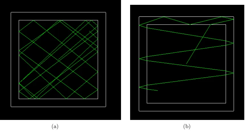
Figure 2.3 shows a cross sectional view of the the pillar with two example photon trajectories. The scintillator pillar is in the center of Figure 2.3 with a 1 mm air gap surrounding the scintillator. A reflector surrounds the air gap.
(a) (b)
Figure 2.3 Cross sectional view of the pillar geometry with two example photon trajectories. (a) An example optical photon trajectory that results in TIR throughout the pillar until self attenuation in the upper right part of the figure. The polished sides of the scintillator are not perfectly smooth which produces slight deviations in the reflected angle. (b) An example of a photon trajectory that escapes the pillar. The photon originates in the center of the pillar, then Fresnel refracts out into the air gap and bounces off the reflector twice. The photon continues to enter and exit the pillar until reaching the photodetector in the bottom of the figure.
of the figure. For the Geant4 simulations, the polished sides of the scintillator were not perfectly smooth which imparted slight angle deviations each reflection; We used a normal distribution with a mean of zero and a standard deviation of 1.3◦ to randomly sample the reflection angle. In the simulation, TIR caused photons to travel large distances (>100 cm) before arriving at the photodetector. Photons emitted from scintillation with little to no velocity in the z-direction exhibit long transit times and a large number (>100) of reflections.
and interact with the reflector. Therefore, we investigated two different types of reflective film models to maximize light collection at the ends of the pillar.
2.1.2.1 Reflector Models
We simulated two types of reflector materials; titanium dioxide (TiO2) paint and enhanced
specular reflector film (ESR) [1]. We simulated each reflector using built in look up tables (LUT) in Geant4:PolishedESR LUT for ESR film andpolishedtioairfor TiO2 [29–31]. The titanium
dioxide paint and ESR film behave as a Lambertian reflector and specular reflector respectively. At incident photon angles exceeding 50◦, TiO2 paint transitions into a hybrid of a specular
reflector and Lambertian reflector [31]. Both reflectors decrease in reflectivity for wavelengths below 400 nm [30, 40] as shown in Figure 2.4(a). The large decrease in reflectivity for the ESR is due to absorption of light below 390 nm which fluoresces at 430 nm [30]. ESR fluorescence was not included in the simulation. Recalling the emission spectra from Figure 2.2, EJ-232Q’s low average wavelength results in poor reflection by TiO2 and ESR. In contrast, the reflectivity
of TiO2 and ESR are high for EJ-204; thus, EJ-204 is a much better choice of scintillator when
using both ESR and TiO2.
We performed simulations in Geant4 for two pillar/reflector configurations. In the simulations, we estimated the collection efficiency for one photodetector. For the first configuration, we directly attached the reflector to the pillar. For the second configuration, the reflector lined the housing walls with a 1 mm gap of air between the scintillator and reflector. We compared each configuration to a base case consisting of a bare scintillator surrounded by air. We simulated a 1 cm x 1 cm x 20 cm EJ-204 pillar using 107 photons emitted isotropically at each position. The results are shown in Figure 2.4(b).
300 350 400 450 500 550 600 Wavelength (nm) 0.0 0.2 0.4 0.6 0.8 1.0 Reflectivity ESR TiO2 (a)
2.5 5.0 7.5 10.0 12.5 15.0 17.5
Scintillation Distance From Photodetector (cm) 0.1 0.2 0.3 0.4 Fraction of light incident on one end of the pillar ESR + 1 mm Air Gap TiO2 + 1 mm Air Gap No Reflector ESR TiO2 (b)
Figure 2.4 (a) Reflectivity of ESR and TiO2 as a function of wavelength. Note the decrease in
reflec-tivity for both reflectors near 400 nm. (b) Simulated reflector study with commonly used reflective materials in detector applications. The emission spectrum of EJ-204 was used. A 1 mm air gap was simulated to allow photons to undergo TIR. The ‘No Reflector’ case consists of an EJ-204 pillar sur-rounded by air.
escape the pillar and are not detected. We see a decrease in collection efficiency as distance increases due to additional escaping photons and to self-absorption of scintillation light.
Titanium dioxide paint with a 1 mm air gap still allows for TIR of scintillation photons, but it diffusely reflects escaping photons back into the pillar that did not undergo TIR. The most likely angle of reflection in the TiO2 paint is parallel to the surface normal of the housing
wall. This explains the decreasing light collection efficiency as scintillation-detector distance increases. However, due to the air gap, the light collection efficiency converges to the ‘No Reflector’ case at large distances. Directly painting the pillar with TiO2 shows a reduction
in collection efficiency after a 2 cm distance. TiO2 has a higher index of refraction than the
scintillator pillar which prohibits TIR [29]. This produces a very poor light collection efficiency for large scintillation-detector distances.
The ESR film and air gap combination exhibits light collection efficiency above 25% at distances up to 13 cm. Again, the collection efficiency converges on the ‘No reflector’ case at large distances (albeit more slowly than the TiO2 + air gap combination). Consequently, we
The reflectivity of ESR film reduces the collection of photons with wavelengths below 390 nm. Figure 2.5 shows the distribution of photon wavelengths for stilbene arriving at the end of the pillar compared to the original emission spectrum. The relative yield is normalized to the amplitude of the emission peak at 382 nm. At short scintillation to photodetector distances, photons with wavelengths >390 nm are more likely to be collected at the end of the pillar after reflection in the ESR film. This increases the amplitude of the peak near 400 nm relative to the 382 nm peak.
350
375
400
425
450
475
500
Wavelength (nm)
0.0
0.2
0.4
0.6
0.8
1.0
Relative Yield (A.U.)
Scintillation Distance to PD (cm) 1 2 3 4 5 6 7 8 9 10 11 12 13 14 15 16 17 18 19 Emission SpectrumFigure 2.5 Collected light spectrum as a function of distance for a stilbene pillar using an air gap and ESR lining the housing walls. The decrease in ESR reflectivity under 400 nm affects the collected light spectrum.
2.1.2.2 Analysis of Optical Light Transport in the Pillar
photons at a distance of 5 cm from the photodetector. All simulated photons started at time zero. Polar and azimuth angle definitions relative to the pillar are shown in Figure 2.6 which will be referenced in later figures.
Figure 2.6 Polar (θ) and azimuth (φ) angles with respect to the pillar geometry.
(a) (b)
Figure 2.7 Histograms of 107 scintillation photons emitted 5 cm away from the photodetector for a 1
cm x 1 cm x 20 cm EJ-204 pillar using a 1 mm air gap and ESR lining the housing walls. (a) Time of arrival of optical photons plotted against the number of direction changes. (b) Time of arrival of opti-cal photons relative to the polar emission angle. Photons only undergo TIR at emission angles below 51◦. Emission angles above 51◦ result in a mixture of photons that escape the pillar and photons that undergo TIR depending on their azimuth emission angle.
the opposing photodetector. There is a possibility that the photons can change direction over multiple reflections and move in the opposite z-direction from slight deviations in the reflected photons exit angle. Again, a majority of the photons arrive at short travel times below 2 ns.
Figure 2.8(a). At azimuth angles around 45◦, 135◦, 225◦, and 315◦, only TIR occurs, regardless of polar emission angle θ. However, the polar angle θdictates how direct the photon’s travel is towards the photodetector. Most angles allow for quick travel to the photodetector indicated by the larger population of counts at a small number of direction changes. Photons that escape the pillar produce counts outside the “comb-like” pattern seen in the figure. The tortuous path traversed by escaping photons increases the number of direction changes before arriving at the photodetector.
(a) (b)
Figure 2.8 Histograms of 107 scintillation photons emitted 5 cm away from the photodetector for
a 1 cm x 1 cm x 20 cm EJ-204 pillar using a 1 mm air gap and ESR lining the housing walls. (a) Direction changes induced from the pillar geometry in relation to the azimuth emission angle. (b) Photons collected at the end of the pillar relative to their polar and azimuth emission angles.
initially emitted at θ >90◦ can reverse direction in the ESR film and interact in the opposite photodetector.
2.1.2.3 Pillar Impulse Response Models
To tabulate pillar impulse response models, we used the same Geant4 optical light simulations discussed in the previous sections. As scintillation photons propagate down the pillar, the pillar’s geometry induces a temporal spread of arrival times at the photodetector. To estimate the distribution of arrival times, we simulated 107 scintillation photons emitted isotropically at time zero in 0.5 cm increments along the pillar length. All scintillation photons were emitted at the center of the pillar in the (x,y) plane. No discernible difference in arrival time was seen for photons emitted at different (x,y) positions. We tabulated the arrival time of each photon that hit the photodetector and binned them to produce a pillar time spread histogram as a function of distance from the photodetector. The “pillar impulse responses” Rpil(t) are shown in Figure 2.9.
0.0
0.5
1.0
1.5
2.0
2.5
3.0
Time (ns)
0
5
10
15
20
25
10
5C
ou
nt
s
(5
0
ps
b
in
s)
Scintillation distance to PD (cm) 1 2 3 4 5 6 7 8 9 10 11 12 13 14 15 16 17 18 19Figure 2.9 Pillar impulse responses (Rpil(t)) for a 1 cm x 1 cm x 20 cm EJ-204 pillar with a 1 mm air
Photons produce a more compact pillar impulse response the closer they originate to the photodetector. At 1 cm away, pillar geometry has a small effect and most incident photons arrive within 0.25 ns of scintillation. However, as the position moves farther away, we observe a much larger spread of arrival times up to 0.75 ns at the farthest distance. Note that the area under each curve decreases as the distance increases. This is due to self-absorption of scintillation light in addition to losses in the ESR film lining the housing walls.
Using the area under the curves at each distance, we calculated the collection efficiency as a function of position in the pillar. We summed the light collected on both photodetectors to obtain a light collection efficiency curve for the pillar. Figure 2.10 shows the efficiency for three different length pillars: 10 cm, 20 cm, and 50 cm. As expected, the highest efficiency is seen for a 10 cm pillar and the lowest is seen for a 50 cm pillar.
20 10 0 10 20
Distance From Center of Pillar (cm) 0.40
0.45 0.50 0.55 0.60 0.65
Light Collection Efficiency
10 cm 20 cm 50 cm
Figure 2.10 Light collection efficiency using both photodetectors for 10 cm, 20 cm, and 50 cm pillars. Higher collection efficiencies are seen for shorter pillars; there is less chance absorption in the scintilla-tor or ESR film.
2.11.
0.0 2.5 5.0 7.5 10.0 12.5 15.0 17.5 20.0 Time (ns)
10
010
110
210
310
410
5Frequency (cts)
0.5 cm wide 1.0 cm wide
Figure 2.11 Photon arrival time histogram for a 20 cm long EJ-204 pillar with different widths. 1.0 cm width slightly increases the time spread of scintillation photons.
2.1.3 Photodetector Impulse Response and Transit Time Spread
We simulated the responses of three different photodetectors of interest. We required photodetec-tors to have a small form factor and the ability to be used in arrays or to have pixelated anodes. The three photodetectors we chose to model were an MCP-PM, an SiPM, and an MA-PMT.
One major difference between the three photodetectors is the impulse response Rimp(t); see Figure 2.12. We modeled the photodetector impulse response using Equation 2.3.
Rimp(t) = [e−t/τf −e−t/τr]h(t) (2.3)
0 10 20 30 40 Time (ns) 0.00 0.01 0.02 0.03 Relative Yield (A.U.) SiPM MAPMT MCPPM (a)
300 350 400 450 500 550 600
Wavelength (nm) 0.0 0.1 0.2 0.3 0.4 QE or PDE SiPM MAPMT MCPPM (b)
Figure 2.12 (a) Photodetector impulse response (Rimp(t)) to charge carriers. The area under each
waveform is normalized to unity. The MCP-PM and MA-PMT both have a compact time response compared to the silicon photomultiplier. (b) The conversion efficiency of optical light to charge carrier as a function of wavelength for each photodetector.
Table 2.2 Modeled photodetector properties [23, 25, 28]
Photodetector Rise Time (ns) Fall Time (ns) TTS (ns)
MCP-PM 0.4 0.6 0.047
SiPM 0.3 12 0.115
MA-PMT 0.4 0.8 0.17
times were taken from fits to the MCP-PM single photoelectron responses shown in Chapter 4. The time The SiPM has an impulse response that includes a fast rise time of 0.3 ns and a slower fall time of 12 ns [28]. Tabulated photodetector properties are shown in Table 2.2.
The wider the photodetector impulse response, the larger the spread of charge carrier collection over time. Recent advancement in SiPM technology now provides a “fast output” which uses approximately 2% of the energy deposited for the signal. This creates a faster rise and fall time of the output signal. However, with only 2% of the signal being collected in the fast output, it will be subject to large fluctuations from small charge collection. So, we did not model the fast output; all results are based on the standard SiPM output impulse response. In these simulations, no electron multiplication was modeled because it does not contribute significantly to the random fluctuations in charge collection.
SiPMs can exhibit up to 50% PDE depending on photon wavelength and the overvoltage applied to the photodetector [28]. Increasing the overvoltage increases the PDE, but it also increases crosstalk between microcells of the SiPM. Crosstalk can approach to 22% for the modeled SiPM. For this analysis, we assumed an operating overvoltage of 2.5 volts which corresponds to 5% crosstalk level and the PDE shown in Figure 2.12(b). Crosstalk and overvoltage were not modeled for these simulations. The QE/PDE for each photodetector is shown in Figure 2.12(b). The photodetector with the highest conversion efficiency is the SiPM at approximately double that of the MCP-PM over all wavelengths. A larger PDE will lead to an increased number of charge carriers in the photodetector per incident photon.
All three scintillator emission spectra shown in Figure 2.2 match well with the peak QE/PDE for the photodetectors. EJ-204 mostly emits photons above 400 nm aligning with the peak PDE of the SiPM. The effect seen in Figure 2.5 for a stilbene scintillator using an ESR film will result in a greater number of charge carriers in an SiPM. The wavelength distribution of collected light is skewed toward the higher PDE region of the SiPM.
Transit time spread (RT T S(t)) is the temporal spread of charge carriers during the multi-plication process within the photodetector. For simplicity, we modeled the transit time spread (TTS of the photodetector as a Gaussian distribution shown in Figure 2.13. The transit time spread (given as 1σ) in all photodetectors is relatively small: 50 ps for the MCP-PM, 115 ps for the SiPM, and 170 ps for the MA-PMT [23, 50].
2.1.4 Constructing Nominal Responses
0.4
0.2
0.0
0.2
0.4
Time (ns)
0
2
4
6
8
Intensity (A.U.)
SiPM MAPMT MCPPMFigure 2.13 Transit time spread (RT T S(t)) models for an MCP-PM, MA-PMT, and SiPM
shows a stilbene pillar using an SiPM and the bottom of the figure shows an EJ-204 pillar using an MCP-PM. The slow fall time of both stilbene and the SiPM result in an elongated decay time for the nominal response. As stated previously, we will compare the nominal responses to simulated observed responses to estimate scintillation location, scintillation time, and proton recoil energy in the pillar.
0 5 10
Yield (Units Arb.)
Stilbene / SiPM
0 10 20 30 40 50 60
Time (ns) 0 20 40 Yield (Units Arb.) EJ204 / MCPPM Scintillation distance to PD (cm) 1 2 3 4 5 6 7 8 9 10 11 12 13 14 15 16 17 18 19
2.2
Observed Responses
Observed responses are constructed by randomly sampling from the nominal responses. We created observed responses using a subset of the responses convolved in Equation 2.1. Initially, we convolved each pillar response function with the time response of the scintillator (shown in Equation 2.4) to produce “scintillation pillar responses” (RSP(t)).
RSP(t) =Rscint(t)∗Rpil(t) (2.4)
We tabulated the scintillation pillar responses at 0.5 cm increments in the z-dimension along the pillar and interpolated between the increments to obtain scintillation pillar responses at any location along the pillar. Scintillation pillar responses estimate the time of arrival at the photodetector and collected scintillation light wavelengths for that specific scintillator.
In simulation, we know the proton recoil energy of interactions. Therefore, we can determine the expected number of scintillation photons produced in each interaction, given the scintillator’s luminosity. As previously mentioned, protons do not exhibit a linear relationship of proton recoil energy to light production due to quenching interactions. These quenching interactions reduce the amount of scintillation light created. The luminosity is multiplied by the collection efficiency at that scintillation position to estimate the number of photons that arrive at the face of the photodetector. Not all photons incident on the photodetector create a charge carrier. Each incident photon is randomly assigned a wavelength from the scintillation pillar response. Then, using the wavelength dependent QE/PDE shown previously in Figure 2.12(b), we randomly sample if each photon will produce a charge carrier. The number of charge carriers created is shown in Equation 2.5
nCC =LO(Ep)·L·LC(z)·P D(λ) (2.5)
Ep is the proton recoil energy (MeV), L is the luminosity of the scintillator (scintillation photons/MeVee), LC(z) is the collection efficiency as a function of position in the scintillator (collected photons/emitted photons), andP D(λ) is the wavelength dependent quantum efficiency or photon detection efficiency (charge carriers/incident photon). We randomly sampled the number of charge carriers from a Possion distribution with a mean ofnCC. Charge carrier arrival times were randomly sampled from the scintillation pillar response.
Photodetectors are positioned on opposite sides of the pillar. This provides a correlated pair of responses for each scintillation event. For example, consider a 20 cm length pillar. If scintillation occurs 5 cm away from the left photodetector, the same scintillation photons emerge 15 cm from the right photodetector. Therefore, both photodetector responses can be used to estimate the position of scintillation along the length of the pillar.
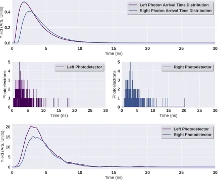
Figure 2.15 illustrates the observed waveform simulation process. The first step involves calculating the pair of scintillation pillar response functions at the true distance to the left and right photodetector shown in the top of the figure. Using the pair of scintillation pillar responses, we randomly sample charge carrier arrival times. The number of charge carriers sampled is dictated by Equation 2.5 and shown in the middle of Figure 2.15. We smeared each charge carrier arrival by the transit time spread characteristic to each photodetector. Finally, to estimate the observed output waveform, we convolved the charge carrier arrival time histories shown in the middle of the figure with the photodetector impulse response shown in Figure 2.12. This operation spreads out the charge carriers over multiple time bins. Commercially available fast digitizers based on switched capacitor arrays can sample waveforms every 200 ps [4, 52, 59]. Therefore, we binned our observed waveforms in 200 ps intervals. The observed photodetector output waveform is shown at the bottom of Figure 2.15 for both the left and right photodetector.
0
5
10
15
20
25
30
Time (ns)0.0
0.2
0.4
Yield (Arb. Units) Left Photon Arrival Time Distribution Right Photon Arrival Time Distribution0
5
10
15
20
25
30
Time (ns)
0
1
2
3
4
5
Photoelectrons Left Photodetector0
5
10
15
20
25
30
Time (ns)
0
1
2
3
4
5
Photoelectrons Right Photodetector0
5
10
15
20
25
30
Time (ns)
0
5
10
15
20
Yield (Arb. Units) Left Photodetector Right PhotodetectorCHAPTER
3
SCINTILLATION POSITION,
SCINTILLATION TIME, AND PROTON
RECOIL ENERGY ESTIMATION
refer to the size in (x,y) dimension. Using our method, interaction position estimation in the (x,y) coordinates is not possible within a single pillar. So, when we back-project incident neutron cones (in Chapter 5), we set the estimated scintillation position in (x,y) at the center of the pillar illuminated with scintillation light. Pillars have an aspect ratio of one in the (x,y) plane for simplicity, i.e. they have the same width in both the x and y direction. There are four main steps to the simulation.
1. Simulate scintillation photon emission
(a) Randomly select the number of scintillation photons from a Poisson distribution with a mean equal to proton recoil energy times the luminosity corrected for quenching
(b) Scintillation photon timing is randomly sampled from the scintillator time response function
(c) Scintillation photon wavelength is randomly sampled from the scintillator emission spectrum
2. Simulate light collection efficiency
(a) Randomly select the number and time of arrival of scintillation photons on the photodetectors from the optical pillar response function
3. Model charge carrier production in the photodetectors
(a) Randomly sample the number of charge carriers generated at the photodetectors based on the wavelength dependent MCP-PM/MA-PMT quantum efficiency and SiPM photon detection efficiency
(b) Randomly sample the time of arrival of charge carriers from the photodetector transit time distribution
4. Apply Poisson maximum likelihood estimation to fit the randomly sampled charge carrier arrival time history (observed response) with the nominal arrival time history where scintillation position, scintillation time, and proton recoil energy are unknown variables
Steps 1-3 produce observed responses for each simulated event as described in Chapter 2. We fit the nominal responses to the observed responses to get the best estimate of the parameters in the fourth step. We analyzed 10,000 charge carrier waveforms simulated using the preceding steps for each photodetector/scintillator combination. The uncertainties are the sample root mean squared (RMS) error for those 10,000 simulations which account for most of the relevant effects, excluding anisotropy in luminosity and optical photon transport in stilbene (where the average behavior of stilbene was modeled).
We will show the best scintillator and photodetector combination is EJ-204/MA-PMT. The compact charge carrier distribution in the MA-PMT and the fast, bright scintillation of EJ-204 allows for the most precise position estimate (<1 cm RMS error), proton recoil energy estimate (<50 keV RMS error) and scintillation time (<100 ps RMS error) for proton recoil energies above 1 MeV; these results are described in detail in Section 3.3 and illustrated in Figures 3.3, 3.4 and 3.5. The precision of position reconstruction is dependent upon where in the pillar the scintillation occurred; it is less precise in the center of the pillar due to the low total collection efficiency at that location. Lastly, we examine the scintillation position, time, and proton recoil energy reconstruction precision as a function of energy from 0.5 to 3 MeV using the EJ-204/MA-PMT combination.
3.1
Alternative Methods to Estimate Scintillation Position
in time of arrival of the observed waveforms.
Previous work [12, 32, 41] performed measurements using pillar scintillators to produce position sensitive detectors. They used the intensity of light on opposing photodetectors to estimate the position of interaction within the pillar. In [12], the experiment utilized gamma-ray Compton scatter instead of neutron elastic scatters. As discussed earlier, protons do not exhibit a direct proportionality between energy deposited and light created in the scintillator. Scintillation position estimates are less precise for neutron scatter events due to the lower intensity of scintillation light produced from a proton recoil compared to Compton scatter.
Other works [32, 37, 41] have used the time of arrival of the observed waveforms at the ends of a pillar to estimate scintillation location. The time of arrival of waveforms is measured using constant fraction discrimination (CFD). When an interaction occurs in the center of the pillar, the distance the scintillation photons have to travel is the same, thus, the time of arrival of the two waveforms will be approximately the same. If the interaction occurs nearer to one of the photodetectors than the other, there will be a delay in the arrival time for the distant photodetector.
We used the same optical light transport model discussed in Chapter 2 to simulate the transit of scintillation light throughout the pillar. We estimated scintillation position using both alternative methods to investigate their precision and accuracy. The simulation consisted of a 1 cm x 1 cm x 20 cm EJ-204 scintillator pillar with a 1 mm air gap. An enhanced specular reflector film surrounded the air gap to reflect escaping photons back into the scintillator. MCP-PMs were attached on the left and right sides of the pillar.
the arrival time at the right photodetector (tR) producing a negative time difference when the interaction is on the left side of the pillar. Conversely, scintillation events on the right side of pillar have negative charge ratios and positive time differences.
10 5 0 5 10
Distance from Center of Pillar (cm) 1.0 0.5 0.0 0.5 1.0 tL tR (n s) Time of Arrival Difference Log Ratio of Charge 0.75 0.50 0.25 0.00 0.25 0.50 0.75 ln (QL / QR ) (a)
0.5 1.0 1.5 2.0 2.5 3.0
Proton Recoil Energy (MeV) 0.5 1.0 1.5 2.0 2.5 3.0 Position RMS Error (cm) Time of Arrival Difference Log Ratio of Charge (b)
Figure 3.1 Scintillation position estimates using relative light intensity and time of arrival. Simulation performed using a 1 cm x 1 cm x 20 cm EJ-204 organic plastic scintillator with a 1 mm air gap and an enhanced specular reflector. (a) Log ratio of charge collected and time of arrival difference curves cre-ated using nominal responses to get an average at each position along the pillar. Error bars correspond to the uncertainty in relative timing and intensity for a 2 MeV proton recoil. (b) Scintillation position estimate RMS errors using both methods.
We simulated 10,000 proton recoil events in 0.5 cm increments spanning the pillar to estimate the precision of the two methods with proton recoil energies ranging from 0.5 MeV to 3 MeV. At each position, we calculated the intensity of light incident on the left and right photodetector in addition to the time of arrival difference. We calculated the time of arrival using constant fraction discrimination with a 50% fraction. We estimated the scintillation position using the average log ratio curve and timing difference curve in Figure 3.1(a) and calculated the RMS error. The results are shown in Figure 3.1(b).