ABSTRACT
GAINEY, KEVIN W. Determination of Possible Wetland Mitigation Sites Using
NC-CREWS and an Integer Linear Programming Formulation. (Under the direction of
Joseph P. Roise).
The objective of this project was to develop an optimization model for wetland
mitigation site selection using a geographic information system for rating wetlands and
traditional operations research methodologies. This project was conducted using a GIS
based wetland assessment procedure entitled North Carolina Coastal Region Evaluation
of Wetland Significance (NC-CREWS) developed by the North Carolina Department of
Environmental Resources’ Division of Coastal Management (DCM). NC-CREWS rates
possible mitigation sites by the wetland functions they could perform if fully restored.
Using this component of NC-CREWS, a conceptual model to optimize the selection of
restoration sites based on their functions was developed and tested on a small,
fabricated example to test workability. This model was adapted to include possible
restoration site ratings from an actual watershed in Craven County, NC, provided by
DCM. The 0-1 integer programming model that was developed was tested using trials
to address issues of problem size, functional unit level required, and order of sites used
in the model. Of the 180 tests, all but 37 reached an optimal solution by 200 million
iterations of a branch-and-bound algorithm. The problem size and number of functional
units required had little impact on the solution time. The ordering of sites as supplied to
model it is possible to derive a list of possible mitigation sites to use for improving field
DETERMINATION OF POSSIBLE WETLAND MITIGATION SITES USING NC-CREWS AND AN INTEGER LINEAR
PROGRAMMING FORMULATION
by
KEVIN WAYNE GAINEY
A thesis submitted to the Graduate Faculty of North Carolina State University
In partial fulfillment of the Requirements for the Degree of
Master of Science
FORESTRY
Raleigh
1998
APPROVED BY:
To Jerry and Pat Gainey
Without their constant encouragement, advice, and all-round support, I would not be where I am today.
Thanks for always helping me find the answers, even if the most common words I heard as a child were
BIOGRAPHY
Kevin Wayne Gainey was born October 24, 1973 in Concord, North Carolina. He
received two years of high school education at A.L. Brown High School in Kannapolis,
NC, and graduated from the North Carolina School of Science and Mathematics in
Durham in 1992.
Kevin received the Bachelor’s of Science degree in Forest Management from North
Carolina State University in May of 1996. He started his research in July of 1996.
Kevin received a Center for Transportation and the Environment Fellowship in May of
1997 and was also rewarded a Philip Morris Graduate Scholarship.
The author currently resides in Raleigh, NC and works for the the North Carolina
ACKNOWLEDGEMENTS
I am indebted to the entire NCSU College of Forest Resources for the support I have
received during both my undergraduate and graduate careers. Special thanks to Drs.
Joseph Roise, Hugh Devine, Ted Shear, and Heather Cheshire for their professional and
personal support throughout this endeavor.
I would like to especially thank the people who have seen me struggle the most with
this project from its inception… my roommates: James Jong, Ryan Boyles, Steve
Hughes, Mark Nippert, and Taylor Roberts. Thanks for always helping me “focus” on
my work and avoid the distractions of Monday Night Football and ACC Basketball!!!
Thanks also to everyone else who helped along the way: Casey Bianco, Sean Cassidy,
Patricia Festin, Roger Mabry, Alex Miller, John & Jennifer Nicosia and Chaffee Viets.
A very special thank-you goes to Sabrina Alvarez for encouraging me over the past year
when things have been rough. Your friendship means more than you will ever know. I
TABLE OF CONTENTS
LIST OF TABLES… … … ..vi
LIST OF FIGURES… … … vii
PREFACE… … … ..… … … ...viii
CHAPTER 1: Analysis of Road Locations in Wetlands and Mitigation Site Selection Introduction… … … ..2
Description of the Model… … … ..3
NC-CREWS Functions… … … .… 3
Terrestrial Wildlife Habitat… … … .… ..3
Nonpoint Source Pollution Reduction… … … … .… .4
Floodwater Storage… … … .… ..5
Methods and Assumptions… … … .… ...5
The Model… … … .… … 7
An Example Using Habitat Functions… … … .… … ..9
Discussion and Conclusions… … … .… ...12
References… … … .… ..14
CHAPTER 2: Determination of Possible Wetland Mitigation Sites Using NC-CREWS And an Integer Linear Programming Formulation Introduction… … … .16
Model Development… … … ....18
Results… … … ..… 25
Discussion and Conclusions… … … .… 27
LIST OF TABLES
Table 1.1 Ratings Assigned to Wildlife Habitat Parameters 4
Table 1.2 Ratings Assigned to Nonpoint Source Pollution 4 Parameters
Table 1.3 Ratings Assigned to Floodwater Storage Parameters 5
Table 1.4 Characteristics of Example Watershed 10
Table 1.5 User Defined Constants for Test Scenario 11
Table 1.6 Functional Units Gained from Possible Mitigation 12 Site Combinations
Table 2.1 Tests for Use in LINDO Model 23
Table 2.2 Number of Iterations Comparing Use of Tolerance 26 For Wetlands Sorted by ID with a Target Mitigation
Of 100 FU
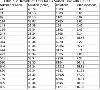
Table 2.3 Results of Tests for ID Sorted Trial with 100 FU 30
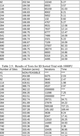
Table 2.4 Results of Tests for ID Sorted Trial with 500 FU 31
Table 2.5 Results of Tests for ID Sorted Trial with 1000 FU 31
Table 2.6 Results of Tests for Perimeter Sorted Trial with 100 FU 32
Table 2.7 Results of Tests for Perimeter Sorted Trial with 500 FU 32
Table 2.8 Results of Tests for Perimeter Sorted Trial with 1000 FU 33
Table 2.9 Results of Tests for Random Sorted Trial with 100 FU 33
Table 2.10 Results of Tests for Random Sorted Trial with 500 FU 34
LIST OF FIGURES
Figure 1.1 Simplified arrangement of land units in a watershed 9 where road impacts will require mitigation
Figure 1.2 Example watershed with added road which requires 10 mitigation
Figure 2.1 Comparison of use of tolerance with no use of 26 tolerance
Figure 2.2 Number of sites vs. iterations for ID ordering 35
Figure 2.3 Number of sites vs. iterations for Perimeter ordering 36
Figure 2.4 Number of sites vs. iterations for Random ordering 37
Figure 2.5 Number of sites vs. time for ID ordering 38
Figure 2.6 Number of sites vs. time for Perimeter ordering 39
Preface
Wetlands are a part of the natural landscape and have been the subject of countless
scientific and legislative debate. Evolving from this debate, federal and state policies
require that impacts to or degradation of a wetland be mitigated for, meaning wetland
losses must be replaced (most notably, Section 404 of the Federal Clean Water Act).
The process of mitigation can be ad hoc, in that there is no good tool for finding
possible mitigation sites where the wetland replacement is based on functions instead of
acreage (Bledsoe et al. 1997, Richardson 1994). Current practices within the 404
permit process does not distinguish between high and low quality wetlands when
considering permit approval (Sutter & Wuenscher 1997) and it is up to the permit
applicant to select sites for use as mitigation (Bledsoe et al. 1997). The applicant is
often not ecologically qualified, and in the interest of time and money, settles for
available land with little concern for the quality of wetlands that will be restored
(Bledsoe et al. 1997).
Wetlands were once pervasive in the coastal plain of North Carolina but draining and
development have converted many sites to agricultural fields, pine plantations, road
corridors, and urban areas (Johnston 1994, Sutter & Wuenscher 1997). Because the
societal and ecological values of wetlands have been emphasized in recent decades,
there is a desire to better protect existing wetlands and improve the wetland restoration
process. Wetland restoration is simply taking an area that was once a wetland but has
vegetation, hydrology, and some soil characteristics to pre-disturbance levels, if
possible.
Population growth, which requires larger transportation systems, extends humans’
impact on the environment. Joy Zedler of the Pacific Estuarine Research Laboratory at
San Diego State University claims highway agencies are one of the largest destroyers of
wetlands due to corridor placement in low, flat areas where natural wetlands once
flourished (ENR 1994). Highways located in floodplains can alter hydrologic
relationships because of floodplain constriction and changes in flow rates due to
roadbeds and culverts (Walbridge & Lockaby 1994). These changes can alter the
energy signature of the wetland, precipitating a change in species composition and
distribution. Walbridge and Lockaby also state that in time the biogeochemical
input/output relationships re-establish. Depending on the amount of change, the overall
capability of the wetland to perform the impacted functions may change. These
changes in energy signatures can lead to slower moving water or stagnation. Conner
and Day showed that net primary productivity is reduced as surface waters become
more stagnant (1982) and Johnston recorded a similar decrease in southeastern
bottomland forests (1994). These impacts affect the level at which a wetland performs
various functions.
The North Carolina Department of Environmental and Natural Resources’ Division of
Wuenscher 1997). This assessment method, titled North Carolina Coastal Region
Evaluation of Wetland Significance (NC-CREWS), is a procedure based on spatial data
layers contained in a geographic information system (GIS). NC-CREWS provides a
method for rating existing wetlands as well as possible mitigation sites. NC-CREWS
uses National Wetland Inventory maps and three classes from the hydrogeomorphic
classification system developed by Mark Brinson (Brinson 1993) for defining and
classifying wetlands. Using NC-CREWS ratings and a technique to optimize the
selection of mitigation sites could provide a tool to improve the compensatory
mitigation of wetland functions.
The need for a quantitative tool allowing transportation and mitigation planners to select
possible restoration sites led to a research grant sponsored by the Center for
Transportation and the Environment. The following chapters describe an approach to
combine NC-CREWS with a linear programming model to enhance the restoration site
selection process after a transportation project or other construction effort adversely
impacts wetlands. Chapter 1 focuses on the development of a conceptual model and a
simple test scenario. Chapter 2 refines the model and includes actual NC-CREWS
ratings and tests the resulting model on a sample watershed using a series of trials.
REFERENCES
Bledsoe, Brian P. et al. 1997. A Geographic Information System for Targeting Wetland Restoration. North Carolina Department of Environment and Natural Resources. Raleigh, NC.
Brinson, M. M. 1993. A Hydrogeomorphic Classification for Wetlands. Wetlands Research
Conner, W.H. and J.W. Day, Jr. 1982. The ecology of forested wetlands in the southeastern United States. 69-87. In B. Gopal, R.E. Turner, R.G. Wetzel, and D.F. Whigham (eds). Wetlands Ecology and Management. National Institute of Ecology and International Scientific Publications, Jaipur, India.
ENR. 1994. Can Agencies Pass Swampbuilding 101? Engineering News Review, 18 Apr: 16.
Johnston, Carol A. 1994. Cumulative Impacts to Wetlands. Wetlands. 14(1):49-55.
Richardson, Curtis J. 1994. Ecological Functions and Human Values in Wetlands: A Framework for Assessing Forestry Impacts. Wetlands. 14(1):1-9.
Sutter, L.A. and Wuenscher, J.E. 1997. NC-CREWS: North Carolina Coastal Region Evaluation of Wetland Significance, North Carolina Department of
Environment Resources, Raleigh, NC.
CHAPTER 1
INTRODUCTION
The purpose of this work was to find a way to improve the transportation planning
process by including wetland functions in a spatial analysis tool. Wetland functions
are the ecological processes that occur in these systems. For example, the ability of a
wetland to provide nesting habitat for waterfowl is a function. Groundwater recharge,
pollutant removal, and floodwater storage are other wetland functions. These
functions should not be used as synonyms for wetland values, the importance that
society assigns to wetland functions. A wetland may play a large role in removing
sediment and pollutants from a city’s water supply, and therefore be valuable to the
city. However, wetlands with the same functions but not directly affecting the water
supply may not be as valuable to the city.
Whenever a transportation or other construction project detrimentally impacts
wetlands, those impacts must be mitigated. Wetlands mitigation is the process of
replacing the wetland functionality that was destroyed. This is most often done
through wetland restoration, the process of reestablishing a wetland that has been
converted. Policy defined ratios exist that control the number of acres that must be
mitigated and are dependent on the type of mitigation being performed. However, the
North Carolina Division of Coastal Management has cited this process as a contributor
to failure of mitigation because wetland functions are not specifically considered in
DESCRIPTION OF THE MODEL
NC-CREWS Functions
NC-CREWS looks at a variety of wetland functions, but only three were considered in
this first version of the model. The functions considered are terrestrial wildlife habitat,
nonpoint source pollution reduction, and floodwater storage. Each function has a
series of parameters which are combined to give each wetland unit in the GIS an
overall rating for each function. The wetlands are rated High, Medium, or Low for
each function being considered. The database developed by DCM contains these
ratings for existing wetlands. Because this model also looks at sites that could be
converted back to wetlands, these functional ratings must be calculated for each
combination of land units chosen as satisfying the mitigation requirements. At the
time of model development DCM was working on a method for rating possible
restoration sites. Since this information was not available, a similar method was used
for the purposes of this model that was based on the NC-CREWS method of rating
existing wetlands. The rating strategy used for the three functions below comes
directly from Sutter and Wuenscher (1997).
Terrestrial Wildlife Habitat
This function is rated on the quality of habitat provided for terrestrial wildlife. The
parameters considered are interior size, percent surrounding habitat that is natural
To calculate interior habitat, a buffer zone of 100 meters around the perimeter is
subtracted from the total area (Sutter & Wuenscher 1997). The rating strategy for
wildlife habitat parameters is shown in Table 1.1.
Table 1.1: Ratings assigned to wildlife habitat parameters
Parameter High Rating Medium Rating Low Rating
Interior Size > 74 acres 0 - 74 acres None % Surrounding
Habitat
> 50% wetlands < 50% wetlands Isolated from other wetlands
Wildlife Corridor > 600 feet < 600 feet Isolated from natural habitat
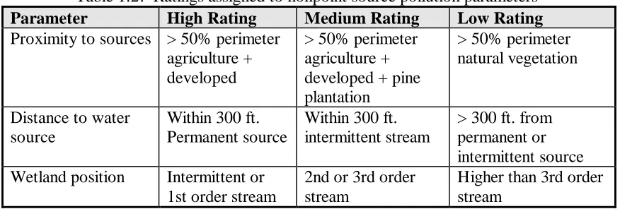
Nonpoint Source Pollution Reduction
Three parameters of the nonpoint source rating system were considered. First, the
proximity to agriculture, developed land, pine plantation, and natural vegetation are
considered using the percent of surrounding habitat as the criteria. Second, the
distance from a water source is used. Third, the position of the wetland relative to
stream orders is used. Table 1.2 summarizes the rating scheme.
Table 1.2: Ratings assigned to nonpoint source pollution parameters
Parameter High Rating Medium Rating Low Rating
Proximity to sources > 50% perimeter agriculture + developed
> 50% perimeter agriculture + developed + pine plantation
> 50% perimeter natural vegetation
Distance to water source
Within 300 ft. Permanent source
Within 300 ft. intermittent stream
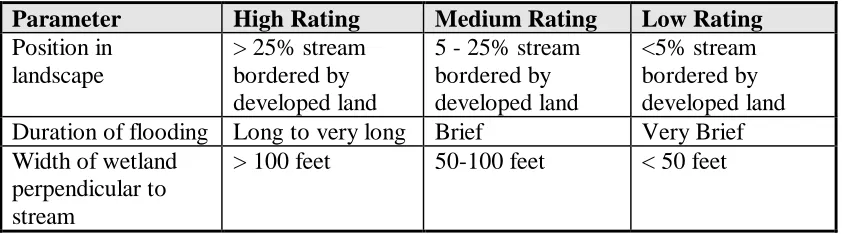
Floodwater Storage
The position of the wetland in the landscape, the duration of flooding, and the width of
the wetland perpendicular to the stream are the parameters considered for rating the
floodwater storage capacity of a wetland. Table 1.3 summarizes floodwater storage
rating criteria.
Table 1.3: Ratings assigned to floodwater storage parameters
Parameter High Rating Medium Rating Low Rating
Position in landscape
> 25% stream bordered by developed land
5 - 25% stream bordered by developed land
<5% stream bordered by developed land Duration of flooding Long to very long Brief Very Brief Width of wetland
perpendicular to stream
> 100 feet 50-100 feet < 50 feet
Methods and Assumptions
To make the NC-CREWS rating method work in a model, values had to be assigned to
the rankings of High, Medium, and Low. The rankings were treated as indices and
were assigned integer values of 1,2, and 3 (Low, Medium, and High). The acreage of
the wetland is multiplied by the rating for each parameter in each functions and
combined to produce a cumulative, numerical ranking that represents functional units
supplied by the wetland. NC-CREWS does not use a straight summation of parameter
ratings to obtain the function ratings. This method was used here to simplify the
model for the purpose of providing a clear example of applying a linear programming
The generalized steps that the model employs are:
1. The total functional units existing in a watershed where a road is planned are
calculated using the NC-CREWS GIS procedure.
2. The user indicates a transportation corridor by adding the link to an existing road
network.
3. For links impacting wetlands, the functional units of the watershed are recalculated
to measure the number of units lost to the road addition.
4. The mixed integer model is run to find the optimal combination of land units to be
converted to mitigation sites.
In order to make a workable model based on NC-CREWS that would be usable in a
GIS environment, several key assumptions have been made for this simple scenario:
1. All of the parameters and functions are equally weighted. Future models
should allow the user to assign weights to different functions to better meet
actual needs.
2. There is no requirement that units removed by a corridor at the parameter level
must be replaced by the same parameters in the mitigation sites. Only the total
number of units at the function level must be replaced. For example, the
number of habitat units destroyed must be replaced by habitat units, but the
units restored from interior size parameter do not have to match those
destroyed for the same parameter by the road.
integer programming requirement. Without this assumption the model would
be a great deal easier to solve, but it might not correctly represent the wetland
ratings.
The Model
Following the above procedure and using the listed assumptions, the linear
programming model has the form:
Maximize ∑(AiXi(FHab x RHabi + FNPS x RNPSi + FFS x RFSi - c)) – (1)
CRoad - (FHab)(HLoss) - (FNPS)(NPSLoss) - (FFS)(FSLoss)
Subject to RHabATX ≥ HLoss (2)
RNPSATX ≥ NPSLoss (3)
RFSATX ≥ FSLoss (4)
CRoad + cATX ≤ CMax (5)
Xi∈ [0,1] (6)
Where Ai = acreage for land unit i for i = 1...n with n land units in study area
Xi = [0,1] decision variable to convert land unit i to wetland, i = 1 to n
FHab = scalar conversion factor of a habitat functional unit to dollars
FNPS = scalar conversion factor of a nonpoint source functional unit to
dollars
FFS = scalar conversion factor of a floodwater storage functional unit to
dollars
RHabi = sum of ratings for habitat parameters, integer in [3 ..9], for site xi
RNPSi = sum of ratings for nonpoint source parameters, integer in [3 ..9]
for site xi
RFSi = sum of ratings for floodwater storage parameters, integer in
[3..9], for site xi
c = cost per acre of converting land to wetland CRoad = cost of constructing road corridor
HLoss = habitat functional units lost to road corridor
NPSLoss = nonpoint source functional units lost to road corridor
FSLoss = floodwater storage functional units lost to road corridor
Equation (1) serves as the objective function and denotes that the goal is to maximize
the financial return of restoring wetlands based on the associated dollar values for each
function and the cost of restoring the sites. Equations (2), (3), and (4) denote the goal
of restoring at least as many functional units as were destroyed (see assumption
number 2 on page 6). Equation (5) states that the cost of the road and the cost of
restoring sites may not exceed some specified project maximum. Equation (6) denotes
the use of a 0-1 integer programming formulation where the decision variables take on
values of 1 for choosing a site to restore and 0 for not selecting site Xi.
The constraints for nonpoint source (3) and floodwater storage (4) are based only on
the total area of the land units when calculating functional units. However, when
calculating functional units for interior habitat, if adjacent land units are chosen, the
amount of interior habitat will increase because portions of the 100 meter buffer will
become interior space. Therefore, for each iteration of the program, RHab must be
recalculated. This would ideally be done by the GIS database accompanying the
NC-CREWS system, but it is done by hand in the example in the next section.
The last four terms of the objective function (1) are costs incurred from road
construction and do not depend on the combination of possible mitigation sites. For a
single road corridor alternative, these terms may be dropped from the objective
function and the maximum mitigation return can be calculated. The terms have been
An Example Using Habitat Functions
The following example uses the above model with only the habitat function to
determine an optimal mitigation combination for a given road corridor. The resulting
model formulation includes only equations (2), (5), and the terms from (1) pertaining
to FHab, RHab, and HLoss. Visual display of nonpoint sources and floodwater storage
becomes difficult without a GIS since hydrology and land use data layers must be used
together. The intent is to show how the model can be applied to a given scenario and
the steps that an automated GIS approach would use.
Figure 1.1 shows the pre-road watershed and Table 1.4 contains the corresponding
acreage information. After unavoidably placing part of a road through an existing
wetland (Fig. 1.2) mitigation combinations must be calculated.
Table 1.4. -- Characteristic of example watershed
Land Unit Land Use/ Land Type Total Acres Interior Acres
X1 Wetland 150 80
X2 Pine Plantation 62.5 22.5
X3 Pine Plantation 70 25
X4 Pine Plantation 30 5
X5 Pine Plantation 62.5 22.5
Figure 1.2: Example watershed with added road which requires mitigation.
The road added to the watershed splits X1 into two new land units, creating X6. X6
has an area of 22.5 acres, with interior space occupying 10 acres. The shaded area
represents the 100-meter buffer around the road where the impacts occur. The
undisturbed watershed contained 750 functional units. Adding the road destroyed 390
habitat functional units (calculated from the impact area of 82.5 acres and the values in
Table 1.5: User defined constants for test scenario.
Constant Value ($)
FHab 2
FNPS 2
FFS 2
c 20
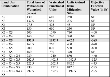
For each combination of the possible mitigation sites, the number of habitat functional
units restored and the accompanying objective function value was calculated . When
using the algorithm with only the habitat function, the optimum combination of land
units to restore to wetlands is X2 and X5. Table 6 shows the functional units and
mitigation returns possible from all combinations of X2, X3, X4, and X5. X1 and X6
remained wetland and therefore cannot be used for mitigation credit. The alternatives
in Table 1.6 where the value for “Units Gained From Mitigation Sites” are less than
390 are not valid because they would violate equation (2) of the model.
This example shows the optimum combination of mitigation sites in terms of financial
outlay. Using the figures given in Table 1.5, meeting the constraints results in a
financial loss. Depending on the choices of F Hab, FNPS, and FFS, it is possible that the
optimum objective function value could have been positive for this scenario. These
financial values were arbitrarily chosen and would be different for various interest
Table 1.6. -- Functional Units Gained from Possible Mitigation Site Combinations.
Land Unit Combination
Total Area of Wetlands in Watershed (acres) Watershed Functional Units Units Gained from Mitigation Sites Objective Function Value (in $)*
X2 130 610 250 NF
X3 137.5 565 205 NF
X4 97.5 405 45 NF
X5 130 610 250 NF
X2 + X3 200 1090 730 -400
X2 + X4 160 740 380 NF
X2 + X5 192.5 1052.5 692.5 -385
X3 + X4 167.5 760 400 -670
X3 + X5 200 890 530 -800
X4 + X5 160 730 370 NF
X2 + X3 + X4 230 1240 880 -460
X2 + X3 + X5 262.5 1402.5 1042.5 -525
X2 + X4 + X5 222.5 1202.5 842.5 -445
X3 + X4 + X5 230 1172.5 812.5 -595
X2 + X3 + X4 + X5
292.5 1552.5 1192.5 -585
*
Does not include last four terms of the objective function which are constants. NF denotes a nonfeasible solution.
DISCUSSION AND CONCLUSIONS
Given the simplicity of the scenario and the stated assumptions, the model formulation
provides an easily adaptable and quick method for comparing different site selection
alternatives. The choice of sites were quantitatively ranked based on their restoration
of habitat functionality, allowing planners to better select ecologically viable sites.
Once automated with a computer the model’s output will provide answers that were
units would impact the objective function. This type of sensitivity analysis would
provide a means for adjusting the user-defined values given in Table 1.4.
Because of the varying opinions of wetland functions and assessment methods, this
project used only the NC-CREWS system to drive the models. This system was
developed for a specific geographic region to which this model is currently limited.
Because some wetland rating systems try to attach numbers to wetland functions, this
model, because of its simplicity, could be modified to meet needs in regions other than
the coastal plain of North Carolina. As NC-CREWS capability to rate restoration sites
is implemented, the model will need to be adapted to handle a more complex method
of determining the rating coefficients. However, the general architecture of the model
would remain the same, using the 0-1 integer programming formulation for choosing
sites.
The next step in this process is to refine the formulation and attach the model to actual
NC-CREWS ratings for an existing watershed. As with any complicated ecosystem,
the model is only as good as the available input data. There is a wealth of quantitative
data on wetland functions, but there is confusion as to which methods are correct,
especially in light of current regulations and changing societal values. Because
wetland mitigation restoration is performed on an acre basis using ratios defined by
policy, this model is different in that it has no site size requirements. The focus is
purely on replacing functional units. As Kulkarni and others noted (1993), any time
is introduced. This subjectiveness cannot be avoided since quantitative measures of
wetland values do not exist. As wetlands become better understood and the driving
forces behind functions are viewed within the context of the entire watershed the
model will need to be revised.
REFERENCES
Bledsoe, Brian P. et al. 1997. A Geographic Information System for Targeting Wetland Restoration. North Carolina Department of Environment and Natural Resources. Raleigh, NC.
ENR. 1994. Can Agencies Pass Swampbuilding 101? Engineering News Review, 18 Apr: 16.
Kulkarni, Ram B. et al. Decision Analysis of Alternative Highway Alignments. Journal of Transportation Engineering 119(3): 317.
Sutter, L.A. and Wuenscher, J.E. 1997. NC-CREWS: North Carolina Coastal Region Evaluation of Wetland Significance, North Carolina Department of
CHAPTER 2
INTRODUCTION
The purpose of this effort was to develop a tool to assist transportation planners in the
process of determining road corridors relative to wetland impacts using a geographic
information system (GIS) and traditional operation research methodologies. One
phase of this work includes a tool that optimizes the choice of mitigation sites after the
wetland impacts of the transportation project are known. This chapter looks at the
development and testing of an integer programming model used to find possible
wetland restoration sites that maximize wetland functions as rated by NC-CREWS
(Sutter and Wuenscher 1997). This model expands that discussed in Chapter 1 to
include actual NC-CREWS data, more functions, and computer automation of the
model.
Like other natural resource disciplines, the use of GIS to map and analyze wetland
trends has grown in the past decade. Some applications have included use of GIS to
map wetland changes over time (Logan 1993, Michelson 1993, Young and Dahi
1995). Other uses include modeling, such as nonpoint source pollution determination
relative to wetlands (Poiani and Bedford 1995). NC-CREWS uses GIS to incorporate
different data layers and algorithms into a wetland rating system (Sutter and
Wuenscher 1997).
Used to report the relative ecological significance of wetlands, NC-CREWS uses a
Development. These functions receive their ratings based on a combination of
sub-functions. For example, Wildlife Habitat is rated based on the ratings assigned to
Terrestrial Habitat and Aquatic Habitat. In turn, sub-functions are rated according to
parameter ratings. To extend the example, Terrestrial Habitat is a combination of
Internal Habitat, Landscape Habitat, and Movement System Value functions. The
fourth and final layer in the hierarchy consists of parameters. Combining the
sub-parameters and working up the hierarchy to reach a final function rating is a complex
process. Because wetland functions interact in complex ways, a simple summation of
ratings is not accurate (Bledsoe et al. 1997). This refined model addresses the
summation issue unlike the model in Chapter 1 where the emphasis was placed more
on the architecture of the optimization model formulation.
In addition to rating existing wetlands, potential restoration sites are also classified for
the first three overall functions listed above. A site is assessed as if it were restored
and fully functioning. This is the particular component of NC-CREWS that allows
creation of a model for choosing mitigation sites that optimize the return of ecological
functions. DCM notes that the site selection process is a major contributor to the
failure of compensatory mitigation to replace wetland functions (Bledsoe et al. 1997).
By combining the NC-CREWS framework with an optimization routine, the benefits
MODEL DEVELOPMENT
The model was named Wetlands Mitigation Optimizer, or WetMOp for short. Most of
the effort focused on converting NC-CREWS ratings into a mathematical model
framework that could then be optimized with WetMOp.
NC-CREWS assigns ratings of High, Medium, or Low to the wetland functions. A
system that attempts to assign numerical values along a scale would not be justified by
the precision of our current knowledge base concerning wetland functions (Bledsoe et
al. 1997). However, there does need to be some type of numerical transformation
associated with the qualitative ratings for this study. The choice was to assign a value
of 3 for High, 2 for Medium, and 1 for Low ratings. There was no indication in the
NC-CREWS literature that a High was more or less than 3 times as ecologically
important as a Low rating so these assignments were used as initial estimates.
Because a 100 acre wetland rated High would most likely be more “important” in the
ecological landscape than a 10 acre wetland rated High, each site’s functions’ ratings
were multiplied by the site’s acreage to obtain a measure that was loosely termed
“functional units.” This leads to the question, “Is 30 acres of low rating wetland equal
to 10 acres of high rating wetland?” This question was not addressed by the model but
is an issue for further research. One goal of the model was to support a system that
of hydrology, those units cannot be mitigated by 250 habitat FU. The restoration
site(s) chosen must be rated with at least 250 hydrology FU. This was included in the
model to maintain DCM’s watershed approach to rating the possible restoration sites.
Since the watershed is the extent of the system , functional units can be restored by
more than one possible mitigation site. In short, as long as the functional units
destroyed within the watershed are restored within the watershed, it does not matter
which sites provide the functional units.
At the time of development the three available function ratings were Hydrology,
Water Quality, and Wildlife. A Practicality of Restoration rating was in the works, but
not available for use (personal communication with Mac Haupt of DCM). DCM
provided a sample database. The watershed is located in the Swift Creek (also known
as watershed 154) area of Craven County, NC. Watershed 154 contained 996
potential wetland restoration sites that were deemed to be a decent number for testing
what would be an integer programming problem.
An initial concern about the model was the ability to handle the spatially dependent
values of the rating system. While most of the functions in NC-CREWS depend on
the spatial arrangement of wetland sites within the watershed, some additionally
depend on the distance to other wetlands. Two important questions arose which effect
the calculation efficiency of the model : If you mitigate two sites within a given
distance, or even adjacent sites, will the ratings for either site change? If so, do the
large amounts of computer processing time and the goal was to make an efficient
model, a solution was desired to circumvent running NC-CREWS any more than
absolutely necessary. From evaluating the NC-CREWS algorithms, it was found that
the Habitat functions were mostly dependent on nearby wetlands. In reviewing the
Habitat ratings for the watershed, which is mostly estuarine wetlands, it was
discovered that only non-estuarine wetlands affected Habitat ratings in relation to
surrounding wetlands. So the concerns and questions were not an issue for the sample
watershed and allowed model development without making further assumptions.
A design objective of the optimization model is to provide a list of possible mitigation
sites that meet the functional unit requirements lost by road construction while
minimizing the number of acres to be mitigated. This type of qualitative formulation
translates to a zero/one program where the decision to mitigate a site is denoted by a
value of 1 and 0 denotes otherwise. Each of the three NC-CREWS functions can be
represented by one equation. This general structure is expressed by the following
mathematical formulation:
Minimize Σ aixi for i = 1 to n (1)
Subject to Σ HYiaixi≥ HYLoss (2)
Σ WQiaixi≥ WQLoss (3)
Σ HAiaixi≥ HALoss (4)
xi = [0,1] decision variable to restore land unit i to wetland,
i = 1 to n
n = the number of possible mitigation sites HYi = hydrology rating for possible site i
WQi = water quality rating for possible site i
HAi = habitat rating for possible site i
HYLoss = hydrology functional units lost to road corridor
WQLoss = water quality functional units lost to road corridor
HALoss = habitat functional units lost to road corridor
The objective function (1) of the model is to minimize the total number of acres
mitigated. Cost minimization is a direct extension of this. One could replace the
number of acres in site i with the cost of site i where cost could include both purchase
and restoration costs. Cost coefficients from the model in Chapter 1 were removed
here since they could be substituted in the objective function. Acre minimization must
be done while satisfying the three constraints for hydrology, water quality, and habitat
(equations 2, 3 and 4) that state the number of functional units mitigated must be
greater than the number destroyed. The number of functional units destroyed is
determined by multiplying the number of acres in an impact site by the site’s
functional ratings as determined by NC-CREWS and they provide the mitigation
targets on the right side of the equation in (2), (3), and (4). Equation number 5 relates
the concept of the decision variables being either 0 or 1 for not choosing or choosing
the site, respectively.
One concern when testing this formulation was to determine at what problem size
(number of possible mitigation sites) the integer program became intractable. That is,
when the software package could no longer determine a solution because the problem
for its usefulness in practical applications. Another concern was if the order the sites
were imported into the model effected efficiency of the solution. A series of tests
were designed to investigate these concerns.
ArcView was used to format the information for use in a linear optimizer. This
process involved the use of scripts to create three trials that consisted of an equal
number of tests. The tests consisted of running the model in incremental batches of 50
sites starting with 50 and working up to 996 (instead of 1000 since only 996 sites were
available in the watershed). To obtain tests for the first trial, the sites were sorted by
their internal polygon ID number, provided by ArcView. This basically related to
working our way from the north end to the south end of watershed 154 when selecting
sites to include. The second trial was based on sorting the sites by their perimeter in
ascending length to see what impact a physical attribute of the sites might have on
model efficiency and solutions. A third trial used a random selection of sites from all
possible sites. All three trials used three different restoration requirement values: 100,
500, and 1000 functional units for each function as the mitigation target. This resulted
in 9 trials, each with 20 models to test (See Table 2.1).
In addition to the above tests further investigation of possible integer programming
solution software packages was required. With some modification, the ArcView
output was used in three different linear optimizers. The first package used was the
the Solver are available at additional cost. The second package used was ORSYS by
Eastern Software Products, Inc. The test trials ran predictably well on this package
until the number of variables approached 600. At that point, the software package
would lock up because it presumably could not handle the large number of integer
variables.
Table 2.1: Tests for use in LINDO model Site Selection
Method
Functional Unit Requirements
Number of Possible Mitigation Sites
Polygon ID 100 50,100,… 950,996*
Polygon ID 500 50,100,… 950,996
Polygon ID 1000 50,100,… 950,996
Perimeter 100 50,100,… 950,996
Perimeter 500 50,100,… 950,996
Perimeter 1000 50,100,… 950,996
Random 100 50,100,… 950,996
Random 500 50,100,… 950,996
Random 1000 50,100,… 950,996
* Results in 20 different tests.
The final package, LINDO, allowed us to run all the tests for each trial. The program
was run on a Pentium 150MHz machine with 48Mb of RAM. At the time of testing,
this was a “middle of the road” machine. It was selected because one goal was to
determine solution times that the average user could expect. The machine used
established an upper boundary for solution times since faster machines would solve
the tests more quickly. Had the entire NC-CREWS algorithms been available from
DCM, there would have been more incentive to incorporate the rating strategy (instead
of using only the final outputs) and to use the model on a super computer or high-end
handle 16,000 integer variables for the version used. LINDO also allowed additional
testing to examine methods of reducing computation time.
LINDO examines the possible combinations of sites to determine the optimal selection
using a branch-and-bound algorithm. This method resembles a tree where branches
represent a series of sub-problems. These sub-problems start with no constraints on
the variables and become more constrained as the branch grows. At each branch the
linear relaxation of the integer problem is solved and a check is made to see if a
branch contains the optimal solution. For a more detailed explanation of the
branch-and-bound algorithm see Winston (1994). It is sometimes possible to tell whether a
branch will lead to a better solution or not without looking at all the sub-problems on
the branch. LINDO allows only those branches whose sub-problems are within a
certain tolerance or percentage of the current best solution to be explored. This saves
computational time by not solving all the sub-problems, but sometimes at the price of
accuracy (Schrage 1989). A trial was run for ID-sorted sites with 100 FU mitigation
target levels without a tolerance level first. For comparison, the same tests were then
ran using a tolerance of .0005. This tolerance required that the branch be .05% closer
to optimal than the current solution. Also, in the interest of time, a 200 million
iteration limit on all tests was imposed. The results from the trials are given in the
RESULTS
For each test of the three trials we recorded objective function value (number of acres
selected), number of algorithm iterations, number of variables, and the cumulative
time to reach a solution. Though the number of variables were incremented by 50 for
each test, there were some sites in the watershed that contained zero ratings for all
three functions and therefore dropped out of the formulation as insignificant, so the
actual number of variables used by the model was recorded.
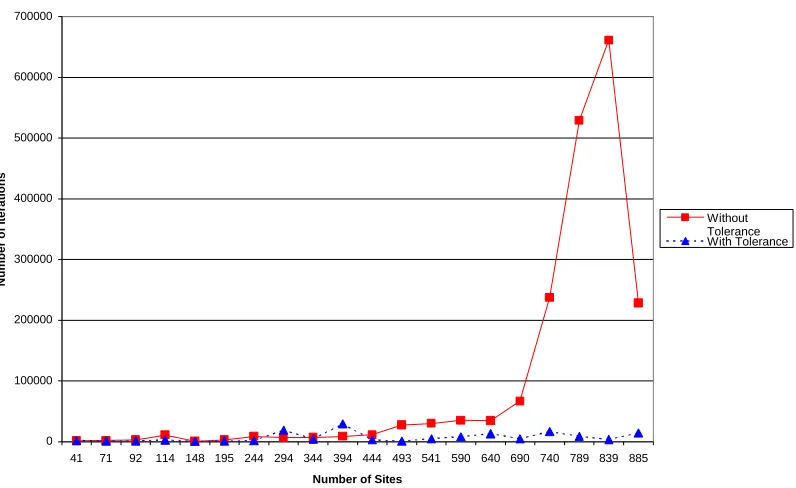
Table 2.2 and Figure 2.1 display the results for the comparison of the standard
branch-and-bound algorithm and the test of the .05% tolerance implementation. For these
tests, the objective function values were equal for all 20 tests between the use of
tolerance levels and without. The results of this test as the basis for deciding to use
the .05% tolerance when conducting further tests, especially for the 500 and 1000
mitigation target tests, which in pre-testing showed solution times of over three days
for a single test without the use of a tolerance. Identical acreage solutions were not
expected for the larger functional unit target levels (which require more acres in most
cases) however, since the tolerance is a percentage of the solution and not an absolute
Table 2.2: Number of Iterations Comparing Use of Tolerance for Wetlands Sorted by ID with a Target Mitigation of 100 FU
N u m b e r o f S i t e s W i t h o u t a T o l e r a n c e W i t h T o l e r a n c e
41 1279 1 9 8 3
71 1942 1 0 8 3
92 2791 1 1 0 1
114 1 1 1 8 1 2 7 8 5
148 566 1 8 9
195 3070 1 1 9 2
244 8700 1 7 0 6
294 6841 1 9 3 2 0
344 6826 4 2 2 8
394 8882 2 9 3 6 7
444 1 1 3 4 3 3 1 1 5
493 2 7 3 1 2 1 0 5 5
541 3 0 0 5 8 4 9 5 6
590 3 5 1 1 5 8 1 6 4
640 3 4 3 9 0 1 3 2 1 6
690 6 6 6 2 8 4 6 3 1
740 2 3 7 2 5 0 1 6 9 0 1
789 5 2 9 0 5 8 8 8 0 5
839 6 6 0 9 7 9 3 5 4 5
885 2 2 8 2 7 7 1 4 2 7 5
Figure 2.1: Comparison of Use of Tolerance with No Use of Tolerance 0 100000 200000 300000 400000 500000 600000 700000
41 71 92 114 148 195 244 294 344 394 444 493 541 590 640 690 740 789 839 885
Number of Sites
Number of Iterations
Tables 2.3 through 2.11 (following the DISCUSSION AND CONCLUSIONS)
contain the results for all the trials tested at the three functional unit levels. Two
important measures of performance are the time used to reach a solution and the
number of iterations. Figures 2.2 through 2.4 show a comparison of the number of
iterations required to reach a solution for the three trials. Those tests that did not reach
an optimal solution within 200 million iterations or where no feasible solution was
possible are not shown on the graphs to maintain readability. Figures 2.5 through 2.7
show the solution time for the trials. The solution times for the trials are somewhat
misleading because LINDO reported the computational time to trace through the
branches that met the tolerance requirements. Every branch is still visited on the tree
and the test to see if a branch is better than the current optimal solution is a
computation that takes time, but this time is not included in the output. For comparing
the trials, this method is consistent because it was applied to all tests, so the
comparisons are valid. However, it is not valid to assume that a model with 900
variables and a mitigation target of 1000 FU will take only 45 seconds. In actuality,
the model ran for approximately 23 hours before eliminating all possible other
solutions.
DISCUSSION AND CONCLUSIONS
The results from the trials confirm that with the given problem formulation and size,
one can optimize the selection of possible mitigation sites. All but 37 of the 180 tests
resulted in an optimal solution by LINDO. Fourteen of these were due to the imposed
or number of iterations among the three trials or the target functional unit values when
using a tolerance level. The erratic behavior of the graphs indicate there are numerous
factors affecting solution time, but that solutions are possible with properly
constructed models. The most important observation, however, was the nonfeasibility
of scenarios when the mitigation target levels were high and a small number of sites
were chosen based on their perimeter, which was sorted in ascending order. This
means that even if all the sites had been restored, their areas and ratings were not high
enough to meet the required mitigation target minimums. Therefore, for application
purposes, cases can be constructed to arrive at solutions for different mitigation
requirements and site selection criteria, as long as care is taken to avoid choosing sites
to include in the model based solely on their size, especially at the low end of the
spectrum. This can be extended to mean that if one is choosing possible sites to feed
into the model based on total site cost, selecting all the lowest sites could translate into
choosing the smallest sites. This depends, of course, on other factors that affect site
cost, but should still be a consideration.
The times associated with solving the models with larger numbers of sites can be
avoided by doing some logistical, political, and economical screening of sites to
include in the model (for example, selecting only sites that are potentially
purchasable). WetMOp used a sample watershed and assumed all sites were available
There is some overhead work that must be completed before the information could be
input into a model, but the majority of the tasks can be automated through scripts. The
limiting factor at this point is the availability of the NC-CREWS final ratings data
layers of the restoration functional assessment procedure. Because NC-CREWS
focuses on the coastal plain of North Carolina, WetMOp would have to be adapted to
manipulate the ratings from other assessment procedures. The model could also be
expanded to include more than three functions if the ratings were determined by a
consistent system. WetMOp also requires the input of functional units destroyed at
the impact site, which should be arrived at using the same “rating times acres” process
as used here to calculate restoration functional units.
Given the assumptions and limitations inherent in NC-CREWS and WetMOp, the
combination of the two systems provides a technique for mitigation planners to narrow
their field verification of possible sites. Future research and modification should focus
on converting the wetland ratings into mathematical formulas as well as the issue of
spatially dependent ratings when choosing sites. Larger processors and more efficient
algorithms also could have an effect on the solution time and intractability of integer
programming problems. It is important to choose a system and software package that
matches the requirements and size of the specific case.
Lessons from this model have yielded several important questions for further research:
What effect would non-estuarine wetlands have on the model since ratings may
calculate NC-CREWS ratings and run the model increase model reliability? How
sensitive is the optimization model to the input layers’ resolution and accuracy?
Would a network or some heuristic algorithm provide reliable answers in less time?
Answering these questions would provide a better model and hopefully a better tool
for selecting possible mitigation sites.
Table 2.3: Results of Tests for ID Sorted Trial with 100FU
Number of Sites Solution (acres) Iterations Time (seconds)
41 48.74 1983 0.88
71 34.15 1083 0.66
92 34.15 1101 0.99
114 33.87 2785 1.65
148 33.38 189 0.49
195 33.34 1192 1.43
244 33.34 1706 2.14
294 33.35 19320 18.56
344 33.34 4228 5.27
394 33.34 29367 35.70
444 33.34 3115 5.71
493 33.34 1055 2.80
541 33.34 4956 9.34
590 33.35 8164 16.48
640 33.34 13216 25.81
690 33.34 4631 11.31
740 33.35 16901 37.90
789 33.34 8805 26.31
839 33.34 3545 10.33
Table 2.4: Results of Tests for ID Sorted Trial with 500FU
Number of Sites Solution (acres) Iterations Time
41 246.25 253 0.27
71 205.74 1079 0.77
92 202.94 10240 5.27
114 184.58 6933 3.57
148 169.21 65159 31.03
195 166.83 8002 6.21
244 166.68 5652 5.11
294 166.69 132 0.82
344 166.69 4767 5.27
394 166.69 9531 12.08
444 166.68 7637 12.14
493 166.75 6777 12.47
541 166.70 7486 16.09
590 166.74 2321 5.22
640 166.67 7109 16.09
690 166.67 37007 92.33
740 166.75 38274 61.13
789 166.71 6693 16.86
839 166.70 6318 21.26
885 166.74 4495 16.59
Table 2.5: Results of Tests for ID Sorted Trial with 1000FU
Number of Sites Solution (acres) Iterations Time
41 NON-FEASIBLE **** ****
71 454.88 6475 2.03
92 452.82 5640 2.47
114 428.61 3935 1.98
148 386.73 4537 2.97
195 362.22 2000000 ****
244 356.35 11098 7.25
294 353.51 2000000 ****
344 352.74 29721 34.71
394 351.89 27879 34.22
444 350.68 569168 727.21
493 337.28 105.182 169.44
541 333.86 3638 8.24
590 333.48 8347 17.41
640 333.45 12010 26.25
690 333.36 14490 34.93
740 333.36 266 2.36
789 333.45 10435 36.85
839 333.35 16136 44.11
Table 2.6: Results of Tests for Perimeter Sorted Trial with 100FU
Number of Sites Solution (acres) Iterations Time
15 NON-FEASIBLE **** ****
33 NON-FEASIBLE **** ****
63 NON-FEASIBLE **** ****
112 75.37 621 0.66
161 55.98 292 0.88
209 40.72 37205 30.87
259 39.65 77366 50.97
306 39.64 1322426 1733.12
354 38.46 26744 41.52
402 38.08 18301 29.33
450 37.60 60856 118.58
500 35.90 200000000 ****
550 35.42 7034641 11700.26
599 33.88 630798 1062.64
646 33.64 19497 52.51
694 33.35 21647 60.53
742 33.35 5994 15.76
792 33.35 8714 23.18
842 33.34 12734 34.93
885 33.34 31724 95.73
Table 2.7: Results of Tests for Perimeter Sorted Trial with 500FU
Number of Sites Solution (acres) Iterations Time
15 NON-FEASIBLE **** ****
33 NON-FEASIBLE **** ****
63 NON-FEASIBLE **** ****
112 NON-FEASIBLE **** ****
161 NON-FEASIBLE **** ****
209 NON-FEASIBLE **** ****
259 NON-FEASIBLE **** ****
306 385.11 774 2.14
354 257.03 838 2.80
402 306.26 1467 2.75
450 240.40 1047 2.53
500 200.28 200000000 ****
550 195.43 200000000 ****
599 192.86 200000000 ****
646 191.42 200000000 ****
694 186.35 200000000 ****
742 172.91 200000000 ****
Table 2.8: Results of Tests for Perimeter Sorted Trial with 1000FU
Number of Sites Solution (acres) Iterations Time
15 NON-FEASIBLE **** ****
33 NON-FEASIBLE **** ****
63 NON-FEASIBLE **** ****
112 NON-FEASIBLE **** ****
161 NON-FEASIBLE **** ****
209 NON-FEASIBLE **** ****
259 NON-FEASIBLE **** ****
306 NON-FEASIBLE **** ****
354 NON-FEASIBLE **** ****
402 NON-FEASIBLE **** ****
450 740.39 690 3.46
500 654.93 2345 5.16
550 606.01 1090 5.11
599 529.97 4613 9.39
646 407.77 200000000 ****
694 390.77 200000000 ****
742 372.65 60544 139.07
792 365.74 34674 93.54
842 347.38 200000000 ****
885 333.46 30209 91.45
Table 2.9: Results of Tests for Random Sorted Trial with 100FU
Number of Sites Solution (acres) Iterations Time
44 37.01 1498 1.15
91 34.26 445 0.49
127 37.54 51597 48.39
178 33.55 47 0.55
217 33.49 1367 1.76
260 33.41 1591 1.98
314 33.36 9346 10.77
354 33.34 14315 15.05
406 33.35 4366 6.26
452 33.34 15743 26.91
492 33.34 11684 18.62
531 33.34 3112 5.88
582 33.34 11124 21.81
627 33.34 5632 13.02
655 33.34 16925 36.09
706 33.35 5949 17.08
754 33.34 11472 33.01
800 33.34 6284 17.58
849 33.34 13613 36.75
Table 2.10: Results of Tests for Random Sorted Trial with 500FU
Number of Sites Solution (acres) Iterations Time
44 3493.62 0 0.22
91 216.91 535 0.60
127 218.24 4134 1.81
178 191.08 52522 29.28
217 191.75 2000000 ****
260 166.71 671 1.59
314 166.76 6651 7.25
354 166.71 7516 10.66
406 170.40 102244 139.68
452 166.69 5058 10.88
492 166.67 150 1.48
531 166.70 1778 4.89
582 166.70 26578 59.98
627 166.70 3865 9.61
655 166.74 8287 20.38
706 166.68 4826 14.67
754 166.67 8435 20.43
800 166.68 33243 97.11
849 166.69 15271 42.90
885 166.74 4495 16.59
Table 2.11: Results of Tests for Random Sorted Trial with 1000FU
Number of Sites Solution (acres) Iterations Time
44 22467.75 3 0.33
91 1094.73 0 0.44
127 447.34 19298 6.26
178 432.40 1783 2.14
217 397.89 835560 559.31
260 358.42 2799 3.08
314 353.16 1061268 918.68
354 385.42 2000000 ****
406 370.39 82446 95.90
452 333.44 6411 11.37
492 333.38 4867 9.89
531 333.38 8551 15.76
582 333.36 17363 34.00
627 333.37 2383 6.81
655 333.41 2138 7.00
706 333.37 155 2.14
754 333.41 15731 36.47
Figure 2.2: Number of Sites vs. Iterations for ID Ordering
0 10000 20000 30000 40000 50000 60000 70000
41 71 92 114 148 195 244 294 344 394 444 493 541 590 640 690 740 789 839 885
Number of Sites
Number of Iterations
0 20000 40000 60000 80000 100000 120000 140000 160000
42 71 92 115 149 196 245 295 345 395 445 494 542 591 641 691 741 790 840 885
Number of Sites
Number of Iterations
100 FU 500 FU 1000 FU
Figure 2.4: Number of Sites vs. Iterations for Random Ordering
0 200000 400000 600000 800000 1000000 1200000
44 91 127 178 217 260 314 354 406 452 492 531 582 627 655 706 754 800 849 885 Number of Sites
Number of Iterations
Figure 2.5.— Number of Sites vs. Time for ID Ordering 0 . 0 0
2 0 . 0 0 4 0 . 0 0 6 0 . 0 0 8 0 . 0 0 1 0 0 . 0 0 1 2 0 . 0 0 1 4 0 . 0 0 1 6 0 . 0 0 1 8 0 . 0 0
4 1 7 1 9 2 1 1 4 1 4 8 1 9 5 2 4 4 2 9 4 3 4 4 3 9 4 4 4 4 4 9 3 5 4 1 5 9 0 6 4 0 6 9 0 7 4 0 7 8 9 8 3 9 8 8 5 N u m b e r o f S i t e s
Time (seconds)
Figure 2.6: Number of Sites vs. Time for Perimeter Ordering
0.00 2000.00 4000.00 6000.00 8000.00 10000.00 12000.00 14000.00
15 33 63
112 161 209 259 306 354 402 450 500 550 599 646 694 742 792 842 885
Number of sites
Time (seconds)
Figure 2.7: Number of Sites vs. Time for Random Ordering 0.00
100.00 200.00 300.00 400.00 500.00 600.00 700.00 800.00 900.00 1000.00
44 91 127 178 217 260 314 354 406 452 492 531 582 627 655 706 754 800 849 885
Number of Sites
Time (seconds)
REFERENCES
Bledsoe, Brian P. et al. 1997. A Geographic Information System for Targeting Wetland Restoration. North Carolina Department of Environment and Natural Resources. Raleigh, NC.
Haupt, Mac. 1997. NC DENR, Division of Coastal Management. Personal communication.
Logan, Bryan J. 1993. Digital Orthophotography Bolsters GIS Base for Wetlands Project. GIS World. June 1993. p.58-60.
Michelson, Daniel B. 1993. GIS Supports Wetlands Land Use Analysis. GIS World. 6:56-59.
Poiani, Karen A. and Bedford, Barbara L. 1995. GIS Based Nonpoint Source Pollution Modeling: Considerations for Wetlands. J of Soil and Water Conservation 5:613.
Schrage, L. Linear, Integer and quadratic programming with LINDO. 4th Edition. San Francisco: The Scientific Press, 1989.
Sutter, L.A. and Wuenscher, J.E. 1997. NC-CREWS: North Carolina Coastal Region Evaluation of Wetland Signifi cance, North Carolina Department of
Environmental Resources, Raleigh, NC.
Winston, Wayne L. Operation Research : Applications and Algorithms. Belmont: Duxbury Press, 1989.