Estimators For Generalized Linear Measurement Error Models With Interaction Terms

(1)

DAGALP, RUKIYE ESENER. Estimators For Generalized Linear Measurement Er-ror Models With Interaction Terms. (Under the direction of Professor Leonard A. Stefanski)

The primary objectives of this research are to develop and study estimators for generalized linear measurement error models when the mean function contains error-free predictors as well as predictors measured with error and interactions between error-free and error-prone predictors. Attention is restricted to generalized linear models in canonical form with independent additive Gaussian measurement error in the error-prone predictors.

Estimators appropriate for the functional (Fuller, 1987, Ch. 1) version of the mea-surement error model are derived and studied. The estimators are also appropriate in the structural version of the model and thus the methods developed in this research are functional in the sense of Carroll, Ruppert and Stefanski (1995, Ch. 6).

The primary approach to the development of estimators in this research is the

conditional-score method proposed by Stefanski and Carroll (1987) and described by Carroll et al. (1995, Ch. 6). Sufficient statistics for the unobserved predictors are obtained and the conditional distribution of the observed data given these sufficient statistics is derived. The latter admits unbiased score functions that are free of the nuisance parameters (the unobserved predictors) and are used to construct unbiased estimating equations for model parameters.

Estimators for the parameters of the model of interest are also derived using the corrected approach proposed by Nakamura (1990) and Stefanski (1989). These are also functional estimators in the sense of Carroll et al. (1995, Ch. 6) that are less dependent on the exponential-family model assumptions and thus provide a benchmark against which to compare the conditional-score estimators.

(2)

by

RUKIYE E. DAGALP

A dissertation submitted in partial satisfaction of the requirements for the degree of

Doctor of Philosophy

in STATISTICS

in the

GRADUATE SCHOOL at

NC STATE UNIVERSITY 2001

Professor Leonard A. Stefanski Professor William H. Swallow Chair of Advisory Committee

(3)

(4)

Biography

(5)

Acknowledgements

My sincere gratitude is given to those who supported me during my academic career. Without your help, friendship and advice I would not have succeeded. I would especially like to thank the following individuals:

• Dr. Leonard A. Stefanski, my advisor, mentor and friend. I cannot thank you enough for your patience, insight, encouragement, wonderful proofreading throughout this dissertation, and for introducing me to the area of measurement error models. It has been a great pleasure working with you.

• Drs. William H. Swallow, John F. Monahan, and Dennis D. Boos. Thank you for serving on my committee and providing useful comments on my dissertation. • Dr. Sastry Pantula, NCSU Director of Graduate Programs. Thank you for all

your support, help and advice.

• Dr. James Stapleton, MSU Director of Graduate Programs. Thank you for your encouragement and belief in me to complete the Ph.D. program.

• Drs. Bibhuti B. Bhattacharyya, Anastasios Tsiatis, Marie Davidian, Fikri Oz-turk, and Hamza Gamgam who have been the most influential instructors in my academic career.

• Dr. Harvey J. Charlton, NCSU Department of Mathematics. Thank you for your financial support and friendship throughout my study.

• Terry Byron, NCSU Department of Statistics Systems Administrator. Thank you for your help with my computer questions and for always being willing to lend a helping hand.

(6)

• Kath & Dave Williams, thank you for taking care of me during my pregnancy, for your friendship, and your delicious dinners.

• Fellow graduate students at NCSU: Josh Tebbs, Steve Novick, Jared Lunceford, Jimmy Doi, Ann Oberg, Elizabeth Johnson. Thanks to each of you for your kindness, support and friendship. A especial thanks to Jared for being the SAS/IML manual for me, and Jimmy for proofreading my thesis.

• Janice Gaddy, Sharon Patton, especially Brenda Currin. Thank you all for your sweet kindness, willingness to assist and friendship.

• Hatice & Adem C. Esener, my parents, who continually encouraged me through-out my Ph.D. program. Thank you for your never ending love and support. • Finally, to my husband Volkan and my son Alper. I cannot thank you enough for

(7)

List of Tables

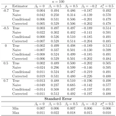
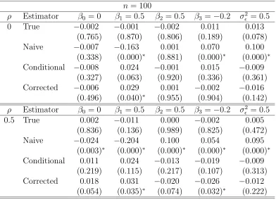
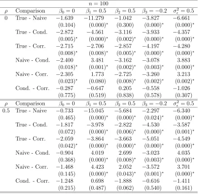
3.1 Simulation study results for the true, naive, conditional-score and corrected-score estimators for the normal linear model with parameters Θ= (β₀, β₁, β₂, β₃, σ_²2)T = (0,0.5,0.5,−0.2,0.5)T and measurement er-ror variance σ_U2 = 0.5. Table entries are means of 100 Monte Carlo runs for sample size n = 100. The entries at the bottom of the table are minimum and maximum values of standard errors for the parameters. 40 3.2 Simulation study results for the true, naive, conditional-score and

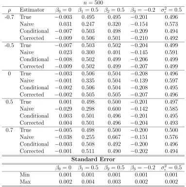
corrected-score estimators for the normal linear model with parameters Θ= (β₀, β₁, β₂, β₃, σ_²2)T = (0,0.5,0.5,−0.2,0.5)T and measurement er-ror variance σ_U2 = 0.5. Table entries are means of 100 Monte Carlo runs for sample size n = 500. The entries at the bottom of the table are minimum and maximum values of standard errors for the parameters. 41 3.3 Simulation study results to analyze biases of the true, naive,

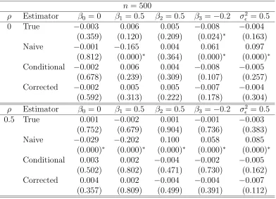
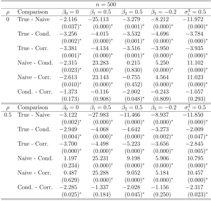
conditional-score and corrected-conditional-score estimators for the normal linear model with parameters Θ = (β₀, β₁, β₂, β₃, σ_²2)T = (0,0.5,0.5,−0.2,0.5)T, mea-surement error variance σ_U2 = 0.5 and n = 100. Table entries are mean biases and p-values of t−tests for no-bias (in parentheses) for 100 Monte Carlo runs. . . 42 3.4 Simulation study results to analyze biases of the true, naive,

conditional-score and corrected-conditional-score estimators for the normal linear model with parameters Θ = (β₀, β₁, β₂, β₃, σ_²2)T = (0,0.5,0.5,−0.2,0.5)T, mea-surement error variance σ_U2 = 0.5 and n = 500. Table entries are mean biases and p-values of t−tests for no-bias (in parentheses) for 100 Monte Carlo runs. . . 43 3.5 Simulation study results to compare differences in biases of the true,

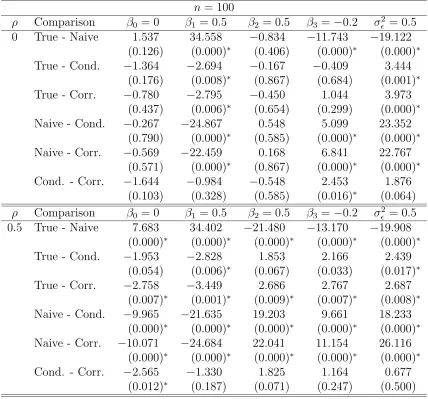
naive, conditional-score and corrected-score estimators for the normal

linear model with parametersΘ= (β₀, β₁, β₂, β₃, σ_²2)T = (0,0.5,0.5,−0.2,0.5)T, measurement error variance σ_U2 = 0.5 and n = 100. Table entries are

(10)

3.6 Simulation study results to compare differences in biases of the true, naive, conditional-score and corrected-score estimators for the normal

linear model with parametersΘ= (β₀, β₁, β₂, β₃, σ_²2)T _{= (0,}_0.5,_0.5,₋_0.2,_0.5)T_,

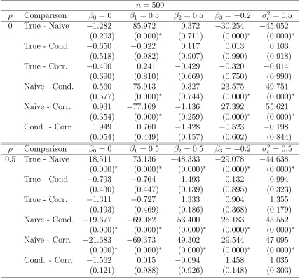
measurement error variance σ_U2 = 0.5 and n = 500. Table entries are paired t−test statistics and p−values (in parentheses) for 100 Monte Carlo runs. . . 45 3.7 Simulation study results to compare mean squared errors of the true,

measurement error variance σ_U2 = 0.5 and n = 500. Table entries are paired t−test statistics and p−values (in parentheses) for 100 Monte Carlo runs. . . 47 3.9 Simulation study results to estimate the Monte Carlo, sandwich and

model-based variances for the true, naive, conditional-score and corrected-score estimators for the normal linear model with parameters Θ = (β₀, β₁, β₂, β₃, σ_²2)T = (0,0.5,0.5,−0.2,0.5)T, measurement error vari-ance σ2_U = 0, the correlation of X₁ and X₂, ρ= 0, and n= 100. Table entries (in last two columns) are the means and standard errors (in parentheses) of ratios of the mean of sandwich variance estimates to the mean of model-based variance estimates from five replicates each from 100 Monte Carlo runs. . . 49 3.10 Simulation study results to estimate the Monte Carlo, sandwich and

(11)

3.11 Simulation study results to estimate the Monte Carlo, sandwich and model-based variances for the true, naive, conditional-score and corrected-score estimators for the normal linear model with parameters Θ = (β₀, β₁, β₂, β₃, σ_²2)T = (0,0.5,0.5,−0.2,0.5)T, measurement error vari-ance σ2_U = 0.5, the correlation of X₁ and X₂, ρ = 0.5, and n = 100. Table entries (in last two columns) are the means and standard errors (in parentheses) of ratios of the mean of sandwich variance estimates to the mean of model-based variance estimates from five replicates each from 100 Monte Carlo runs. . . 51 3.12 Simulation study results to estimate the Monte Carlo, sandwich and

model-based variances for the true, naive, conditional-score and corrected-score estimators for the normal linear model with parameters Θ = (β₀, β₁, β₂, β₃, σ_²2)T = (0,0.5,0.5,−0.2,0.5)T, measurement error vari-ance σ2_U = 0.5, the correlation of X₁ and X₂, ρ = 0.5, and n = 500. Table entries (in last two columns) are the means and standard errors (in parentheses) of ratios of the mean of sandwich variance estimates to the mean of model-based variance estimates from five replicates each from 100 Monte Carlo runs. . . 52 3.13 The 95% confidence intervals for relative effiencies of the

conditional-score and the corrected-conditional-score estimators when (X₁, X₂)∼MVN(0,0, σ2_X

1, σX22, ρ)

under the measurement error varianceσ_U2 = 0.5, and the true parame-ters Θ= (β₀, β₁, β₂, β₃, σ2_²)T = (0,0.5,0.5,−0.2,0.5)T. The results are 102∗95% CI of the mean of four REs of 100,000 Monte Carlo runs. . 55 3.14 The 95% confidence intervals for relative effiencies of the conditional

score and the corrected-score estimators whenX₂ is Binomial(1,π) and X1|X₂ is Normal with mean µ_X₂ = µ₀I{X₂ = 0} +µ₁I{X₂ = 1} and σ_X2₂ = σ₀2I{X₂ = 0}+σ₁2I{X₂ = 1} under measurement error variance σ2_U = 0.5 and the true parameters Θ= (β₀, β₁, β₂, β₃, σ2_²)T = (0,0.5,0.5,−0.2,0.5)T_{. The results are 10}2 _∗_{95% CI of the mean of}

four REs of 100,000 Monte Carlo runs where µ₀ = 0 and µ₁ = 1. . . . 56 4.1 Simulation study results for the true, naive, conditional-score and

corrected-score estimators for the logistic regression model with pa-rameters Θ= (β₀, β₁, β₂, β₃,)T _{= (0,}_0.5,_0.5,₋_0.2)T_{, measurement}

(12)

4.2 Simulation study results for the true, naive, conditional-score and corrected-score estimators for the logistic regression model with pa-rameters Θ= (β₀, β₁, β₂, β₃,)T _{= (0,}_0.5,_0.5,₋_0.2)T_{, measurement}

er-ror variance σ2_U = 0.5, and sample size n = 1000. Table entries are means of 100 Monte Carlo runs. The entries at the bottom of the table are minimum and maximum values of standard errors for the parameters. 72 4.3 Simulation study results to analyze biases of the true, naive,

conditional-score and corrected-conditional-score estimators for the logistic regression model with parameters Θ = (β₀, β₁, β₂, β₃)T _{= (0,}_0.5,_0.5,₋_0.2)T_,

measure-ment error variance σ2_U = 0.5 andn = 500. Table entries are mean bi-ases and p-values oft−tests for no-bias (in parentheses) for 100 Monte Carlo runs. . . 73 4.4 Simulation study results to analyze biases of the true, naive,

conditional-score and corrected-conditional-score estimators for the logistic regression model with parameters Θ = (β₀, β₁, β₂, β₃)T _{= (0,}_0.5,_0.5,₋_0.2)T_,

measure-ment error varianceσ2_U = 0.5 andn= 1000. Table entries are mean bi-ases and p-values oft−tests for no-bias (in parentheses) for 100 Monte Carlo runs. . . 74 4.5 Simulation study results to compare differences in biases of the true,

naive, conditional-score and corrected-score estimators for the logistic regression model with parametersΘ= (β₀, β₁, β₂, β₃)T _{= (0,}_0.5,_0.5,₋_0.2)T_,

measurement error variance σ_U2 = 0.5 and n = 500. Table entries are paired t−test statistics and p−values (in parentheses) for 100 Monte Carlo runs. . . 75 4.6 Simulation study results to compare differences in biases of the true,

measurement error variance σ2_U = 0.5 and n= 1000. Table entries are paired t−test statistics and p−values (in parentheses) for 100 Monte Carlo runs. . . 76 4.7 Simulation study results to compare mean squared errors of the true,

(13)

4.9 Simulation study results to estimate the Monte Carlo, sandwich and model-based variances for the true, naive, conditional-score and corrected-score estimators for the logistic regression model with parametersΘ= (β₀, β₁, β₂, β₃)T = (0,0.5,0.5,−0.2)T, measurement error varianceσ2_U = 0.5, the correlation of X₁ and X₂, ρ = 0, and n = 500. Table entries (in last two columns) are ratios of the mean of sandwich variance esti-mates to the mean of model-based variance estiesti-mates from 100 Monte Carlo runs. These ratios have standard error approximate equal to 0.14. 80 4.10 Simulation study results to estimate the Monte Carlo, sandwich and

model-based variances for the true, naive, conditional-score and corrected-score estimators for the logistic regression model with parametersΘ= (β₀, β₁, β₂, β₃)T _{= (0,}_0.5,_0.5,₋_0.2)T_{, measurement error variance}_σ2

U =

0.5, the correlation of X₁ and X₂, ρ= 0, and n = 1000. Table entries (in last two columns) are ratios of the mean of sandwich variance esti-mates to the mean of model-based variance estiesti-mates from 100 Monte Carlo runs. These ratios have standard error approximate equal to 0.14. 81 4.11 Simulation study results to estimate the Monte Carlo, sandwich and

model-based variances for the true, naive, conditional-score and corrected-score estimators for the logistic regression model with parametersΘ= (β₀, β₁, β₂, β₃)T _{= (0,}_0.5,_0.5,₋_0.2)T_{, measurement error variance}_σ2

U =

0.5, the correlation of X₁ and X₂, ρ= 0.5, and n= 500. Table entries (in last two columns) are ratios of the mean of sandwich variance esti-mates to the mean of model-based variance estiesti-mates from 100 Monte Carlo runs. These ratios have standard error approximate equal to 0.14. 82 4.12 Simulation study results to estimate the Monte Carlo, sandwich and

model-based variances for the true, naive, conditional-score and corrected-score estimators for the logistic regression model with parametersΘ= (β₀, β₁, β₂, β₃)T = (0,0.5,0.5,−0.2)T, measurement error varianceσ2_U = 0.5, the correlation ofX₁ andX₂,ρ= 0.5, andn= 1000. Table entries (in last two columns) are ratios of the mean of sandwich variance esti-mates to the mean of model-based variance estiesti-mates from 100 Monte Carlo runs. These ratios have standard error approximate equal to 0.14. 83 4.13 Framingham Heart study to estimate for naive, conditional-score and

Monte-Carlo corrected-score estimators with sample size, n = 1615, and their standard errors. ln(Cholest2) is the ln transformation of the single measurement of serum cholesterol at Exam 2 and the observed covariate is age. . . 85 4.14 Framingham Heart study to estimate for naive, conditional-score and

(14)

4.15 Framingham Heart study to estimate for naive, conditional-score and Monte-Carlo corrected-score estimators with sample size, n = 1615, and their standard errors. ln(SBP2−50) is ln transformation of (SBP2 − 50) and the observed covariate is smoke. . . 89 4.16 Framingham Heart study to estimate for naive, conditional-score and

(15)

List of Figures

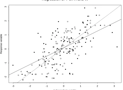
1.1 Illustration of the classical measurement error model in simple linear regression. The steeper line and the empty circles are the least squares fit and the plot of the true (Y, X) data, respectively. The attenuated line and the filled circles are the least squares fit and the plot of the observed (Y, W) data, respectively. For these data σ_X2 = σ2_U = 1, (α, β) = (0,1) andσ_²2 = 0.5. . . 5 1.2 Illustration of the classical measurement error model in logistic

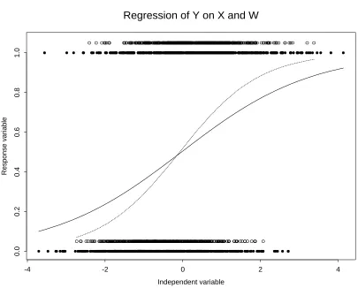
regres-sion. The empty circles are the true (X, Y) data and the filled circles are the observed (W, Y) data. The dotted and solid (attenuated) curves are (X, F(αb_{T rue}+βb_{T rue}X)) and (W, F(αb_{N aive}+βb_{N aive}W)), respectively. For these dataσ_X2 =σ_U2 = 1 and (α, β) = (0,1). . . 7 4.1 The regression fits of CHD on single measurement of ln(Cholest2)

and Age for Naive, Conditional-score and Monte-Carlo Corrected-score methods. . . 86 4.2 The regression fits of CHD on average measurements of ln(Cholest) Age

for Naive, Conditional-score and Monte-Carlo Corrected-score methods. 88 4.3 The regression fits of CHD on measurements of ln(SBP2 - 50) and

Non-Smoke for Naive, Conditional-score and Monte-Carlo Corrected-score methods. . . 89 4.4 The regression fits of CHD on measurements of ln(SBP2 - 50) and

Smoke for Naive, Conditional-score and Monte-Carlo Corrected-score methods. . . 90 4.5 The regression fits of CHD on average measurements of ln(SBP) and

Non-Smoke for Naive, Conditional-score and Monte-Carlo Corrected-score methods. . . 92 4.6 The regression fits of CHD on average measurements of ln(SBP) and

(16)

Chapter 1 Introduction

1.1 Measurement Error Models

Regression analysis is a statistical methodology for studying the relationship be-tween two or more quantitative variables so that one variable can be explained from the other variables. The response variableY is a dependent variable whose variation can be explained by an explanatory variable or independent variable X which must be observable in traditional regression analysis. Sometimes the explanatory variable X cannot be observed, either because it is too expensive, unavailable, or mismea-sured. In this situation, a substitute variable W is observed instead of X, that is W = X +U, where U is measurement error. When the conditional distribution of Y given (X, W) is the same as the conditional distribution of Y given X, that is f_Y_|_X,W =f_Y_|_X, andW =X+U,W is said to be asurrogate forX. The substitution ofW for X creates problems in the analysis of the data, generally referred to as mea-surement error problems. The statistical models used to analyze such data are called

(17)

The purpose of regression analysis is to model the dependence of the conditional mean of Y given X mathematically via a regression function f, namely

E(Y|X) =f(X;θ), (1.1)

where θ is an unknown parameter to be estimated. In a measurement error problem there are two problems in modeling the regression of Y on X. One is with the unknown parameter θ and the other is that {(Y_j, W_j), j = 1,2, . . . , n} are observed rather than {(Y_j, X_j), j = 1,2, . . . , n}.

Often the relationship between X and W can be explained by a classical additive measurement error model

W =X+U, (1.2)

where U is a normally distributed measurement error with zero mean and variance σ_U2 and is independent of Y and X. The unobserved variable X is sometimes called the true regressor and can be either fixed or random. According to the characteristic of X, the measurement error models are called either functional models with fixedX orstructural models with random X (Fuller, 1987).

There are two important types of measurement error models depending on the distribution of X orW. The first one, the so-called classical error model, is given in (1.2). In this case W is an unbiased measure of X in the sense that E(W|X) = X and W is a surrogate forX in the sense that the conditional distribution of Y given X andW is the same as the conditional distribution ofY givenX. The latter implies that U is independent of Y and the residual isY −E(Y|X).

When E(X|W) = W, the measurement error model is called the Berkson error model, andW is called anunbiased Berkson predictor of X. That is,X varies around W and the measurement error model is

X =W +U, (1.3)

(18)

Y −E(Y|X) are uncorrelated and the residual is uncorrelated withX. For both mea-surement error models, the meamea-surement error U could be homoscedastic (constant variance) or heteroscedastic. In this thesis, we assume the classical measurement error model with known measurement error variance andW is a surrogate for X.

Parameter estimators obtained by ignoring the error in W as measurement of X and fitting the regression model to the observed data, are referred to asnaive estima-tors. These are generally biased and inconsistent estimators of the true parameters in the regression of Y given X. In simple linear regression, and in generalized linear regression models more generally, it is often the case that naive estimators of the regression coefficient of variables measured with error are biased toward zero. This type of bias called attenuation. It is well known and understood in the context of simple linear regression.

In simple linear regression, the amount of attenuation is called the reliability ra-tio (Fuller, 1987) and is commonly denoted by λ. The reliability ratio provides an approximate measure of attenuation in generalized linear measurement error models more generally and it will be referenced throughout this thesis in connection with both linear and nonlinear measurement error models.

We complete this subsection with an illustration and further discussion of mea-surement error-induced bias in the context of two simple regression models.

1.1.1 Simple Linear Regression

Consider the classical linear regression model with one independent variable that is unobservable

Y =α+βX +², with the classical measurement error model

(19)

where X is the true predictor, measured with error, U is the measurement error and W is a surrogate forX. Suppose{², U, X}is an independent triplet with distribution

      ² U X      ∼N

                 0 0 µ_X      ,      

σ_²2 0 0 0 σ_U2 0 0 0 σ_X2

                 .

Consistent estimating equations of intercept and slope based on the error-free data, given by the likelihood function, are

n

X

j=1

(Y_j −α−βX_j)

  1 X_j  =   0 0 

. (1.4)

The equations in (1.4) yield the ordinary least squares estimate of slope given by

b

β_{T rue}= SXY S_XX =

(n−1)−1Pn_j₌₁(Y_j−Y)X_j (n−1)−1Pn_j₌₁(X_j −X)2 .

Substituting W for X in (1.4) yields the so-called naive slope estimator,

b

β_{N aive} = SW Y S_{W W} =

(n−1)−1Pn_j₌₁(Y_j−Y)W_j (n−1)−1Pn_j₌₁(W_j −W)2 = (n−1)

−1Pn

j=1(Yj−Y)(Xj +Uj)

(n−1)−1Pn_j₌₁(X_j+U_j−X−U)2 = SY X+SY U

S_XX+ 2S_XU +S_{U U},

where S_XX is the sample variance of X₁, . . . , X_n, S_{U U} is the sample variance of U₁, . . . , U_n, S_XU is the sample covariance of (X_j, U_j), j = 1, . . . , n, and other com-ponents are defined similarly. By the Law of Large Numbers, both S_{Y U} and S_XU converge to zero, S_XX−→P σ_X2, and S_{U U}−→P σ_U2, as n → ∞. Thus,

b

β_{N aive}−→P λβ, as n → ∞

(20)

Independent variable

Response variable

-3 -2 -1 0 1 2 3

-2 -1 0 1 2 3

Regression of Y on X and W

Figure 1.1: Illustration of the classical measurement error model in simple linear regression. The steeper line and the empty circles are the least squares fit and the plot of the true (Y, X) data, respectively. The attenuated line and the filled circles are the least squares fit and the plot of the observed (Y, W) data, respectively. For these data σ_X2 =σ2_U = 1, (α, β) = (0,1) and σ2_² = 0.5.

Figure 1.1 illustrates the attenuation induced by measurement error. For this illustration, data were generated with α = 0, β = 1 and a sample size of 100. The true covariate X, the regression experimental error ², and the measurement error U were generated from the normal distribution

      X U ²      ∼N

                 0 0 0      ,      

1 0 0 0 1 0 0 0 0.5

                 .

(21)

1.1.2 Simple Logistic Regression

Consider the logistic regression model with mean function E(Y|X) = Pr(Y = 1|X) = F(α+βX),

whereF(t) ={1 +e−t}−1 _{is the logistic function with the classical measurement error}

model

W =X+U,

whereU is N(0, σ_U2), independent of all other variables, and the conditional distribu-tion ofW givenX is N(X, σ_U2). Defineθ = (α, β)T_{. Consistent estimating equations}

for intercept and slope based on the error-free data, given by the likelihood function, are

n

X

j=1

{Y_j −F(α+βX_j)}

  1 X_j   ₌   0 0 

_. _(1.5)

The estimator solving (1.5) will be called the true estimator and denoted by θb_{T rue}. When the measurement error is ignored and W is substituted for X, the resulting estimating equations for intercept and slope are

n

X

j=1

{Y_j −F(α+βW_j)}

  1 W_j   =   0 0 

. (1.6)

The estimator solving (1.6) will be called the naive estimator and designated by

b

θ_{N aive}.

Logistic regression estimators are nonlinear and have no closed-form expressions. Thus it is not possible to derive a mathematical expression for measurement error-induced bias in logistic regression. However, attenuation is easily demonstrated using simulated data sets. Figure 1.2 illustrates the attenuation induced by measurement error. For this graph, data were generated withα = 0 andβ = 1 and the sample size of 1000. The true covariateX and the measurement error U were generated from the standard bivariate normal distribution.

  X

U

 _∼N

     0 0  ,   1 0

(22)

Regression of Y on X and W

Independent variable

Response variable

-4 -2 0 2 4

0.0

0.2

0.4

0.6

0.8

1.0

Figure 1.2: Illustration of the classical measurement error model in logistic regression. The empty circles are the true (X, Y) data and the filled circles are the observed (W, Y) data. The dotted and solid (attenuated) curves are (X, F(αb_{T rue}+βb_{T rue}X)) and (W, F(αb_{N aive}+βb_{N aive}W)), respectively. For these dataσ_X2 =σ_U2 = 1 and (α, β) = (0,1).

(23)

1.2 Statistical Inference in the Presence of

Mea-surement Error

The study of measurement error problems in regression modeling is an active area of statistical research. The most comprehensive discussion of methods for linear measurement error models is the book by Fuller (1987). Statistical methods for nonlinear measurement error models are described in the book by Carroll, Ruppert and Stefanski (1995).

In this thesis two methods appropriate for functional measurement error models will be developed for a particular class of generalized linear measurement error models with interaction terms. The two methods, one based on conditional-scores, the other based on corrected-scores, are discussed in the following sections.

1.2.1 The Conditional-Score

In this section, the conditional-score estimators of Stefanski and Carroll (1987) are described for an important class of generalized linear measurement error mod-els. When measurement error is present, the naive estimating equations produce an estimator which is biased and inconsistent due to measurement error. The idea is to obtain an unbiased estimating equation for θ, that does not depend on the nuisance parameters and produces an asymptotically unbiased estimator. The con-ditional distribution of the response variable Y given a statistic that is sufficient for the unobserved covariate X, does not depend on X. Thus, it is possible to derive unbiased estimating equations for θ that do not depend on X. Conditional-scores are derived under the assumption of normally distributed measurement errors (the classical model) with known error variance.

(24)

for response variable Y, given explanatory variables X = (X₁,X₂)T, have density f_Y_|_X(y|x;θ) = exp

(

yη−b(η)

φ +c(y, φ)

)

, (1.7)

where η=α+βT₁x₁+βT₂x₂ is called the natural parameter and θ = (α,βT₁,βT₂, φ)T

is the unknown parameter. The mean and variance of Y are b0(η) and φb00(η), where b0 and b00 are the first and second derivatives of b(η) with respect to η. The class of models includes:

• Linear regression:

E(Y|X) = η, Var(Y|X) = φ, b(η) = η 2

2, c(y, φ) = − y2

2φ −log( √

2πφ) • Logistic regression:

E(Y|X) = H(η), Var(Y|X) =H0(η),φ = 1, b(η) = −log{1−H(η)}, c(y, φ) = 0, whereH(t) ={1 +e−t_}−1

• Poisson log-linear regression:

E(Y|X) = Var(Y|X) = eη, φ = 1, b(η) = eη, c(y, φ) =−log(y!) • Gamma inverse regression:

E(Y|X) =−1

η, Var(Y|X) =− φ

η, b(η) =−log(−η), c(y, φ) = log(y/φ)

φ −log{yΓ(1/φ)}.

If both X₁ and X₂ were observed, the usual estimating equations forΘ have the form

n

X

j=1

{Y_j −b0(η_j)}

      1

X1j

X2j

      =       0 0 0      , and n X j=1

(µ_n₋_p

n

¶

φ− {Yj −b 0_(η

j)}2

b00(η_j)

)

= 0,

(25)

X1 is considered as an unknown parameter and α,β1,β2 and φ as fixed, then the statistic∆=W+YΩ_Uβ₁/φ is complete and sufficient for X₁ (Stefanski & Carroll, 1987). Now, the conditional distribution of Y given ∆ and X₂ is free of X₁, so the unbiased estimating equations for Θ are independent ofX₁. It is possible to derive the mean and variance ofY given∆andX₂ by the density ofY|∆,X₂ which is also a canonical generalized linear model in the same form as (1.7). The conditional-score function is derived in general for the exponential family in canonical form and is given in detail in Chapters 2, 3 and 4.

1.2.2 The Corrected-Score

The corrected-score method is a technique for eliminating asymptotic bias caused by measurement error by using unbiased estimating equations for the parameter of interest (Stefanski, 1989, and Nakamura, 1990). It assumes the existence of an unbi-ased score for the true data that is, when both X₁ and X₂ are error-free predictors, one would estimate the unknown parameter Θ in the absence of measurement error as the solutions of the equations

n

X

j=1

ψ(Y_j,X₁_j,X₂_j;cΘ) =0, (1.8)

where ψ is a likelihood score function from the model for the true data. The data {Y_j,X₁_j,X₂_j}n

j=1 are assumed to be independent random vectors such that

E{ψ(Y,X₁,X₂;Θ)}=0. (1.9) Estimators defined in (1.8) are called M-estimators.

When measurement error is normally distributed with known variance Ω_U, a con-sistent estimator of the parameter of interest in nonlinear measurement error models is difficult to obtain (Stefanski, 1989) in general. However, suppose that there exists some score function, ψ∗(Y,W,X₂;Θ) of the observed data having the property

(26)

for all Y,X₁,X₂ and Θ. It follows that

E{ψ∗(Y,W,X₂;Θ)} = E{E{ψ∗(Y,W,X₂;Θ)|Y,X₁,X2}} = E{ψ(Y,X₁,X₂;Θ)}=0,

so thatψ∗(·,·,·,·) is a Fisher-consistent score function (Carroll, Ruppert & Stefanski, 1995). The M-estimator Θ∗ based on the observed data is defined as the solution to

n

X

j=1

ψ∗_(Y

j,Wj,X2j;Θ∗) =0, (1.11)

and is then generally consistent forΘ. A score functionψ∗(·,·,·,·) satisfying (1.10) is called acorrected-score function and the parameter estimator,Θ∗ that satisfies (1.11) is called a corrected-score estimator.

The problem is that the corrected-score function satisfying (1.10) does not al-ways exist, and when it exists, it is not easy to find. For some common models, corrected-score functions have been studied and derived in detail by Stefanski (1989) and Nakamura (1990). Theorem 1 in Stefanski (1989) provides a means of deter-mining corrected-score functions for a large class of models. Let Z be independent standard normal errors independent of all other variables, and let i=√−1. If f(·) is an entire function of the complex variable and the indicated expectations exist, then Enf(W +iΩ1_U/2Z)|Xo=f(X). (1.12) Examples of how to obtain an unbiased corrected-score function using this result are given in Stefanski (1989).

Application to the measurement error models problems results in the corrected-score

ψ∗_(Y,_W_,_X

2;Θ) = E

n

ψ(Y,W +iΩ1_U/2Z,X₂;Θ)|Y,W,X₂o. (1.13)

(27)

1.3 Outline of Thesis

This thesis will focus on the classical measurement error model in (1.2) where the measurement error U is homoscedastic and normally distributed. The primary objective of this thesis is to study the effect of measurement error and to eliminate asymptotic bias when there exists an interaction between observed and unobserved true covariates of the form

E(Y|X₁,X₂) =b0(β₀+βT₁X₁+βT₂X₂ +XT₁β₃X₂),

for canonical generalized linear models, where β₀,β₁,β₂ and β₃ are unknown regres-sion coefficients. For eliminating bias due to measurement error, the conditional-score method (Stefanski & Carroll, 1987) and the corrected-score method (Stefanski, 1989, Nakamura, 1990) are studied for the regression models with interaction terms.

(28)

Chapter 2 Generalized Linear Measurement

Error Models and

Conditional-Scores

The statistical models studied in this dissertation have the exponential family form given in McCullagh & Nelder (1989, Chap. 2). Given a covariate p×1 vector

X =x, the response variable Y has density function as a generalized linear model in canonical form

f_Y_|_X(y|x,Θ) = exp

(

yη−b(η)

a(φ) +c(y, φ)

)

, (2.1)

with respect to aσ-finite measurem(·). Generalized linear models of this form include normal, Poisson, gamma, inverse Gaussian and logistic models. The normal linear and the logistic regression models are discussed in Chapters 3 and 4, respectively. In (2.1) functions a(·), b(·) and c(·,·) are known and η is called the natural parameter

and is a function of the predictor and unknown regression parameters. This thesis focuses exclusively on the case in which η has the form

η =η(X₁,X₂;Θ) =β₀+βT₁X₁+βT₂X₂+XT₁β₃X₂, (2.2) where Θ = (β₀,βT₁,βT₂,βT₃₁,βT₃₂, . . . ,βT₃_p₂, φ)T _{is a (p}

(29)

β₃_k is a p₁ ×1 vector, k = 1, . . . , p₂. The predictor X₁ is an unobservable p₁ ×1 vector, butX₂ is an observablep₂×1 vector withX = (X₁,X₂)T_{. The novel feature}

of this model is the interaction term between the predictor measured with error X₁ and the error-free predictor X₂. The mean and variance ofY given X are b0(η) and φb00(η), where b0 and b00 are the first and second derivatives of b(η) with respect to η, respectively. The measurement of the error-prone predictor is denoted by W and is assumed to satisfy

W =X₁+U, (2.3)

where the measurement errorU is distributed as a normal random vector with mean zero and covariance matrix Ω_U, independent of X₁,X₂ and Y. In this case the density of W given X₁ =x₁ is

f_W_|_X₁(w|x₁,Ω_U) = (2π)−p21 |_Ω_U |−12 _exp

½

−1

2(w−x1)

T_Ω−1

U (w−x1)

¾

. (2.4) The models in (2.1) and (2.4) together define a generalized linear measurement error model with interaction terms.

Combining (2.1) and (2.4) results in the joint density of (Y,W) given the unob-served predictor x₁ and observed predictorx₂,

f_Y,W_|_X₁_,X₂(y,w|x₁,x₂;Θ) =f_Y_|_X₁_,X₂(y|x₁,x₂;Θ)f_W_|_X₁_,X₂(w|x₁,x₂). (2.5) Functional maximum likelihood estimation maximizes the likelihood as a function of Θ and the unobserved predictors x₁₁, . . . ,x₁_n, i.e.,

L(Θ;x₁₁, . . . ,x₁_n|(Y₁,W₁), . . . ,(Y_n,W_n)) =

n

X

j=1

log{f_Y,W_|_X₁_,X₂(Y_j,W_j|x₁_j,x₂_j;Θ)}(2.6).

(30)

approach is adapted here and used to derive conditional estimating equations for generalized linear models with interaction terms.

Consider the joint density in (2.5). Define Ωas Ω= ΩU

a(φ). (2.7)

Note that f_W_|_X₁(w|x₁) = f_W_|_X₁_,X₂(w|x₁,x₂). Under (2.1), (2.4) and (2.7), the joint density of (Y,W) givenX₁ =x₁ and X₂ =x₂ is

f_Y,W_|_X₁_,X₂(y,w|x₁,x₂;Θ) = f_Y_|_X₁_,X₂(y|x₁,x₂;Θ)f_W_|_X₁(w|x₁) (2.8)

= exp

(

yη−b(η)

a(φ) +c(y, φ)

)

(2π)−p21 |Ω_U |−12 exp

½

−1

2(w−x1)

T_Ω−1

U (w−x1)

¾

= exp

(

yβ₀+yxT

1(β1+β3x2) +yxT2β2−b(η)

a(φ) +c(y, φ)− 1 2w

T_Ω−1 U w

+xT₁Ω−1_U w− 1 2x

T

1Ω−1U x1−

1

2log [(2π)

p1 _|_Ω

U |]

)

= exp

(

xT

1Ω−1U

"

yΩ_U(β₁+β₃x₂) a(φ) +w

#

+y(β0+x

T

2β2)−b(η)

a(φ) +c(y, φ) −1

2(w

T_Ω−1

U w+xT1Ω−1U x1)−

1

2log [(2π)

p1 |_Ω

U |]

)

=h₁(δ,x₁)h₂(y,x₂,w;Θ), where

h₁(δ,x₁) = exp

½

xT

1Ω−1U {yΩ(β1+β3x2) +w} −

1 2x

T

1Ω−1U x1

¾

,

h₂(y,x₂,w;Θ) = exp

(

y(β₀+xT

2β2)−b(η)

a(φ) +c(y, φ)− 1 2w

T_Ω−1 U w

−1

2log [(2π)

p1 _|_Ω

U |]

)

,

and

δ = w+yΩ(β₁+β₃x₂).

Consider the density of (Y,W) when x₁ is regarded as a parameter and all other parameters as known. In this case the statistic

(31)

is complete and sufficient for x₁ by the Factorization Theorem (Casella & Berger 1990, p.250). Thus the distribution of Y given ∆ and X₂ depends only on Y, W,

X2 and Θ, but not on the unobserved true regressor x1. To find the conditional distribution function ofY given ∆ and X₂ consider the transformation

∆ = W +YΩ(β₁+β₃X₂), T = Y.

The Jacobian of this transformation has a determinant of one. Under the transfor-mation, the joint density function of (Y,∆) is

f_Y,_∆(y,δ;Θ) =f_Y,W_|_X₁_,X₂(y,δ −yΩ(β₁ +β₃x₂);Θ) =f_Y_|_X₁_,X₂(y;Θ)f_W_|_X₁(δ−yΩ(β₁+β₃x₂);Θ) = exp

(

yη−b(η)

a(φ) +c(y, φ)

)

exp

(

−1

2[δ−yΩ(β1+β3x2)−x1]

T _Ω−1

U

h

δ

−yΩ(β₁+β₃x₂)−x₁i− 1

2log [(2π)

p1 _|_Ω

U |]

)

= exp

(

yη−b(η)

a(φ) +c(y, φ)− 1

2(δ−x1)

T_Ω−1

U (δ−x1) +y(δ−x1)TΩ−1U Ω(β1+β3x2)

−1

2y(β1+β3x2)

T_ΩΩ−1

U Ω(β1+β3x2)y−

1

2log [(2π)

p1 |_Ω

U |]

) = exp ( y a(φ) h

η+ (δ−x₁)T(β₁ +β₃x₂)i−1

2(δ−x1)

T_Ω−1

U (δ−x1)

−1 2y

2₍_β

1+β3x2)T Ω

a(φ)(β1+β3x2)− b(η)

a(φ) +c(y, φ)− 1

2log [(2π)

p1 |_Ω

U |]

)

=g₁(y,δ;Θ)g₂(δ;Θ), where

g₁(y,δ;Θ) = exp

(

y a(φ)

h

η+ (δ−x₁)T(β₁+β₃x₂)i− y 2

2a(φ)(β1+β3x2)

T_Ω(_β

1 +β3x2) +c(y, φ)

)

,

g₂(δ;Θ) = exp

(

−1

2(δ−x1)

T_Ω−1

U (δ−x1)−

b(η) a(φ) −

1

2log [(2π)

p1 |_Ω

U |]

)

(32)

The marginal density function of the statistic∆ is f_∆(δ;Θ) =

Z

f_Y,_∆(y,δ;Θ)dy = g₂(δ;Θ)

Z

g₁(y,δ;Θ)dy, and the conditional density of Y given∆ is

f_Y_|∆(y|δ;Θ) = fY,∆(y,δ;Θ) f_∆(δ;Θ) =

g₁(y,δ;Θ)g₂(δ; Θ) g₂(δ;Θ)R g₁(y,δ;Θ)dy =

g₁(y,δ;Θ)

R

g₁(y,δ;Θ)dy

= exp

(

yϕ− 1 2

y2ξTΩξ

a(φ) +c(y, φ)−log{S(ϕ,ξ, φ)}

)

, (2.10)

where

ξ = (β₁+β₃x₂), ϕ = η+ (δ−x1)

T_ξ

a(φ) =

β₀+βT₁δ+β₂TX₂+δTβ₃X₂ a(φ) , and S(·,·,·) is defined as

S(ϕ,ξ, φ) =

Z

exp

(

yϕ− 1 2

y2ξTΩξ

a(φ) +c(y, φ)

)

dy.

The moments of Y given ∆ = δ can be computed from the partial derivatives of S(ϕ,ξ, φ) with respect to ϕ because (2.10) is an exponential family density inϕ and Y is the natural sufficient statistic. So,

E_Θ{Y|∆=δ} =

"

∂

∂ϕlog{S(ϕ,ξ, φ)}

# ¯¯ ¯¯ ¯

ϕ=β0+βT1δ+βT_a2₍_φX₎2+δT β3X2

.

The conditional distribution ofY given ∆=δ is an exponential family with respect to the aσ-finite measure m(·) which does not depend on Θ. Thus

E{f_Y0 _|∆(y|δ;Θ)}=

Z

f_Y0_|∆(y|δ;Θ)dy=0, (2.11) where

f_Y0 _|∆(y|δ;Θ) = ∂

(33)

From this expectation, consistent estimating equations for Θ are derived. We use an alternative derivation of the conditional-score as defined and derived by Stefanski and Carroll (1987).

From (2.1), _∂∂_Θlogf_Y_|_X₁_,X₂(y|x₁,x₂;Θ) is equal to f_Y0_|_X

1,X2(y|x1,x2;Θ)

f_Y_|_X₁_,X₂(y|x₁,x₂;Θ) = ∂ ∂Θ

(

yη−b(η)

a(φ) +c(y, φ)

) =       ∂ ∂η (

yη−b(η)

a(φ) +c(y, φ)

) ∂η ∂β ∂ ∂φ (

yη−b(η)

a(φ) +c(y, φ)

)       = 1 a(φ)              

y−b0(η) {y−b0(η)}x₁ {y−b0(η)}x₂ {y−b0(η)}x₁⊗x₂ a0(φ)

a(φ) {yη−b(η)}+a(φ)c 0_{(y, φ)}

              ,

whereβ = (β₀,βT₁,β₂T,βT₃₁,βT₃₂, ...,β₃T_p₂)T,Θ= (βT, φ)T, andX₁⊗X₂ is the (p₁p₂)× 1 vector and equal to (x₁₁XT₂, x₁₂XT₂, . . . , x₁_p₁XT₂)T_.

The conditional-score function given by Stefanski and Carroll (1987) is

ψ_C(Y,W,X₂;Θ) = l0−E{l0|∆,X₂}, (2.12) where

l0 ₌ _l0_(Y,_W_,_X

2;Θ) = E

(

f_Y0_|_X

1,X2(Y|X1,X2;Θ)

f_Y_|_X₁_,X₂(Y|X₁,X₂;Θ)|Y,W,X2

) = 1 a(φ)              

Y −E(b0(η)|Y,W,X₂)

Y E(X1|Y,W,X₂)−E(b0(η)X1|Y,W,X₂) {Y −E(b0(η)|Y,W,X₂)}X₂

{Y E(X₁|Y,W,X₂)−E(b0(η)X₁|Y,W,X₂)} ⊗X₂ −a0(φ)

a(φ) {Y E(η|Y,W,X2)−E[b(η)|Y,W,X2]}+a(φ)c 0_{(Y, φ)}

              .

The joint density of Y,W,X₁ and X₂ is

(34)

When W is surrogate forX₁,f_Y_|_W,X₁_,X₂ =f_Y_|_X₁_,X₂ in which case f_Y,W,X₁_,X₂ =f_Y_|_X₁_,X₂f_W_|_X₁_,X₂f_X₁_,X₂.

By the Factorization Theorem,f_Y_|_X₁_,X₂f_W_|_X₁_,X₂can be written ash₁(∆,X₁,X₂)h₂(Y,W,X₂). Thus,

f_Y,W,X₁_,X₂ =h₁(∆,X₁,X₂)h₂(Y,W,X₂)f_X₁_,X₂. The marginal density of Y,W,X₂ is equal to

f_Y,W,X₂ =

Z

h₁(∆,x₁,X₂)h₂(Y,W,X₂)f_X₁_,X₂dx₁ = h₂(Y,W,X₂)

Z

h₁(∆,x₁,X₂)f_X₁_,X₂dx₁. The integral results in a function based only on∆ and X₂. Thus,

f_Y,W,X₂ =h₂(Y,W,X₂)f_∆_,X₂.

Finally, the conditional distribution of X₁ given Y,W and X₂ is f_X₁_|_Y,W,X₂ = fY,W,X1,X2

f_Y,W,X₂

= h1(∆,X1,X2)h2(Y,W,X2)fX1,X2 h₂(Y,W,X₂)f_∆_,X₂

= h1(∆,X1,X2)fX1,X2 f_∆_,X₂ ,

which can be written as the conditional distribution ofX₁ given∆ and X₂. There-fore,

f_X₁_|_Y,W,X₂ =f_X₁_|∆_,X₂. (2.13) The result in (2.13) implies that l0 is equal to

l0 ₌ 1

a(φ)

             

Y −E(b0(η)|∆,X₂)

Y E(X1|∆,X₂)−E(b0(η)X1|∆,X₂) {Y −E(b0(η)|∆,X₂)}X₂

{Y E(X₁|∆,X₂)−E(b0(η)X₁|∆,X₂)} ⊗X₂ −a0(φ)

a(φ) {Y E(η|∆,X2)−E(b(η)|∆,X2)}+a(φ)c 0_{(Y, φ)}

             

Estimators For Generalized Linear Measurement Error Models With Interaction Terms

Biography

Acknowledgements

Contents

List of Tables

List of Figures

Chapter 1

Introduction

1.1

Measurement Error Models

1.1.1

Simple Linear Regression

1.1.2

Simple Logistic Regression

1.2

Statistical Inference in the Presence of

Mea-surement Error

1.2.1

The Conditional-Score

1.2.2

The Corrected-Score

1.3

Outline of Thesis

Chapter 2

Generalized Linear Measurement

Error Models and

Conditional-Scores