ABSTRACT
MILLER, MATTHEW ALLEN. Evaluation of TRMM Satellite Precipitation Retrievals and Satellite-Observed Characteristics of Marine Shallow Clouds. (Under the direction of Sandra E. Yuter.)
It is important to identify errors and uncertainties in TRMM satellite estimates of global precipitation so that these can be taken into account in merged products and other applications of these data. This study evaluated Tropical Rainfall Measuring Mission (TRMM) satellite estimations of precipitation and cloud characteristics to ensure that they were accurate and consistent across different locations. This study also evaluated several theories in the scientific literature based on satellite observations of precipitation and cloud characteristics to determine their reproducibility.
Non-physical discontinuities are frequently observed in the TRMM Microwave Imager (TMI) precipitation field along the boundary between coast and ocean surface types. The discontinuities in surface rain rate are often accompanied by non-physical hydrometeor profiles which indicate a problem with the selection of appropriate hydrometeor profiles from the TMI algorithm database. These errors imply a negative bias in rainfall estimates at the coast and points inland.
There are areas of widespread precipitation in the TMI do not appear in either the TRMM Precipitation Radar (PR) or coastal S-band radar. These areas of spurious
precipitation in the TMI over the ocean (“phantom precipitation”) represent a source of error in TMI rainfall estimates. Phantom precipitation is observed in shallow, liquid-phase stratus clouds. The TMI reported rain rates for phantom precipitation cases can be in excess of 2 mm/hr. These cases have a unimodal rainfall distribution with a mode between 0.6 and 1.2 mm/hr.
northwest of Taiwan; off the US Atlantic Coast; and in the eastern Gulf of Mexico. The presence of non-existent precipitation in the TMI data set acts as a source of positive bias.
The hypothesis that areas of high oceanic productivity affect the physical
properties of shallow marine clouds via the production of secondary organic aerosols was evaluated using satellite data. The correlation between chlorophyll a concentrations, an indication of oceanic productivity, and low cloud droplet liquid phase effective radius (Re) is examined for several ocean regions and time periods. While a strong correlation
between chlorophyll a and low Re can occur for specific periods in some locations, the
correlation is not reproducible in other regions and time periods. The intermittent
correlation between high concentrations of chlorophyll a and low Re is not representative
Evaluation of TRMM Satellite Precipitation Retrievals and Satellite-Observed Characteristics of Marine Shallow Clouds
by
Matthew Allen Miller
A thesis submitted to the Graduate Faculty of North Carolina State University
in partial fulfillment of the requirements for the degree of
Master of Science
Marine, Earth, and Atmospheric Sciences
Raleigh, NC 2007
Approved by:
_________________________ Sandra Yuter
Chair of Advisory Committee
_________________________ _________________________
BIOGRAPHY
I grew up in northeastern North Carolina in a small town named Moyock close to the ocean and the Virginia border. I graduated as salutatorian from Currituck County High School in 2000. I enrolled at North Carolina State University in the fall of 2000. While an undergraduate I was initiated as a member of Phi Gamma Delta where I served two years as a chapter officer. I graduated magna cum laude from North Carolina State University in the spring of 2004 with a BS in Meteorology and a minor in graphic communications.
ACKOWLEDGEMENTS
I would like to thank Dr. Sandra Yuter for her continuous support, assistance, guidance, and for giving me a chance when other would not. I would like to thank Catherine Spooner for her technical support. I would like to thank my various lab mates for being there to bounce ideas off of and for providing a pleasant distraction when work became too wearisome. I would like to thank Dr. Anantha Aiyyer and Dr. Sankar
TABLE OF CONTENTS
List of Figures...vi
List of Tables ...vii
I Introduction...1
1.1 Motivation...2
1.2 Objectives ...3
II The TRMM Satellite...5
2.1 TRMM Instrumentation...7
2.1.1 TRMM Microwave Imager (TMI)...7
2.1.2 Precipitation Radar (PR) ...8
2.1.3 Visible and Infrared Radiometer (VIRS)...8
2.2 TRMM Products ...8
2.2.1 1B01 – VIRS Calibration...9
2.2.2 1B11 – TMI Calibration...9
2.2.3 2A12 – TMI Rainfall ...9
2.2.4 2A23 – PR Qualitative ...10
2.2.5 2A25 – PR Profile...10
2.3 Passive Microwave Radiometery...10
2.3.1 Radiation and Emissivity ...10
2.3.2 Rainfall Emission...11
2.3.3 Ice Scattering ...12
2.4 Passive Microwave Retrieval Algorithms ...13
2.4.1 The Goddard Profiling Algorithm ...13
III TMI Coastal Rainfall Discontinuities...22
3.1 Error Characteristics for TRMM Products ...22
3.2 Data Sets ...23
3.3 TMI Regional Probability Density Functions (PDFs) of Rain Rate ...23
3.4 TMI Spatial Discontinuities...24
IV Phantom Precipitation...31
4.2 Phantom Precipitation Global Mapping...33
4.3 Global Distribution of Phantom Precipitation ...35
4.4 What is Phantom Precipitation?...36
4.4.1 Phantom Precipitation Relationship to Environmental Parameters ..37
4.4.2 Phantom Precipitation Cloud Top Properties ...38
4.4.3 What is Phantom Precipitation: A Cloud Thickness Argument ...39
V Lack of Correlation between Chlorophyll a and Cloud Droplet Effective Radius in Shallow Marine Clouds...67
5.1 Low Cloudiness Characteristics and Plankton Blooms ...67
5.2 Re and Phytoplankton in the Southern Atlantic...68
5.3 Re and Phytoplankton in the Sea of Okhotsk ...69
5.4 Potential Observational Errors...70
5.5 Summary...71
VI Conclusions...77
6.1 TMI Rainfall Discontinuities ...78
6.2 Phantom Precipitation...78
6.3 Non-Physical TMI Hydrometeor Profiles...80
6.4 Lack of Correlation between Chlorophyll a and Cloud Effective Radius ...81
6.5 Future Work ...81
LIST OF TABLES
Table 2.1 TMI per channel characteristics. DT denotes down-track values. CT
denotes cross-track values. (Adapted from Kummerow et al. 1998)...15 Table 4.1 Summary of Phantom Precipitation Filter Scheme Criteria. ...42 Table 4.2 Summary of Phantom Precipitation Correspondence to Environmental
LIST OF FIGURES
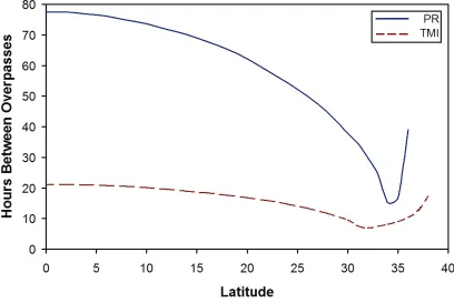
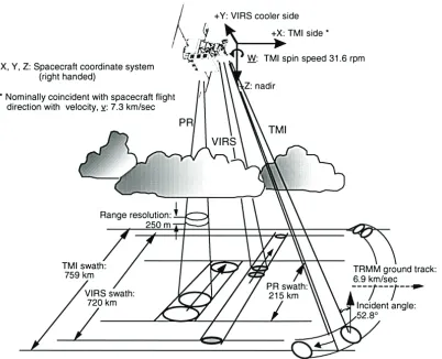
Figure 2.1 Hours between when any part of the instrument swath samples a given point for the PR (solid) and TMI (dashed). The PR has a swath width of 247 km and the TMI has a swath width of 872 km. ...16 Figure 2.2 Schematic view of the scan geometries of the three TRMM primary
rainfall sensors: TMI, PR, and VIRS (from Kummerow et al. 1998)...17 Figure 2.3 TRMM Microwave Imager footprint characteristics (from Kummerow
1998). Features to scale...18 Figure 2.4 Schematic of the data processing flow for TRMM products based on the
VIRS, TMI, and PR instruments...19 Figure 2.5 Simplified schematic of TMI scan geometry. Low resolution channels
appear as shaded circles. High resolution channels appear as open circles in front of the shaded circles. The dots indicate continuation. Features are not to scale with actual IFOVs. (adapted from the TSDIS user’s guide) ..20 Figure 2.6 Calculated brightness temperatures as a function of rainfall rates for five
different freezing levels from 1-5 km. The upper panel is for 19V and the lower panel is for a linear combination of 19V and 22V. The incidence angle is 53 degrees in both panels (from Wilheit et al. 1999). ...21 Figure 3.1 Precipitation characteristics at Kwajalein. Statistics are for 24,285 radar
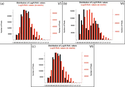
volumes (July- Dec 1999). (Figure courtesy of SE Yuter) ...26 Figure 3.2 PDFs for TRMM V5 and V6 regional oceanic rain rates. Rain rates from
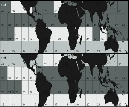
PR are in red and from the TMI swath overlapping PR are in black. PDFs represent accumulated statistics of instantaneous rain rates for 47 days of orbit products from 16 June – 1 August 2001 (pre-boost). (a) V5 Tropical Western Pacific near Kwajalein. (b) V6 Tropical Western Pacific near Kwajalein. (c) V6 Southwest Pacific between Australia and New Zealand.27 Figure 3.3 Map of oceanic regional PDF shape for 47 day accumulated V6 TMI
2001. (b) NH winter from 1 Jan – 16 Feb 2002. Grid numbers are in lower left corner of each grid box...28 Figure 3.4 Shallow precipitation along the northern Morocco coast on 19 September
1999. (a) Surface mask used in 2A-12: land, coast, and ocean. (b) TMI precipitation retrieval with coast/ocean surface border overlaid. (c) PR near surface precipitation...29 Figure 3.5 Views from different sensors of Hurricane Ophelia straddling the North
Carolina coast at ~1400 UTC on 14 September 2005. (a) TMI precipitation retrieval with coast/ocean surface border overlaid. (b) Surface mask used in 2A-12: land, coast, and ocean. (c) PR near surface precipitation. (d) Combined radar reflectivity from coastal NWS WSR-88D radars at Morehead City, NC and Wilmington, NC. (e) TMI precipitation ice at 2000 m about the surface. (f) TRMM 2A-25
precipitation ice at 3500 m above the surface...30 Figure 4.1 Phantom precipitation off the Atlantic Coast of the southeastern US on 18
March 2005. (a) TMI surface precipitation retrieval. (b) PR near surface precipitation. (c) 14 km TMI cloud ice above observed cloud top level. (d) Coastal S-band radar composite. Rings denote maximum range. ...44 Figure 4.2 Skew-T diagram of the Charleston, SC sounding and GOES IR satellite
image for 12Z 18 March 2005. Sounding location indicated on satellite image by green circle. Red line indicates cloud top height. ...45 Figure 4.3 Phantom precipitation off the Atlantic Coast of the southeastern US on 5
March 2002. (a) TMI surface precipitation retrieval. (b) PR near surface precipitation. (c) 8 km TMI cloud ice above observed cloud top level. (d) Coastal S-band radar composite. Rings denote maximum range. ...46 Figure 4.4 Skew-T diagram of the Key West, FL sounding and GOES IR satellite
image for 00Z 6 March 2002. Sounding location indicated on satellite image by green circle. Red line indicates cloud top height. ...47 Figure 4.5 Phantom precipitation off the Taiwan coast on 1 Feb. 2000. (a) TMI
TMI cloud ice above observed cloud top level. (d) Coastal S-band radar composite. Ring denotes maximum range...48 Figure 4.6 Skew-T diagram of the 00Z sounding from northern Taiwan for 1 Feb.
2000...49 Figure 4.7 Phantom precipitation off the Taiwan coast on 1 Feb. 2000. (a) TMI
surface precipitation retrieval. (b) TMI 19V brightness temperature. (c) TMI 37V brightness temperature. (d) TMI 85.5V brightness temperature. The red boundary represents the edges of the phantom precipitation areas and is overlaid over the TMI temperature brightness panels...50 Figure 4.8 The monthly and annual percentage of TMI pixels per 1º x 1º box that
have the radiative signature of phantom precipitation clouds as outlined in section 4.2 for 2002 between 40ºN and 40ºS...53 Figure 4.9 Comparison of plots of the percentage of TMI pixels per 1º x 1º box that
have the radiative signature of phantom precipitation clouds as outlined in section 4.2 with (top) and without (bottom) the TMI rain rate restriction pixels for January 2002 between 40ºN and 40ºS. ...54 Figure 4.10 The monthly and annual means of liquid-phase cloud optical thickness for
2002 between 40ºN and 40ºS as observed by MODIS on the Terra
satellite. ...59 Figure 4.11 The monthly means of latent heat flux for 2002 between 40ºN and 40ºS
from reanalysis data. ...62 Figure 4.12 Edge detection of cloud edges from visible and IR TRMM imagery
overlaid a plot of TMI surface rainfall for a phantom precipitation case off the coast of Taiwan images (red and green lines)...63 Figure 4.13 Six skew-T diagrams of soundings for known phantom precipitation
events. Each sounding illustrates a liquid-phase cloud at least 3 km deep.64 Figure 4.14 Critical number concentrations for the autoconversion of cloud droplet to
and green lines respectively. The thickness ranges of phantom precipitation and typical clouds are denoted by the orange and purple boxes respectively. For autoconversion from cloud droplets to rain droplet to occur, the number concentration must be less than the critical number concentration...65 Figure 4.15 LWC versus cloud thickness for different LWPs. The observed thickness
range of phantom precipitation clouds is denoted by the pink box. The range of TMI observed LWP is denoted by the green area. The area of intersection between the pink and green areas suggest a typical LWC if 0.1 to 0.4 g/m3. ...66 Figure 5.1 (a) Regional map of SeaWiFS-derived chlorophyll a concentration derived
from monthly data for January 2000 to December. Dashed box indicates area of Figure 5.2. Red box indicates MN06’s bloom area and the white box indicates low-bloom area from which time series in (b) and (c) are respectively derived. White areas denote land or missing data. (b) Time series of monthly chlorophyll a concentration and Re as observed by
SeaWiFS and MODIS, respectively, for an area averaged from 49° S to
54° S and 41° W to 35° W (red box). (c) Time series of monthly
chlorophyll a concentration and Re as observed by SeaWiFS and MODIS
respectively for an area averaged from 52° S to 57° S and 55° W to 49° W (white box)...73 Figure 5.2 The 4 week average chlorophyll a concentration derived from 8-day
concentration and Re as observed by SeaWiFS and MODIS, respectively,
for an area averaged from 57° N to 52° N and 150° E to 156° E. ...75 Figure 5.4 Area-averaged time series of MODIS cloud fraction and Re from March
Chapter I – Introduction
Numerical weather prediction and climate analysis on a global scale are
impossible to do properly without meteorological observations over the oceans. Despite the multitude of surface based direct and remote sensing tools available, a satellite remains as the only platform capable of facilitating the reliable and consistent
measurement of meteorological variables over the vast oceans that cover the majority of the planet’s surface.
Since the 1960’s, satellites have been providing measurements and improving almost every aspect of atmospheric study. A classic example of a program that would not exist without satellite derived precipitation estimates is the Global Precipitation
Climatology Project (GPCP). Before satellite estimations of precipitation began, global estimates of the distribution of rainfall – essential for characterizing the global water and energy budgets – were dependant upon the interpolation of data from rain gauges from coastal areas and islands to fill in the data gaps over the oceans where the placement of land based instruments is impossible. These early estimates were coarse and error and uncertainty were high. Even after early forms of satellite based precipitation estimation based on visible and infrared techniques were developed, the standard deviation of monthly rain amounts in tropical locations was comparable to the mean value (Thiele, 1987).
Since proper estimations of tropical rainfall were vital to an accurate
characterization of global water and energy budgets, a specialized satellite program was proposed in the late 1980s to measure precipitation in the tropics using state-of-the-art instruments and techniques to improve the accuracy of the estimates of the distribution and variability of tropical rainfall (Simpson et al., 1988). The Tropical Rainfall
Measuring Mission (TRMM) satellite had the first precipitation radar deployed in space along with the highest resolution passive microwave radiometer ever built at the time of launch (Kummerow et al., 1998).
global circulation in order to predict rainfall and variability at various periods of time; and to test, evaluate, and improve satellite rainfall measurement techniques
(http://tsdis.gsfc.nasa.gov/tsdis/tsdis_redesign/TRMMBackground.html).
1.1 Motivation
It is around the final TRMM goal – the testing and evaluation of satellite techniques – that this study revolves. Validation of satellite data involves making sure that observations are accurate, consistent, and the results based on those observations or combinations of observations are correct.
Satellite algorithms are occasionally updated in an effort to improve performance metrics. As part of evaluating a new algorithm, an effort must be made to ensure that the algorithm does not improve globally at the expense of regional performance or vice versa. Additionally, satellite observations need to be compared to other observations to ensure that they are consistent with physical reality. It is not enough that a satellite sensor returns the correct rain rates and amounts. It must do so for the correct reasons and accurately reflect the physical processes that drive rainfall. Furthermore, it is also importance to look at the nature of the data being collected and determine what circumstances and locations the data is best suited for. As pressure builds to apply
satellite datasets to a variety of applications across different and wide-ranging spatial and temporal scales, it is important to know if the data being collected is suitable for use in a particular application.
An invaluable tool in validating satellite data is inter-sensor comparison. The TRMM satellite has two instruments that make independent rainfall estimations. This is advantageous insofar as the instruments have observational domains that are collocated both spatially and temporally. Differences between the observations of the TRMM satellite’s instruments point to potential errors in the observations of one or both instruments.
errors and inconsistencies in the current TRMM data can be used to help improve GPM data before the program even begins data collection.
1.2 Objectives
The goal of this study is to ensure that satellite estimations of precipitation and cloud characteristics are accurate and consistent across different locations. This study also evaluates several theories present in scientific literature based on satellite
observations of precipitation and cloud characteristics to determine their reproducibility. Specifically, this study aims to do the following:
1. Evaluate the accuracy and consistency of TRMM precipitation estimates over coastal areas
2. Investigate spurious marine precipitation in TRMM TMI dataset and ascertain the role of aerosols, if any, in its presence
3. Test the theory that aerosol produced by phytoplankton can play a dominate role in modifying the properties of marine shallow clouds for a variety of times and locations
Chapter II gives detailed descriptions of the TRMM goals, satellite, instruments, and products with a focus on how the TRMM hardware and software are designed to meet mission goals. Furthermore, Chapter II gives a brief overview of the principles of passive microwave remote sensing of precipitation
Chapter III gives describes changes in the performance of the rainfall retrieval algorithms over time and the continuing need for validation and algorithm refinement. Included in Chapter III is an overview of discontinuities in surface rainfall produced by the TMI over coastal regions and inconsistencies in the TMI derived hydrometeor profile.
Chapter IV describes areas of “phantom precipitation” – areas of rainfall detected by the TMI but not the PR. Chapter IV also evaluates the hypothesis put forth by Berg et al. (2006, hereafter B06) that differences in rainfall detection between the PR and TMI over the East China Sea are due to aerosol loading. IR satellite observations, balloon soundings, and surface based S-band precipitation radar are used to evaluate this
Chapter V examines a proposed correlation, put forth by Meskhidze and Nenes (2006, hereafter MN06), between low liquid-phase cloud effective radius and high chlorophyll a concentration as estimated by the MODIS and SeaWiFS satellite
instruments respectively. The MN06 results are reproduced for their location and time period and then the MN06 hypothesis is tested on a larger dataset to determine if it is reproducible. The evaluation of the MN06 results continues the investigation of the characteristics of low top liquid-phase clouds over the oceans.
Chapter II – The TRMM Satellite
Launched in 1997, the TRMM satellite is a joint effort between NASA and the Japanese Space Agency to improve the estimation and characterization of tropical rainfall. Tropical rainfall plays an important role in the global energy and hydrological budgets. Approximately three-fourths of the energy that drives global circulation comes from latent heat released into the atmosphere by precipitation and two-thirds of that precipitation falls in the tropics of which 75 percent is ocean.
Before satellite observations of weather began, oceanic tropical precipitation was estimated by extrapolation from coastal and island rain gauges, many of which were hundreds or thousands of miles from their closest neighbor. Early satellites made precipitation estimates based on cloud top characteristics derived from visible and infrared imagery (Griffith et al. 1978). Arkin, in a series of studies stemming from the GARP Atlantic Tropical Experiment (GATE), found a correlation between cold IR cloud temperatures and area-average surface rainfall (Arkin, 1979; Richards and Arkin, 1981; Arkin and Meisner, 1987). The correlation was best for the largest temporal scale (1 day) and the largest spatial scale (2.5º x 2.5º) used in the study. Satellite IR rainfall estimates use empirical relationships to determine rain rates based solely on cloud top
temperatures. For instantaneous data with much smaller spatial and temporal scales than used by Arkin, the correlations between IR cold cloudiness and surface rainfall are poor (Yuter and Houze 1998).
Satellite IR estimates of rainfall have some severe limitations. Since IR
observation only collects temperature brightnesses from the tops of clouds, IR techniques can fail in instances where rainfall has dissipated underneath. IR based precipitation estimation schemes, such as the GOES Precipitation Index (Arkin and Meisner 1987), integrated the statistical relationship between IR temperature brightness and surface rainfall over time and space to minimize the effect of these errors. Since that statistical relationship breaks down for instantaneous observations, this study relied on an alternate form of precipitation estimation to evaluate instantaneous data.
et al. 1988). The TRMM satellite carries a precipitation radar (PR) – the first in space – and a passive microwave radiometer – TRMM Microwave Imager (TMI) (Kummerow et al. 1998). Both instruments are capable of obtaining information about the vertical
structure of a precipitating cloud, not just the cloud top like previous satellite instruments. The TRMM program has provided much needed quantitative information about tropical rainfall and, as a result, has improved one of the greatest areas of uncertainty affecting numerical weather prediction, climate research, and hydrological research.
The TRMM satellite is in a low earth orbit at an inclination angle of 35º. This inclination allows the TRMM satellite to make observations as high as 40º latitude with the TMI and 37 º latitude with the PR owing to the inclination of the orbit and the
scanning swath size of the TRMM satellite’s instruments. The TRMM satellite, due to the nature of the low inclination orbit, will sample the full diurnal range of a given area roughly once every 47 days. The TRMM satellite was placed at an orbital altitude of 350 km and had a projected mission life of 3 years.
Due to the success of the TRMM program and the desire for continuing research, the satellite was raised to an orbital altitude of 402 km in August of 2001 in an effort to increase the lifetime of the TRMM satellite and mission. TRMM is currently funded through 2009 with the option for continued funding pending NASA approval and the continued physical wellbeing of the satellite’s instruments.
2.1 TRMM Instrumentation
The TRMM satellite carries 5 different instruments, two of which, the PR and the TMI, are designed specifically to estimate tropical rainfall. The Visible and Infrared Radiometer (VIRS) acts as an auxiliary instrument that can provide additional data if further refinement of rainfall products is needed or if additional data is required beyond that which are provided by the PR and TMI. Figure 2.2 shows a schematic of the scan geometry for the VIRS, the PR, and the TMI. More detailed information about the TMI and PR, the primary TRMM instruments used in this study, is provided below.
2.1.1 TRMM Microwave Imager (TMI)
The TMI is a nine-channel passive microwave radiometer whose design derives from the successful Special Sensor Microwave/Imager (SSM/I) from the Defense Meteorological Satellite Program. The TMI has a rotating offset parabola antenna which scans in a conical pattern with a nadir of 49 degrees resulting in an incident angle of 52.8 degrees with the earth’s surface. The TMI scans a swath below the satellite of 872 km (post-boost).
lower frequency channels. Figure 2.3 shows the characteristics of the TMI’s EFOV and how it is derived from the IFOVs. Table 2.1 outlines the performance characteristics for each channel.
2.1.2 Precipitation Radar (PR)
The PR is a 13.8 GHz frequency precipitation radar and was the first precipitation radar in space. The PR uses a 128-element phased array transmitter/receiver to scan a 247 km (post-boost) swath below the satellite with a nadir pixel horizontal resolution of 4.9 km and a vertical resolution of 250 m. The PR has a minimum sensitivity of ~18 dBZ. The wavelength and transmitting power of the PR make it prone to attenuation in moderate to heavy rainfall and hail. Attenuation increases the uncertainty of rainfall measurements. However, for rainfall rates < 10 mm/hr, the uncertainty posed by attenuation is minimal.
2.1.3 Visible and Infrared Radiometer (VIRS)
The VIRS is a five-channel imaging spectroradiometer with bands in the
wavelength range from 623 nm to 12.028 micrometers spanning the visible and infrared portions of the electromagnetic spectrum. The VIRS scans a 827 km swath below the satellite with a nadir horizontal resolution of 4.85 km. The VIRS provides cloud-top temperatures to complement the passive and active microwave measurements from the TRMM satellite. Additionally, the IR measurements available from the TRMM platform allow the microwave measurements to be compared and contrasted with established, geostationary satellite IR techniques for rainfall retrieval.
2.2 TRMM Products
TRMM satellite data is distributed in the hierarchical data format (HDF). There are 3 levels of data products which vary in complexity ranging from level 1 data which includes raw sensor output, to level 3 data which can include gridded data processed with information taken from multiple level 1 and level 2 products and integrated over
satellite instruments. Level 2 data consists of variables and products computed from level 1 data that remains at the same spatial and temporal scale. Level 3 data combines
multiple orbits of level 1 and level 2 data to produce gridded products across a global domain with a longer temporal domain than level 1 or level 2 data. Figure 2.4 shows a schematic of the data processing flow the TRMM products based on the VIRS, TMI, and PR instruments. The level 3 data is built upon the level 2 data which is built on the level 1 data. Detailed information about the TRMM products used in this study follows.
2.2.1 1B01 – VIRS Calibration
The TRMM 1B01 product contains the calibrated temperature brightness values for each of the VIRS's five channels. 1B01 records 261 EFOVs per VIRS scan line. In addition to the calibrated VIRS brightness temperatures, the 1B01 data product contains calibration information and coordinates for geospatial registration.
2.2.2 1B11 – TMI Calibration
The TRMM 1B11 product contains the calibrated temperature brightness values for each of the TMI's nine channels. The values for each channel are split across two datasets. The lower resolution channels, consisting of the frequencies 10.65 GHz, 19.35 GHz, 21.3 GHz, and 37 GHz, occupy their own dataset owing to their larger EFOV compared to the 85.5 GHZ channels. The low resolution dataset has half the number of points per scan line (104) as the higher resolution dataset (208). The two TMI channels at 85.5 GHz occupy the high resolution dataset. Figure 2.5 shows a simplified version of the scan geometry for two scans illustrating how the high resolution and low resolution channels overlay. In addition to the calibrated TMI brightness temperatures, the 1B11 data product contains calibration information and coordinates for geospatial registration.
2.2.3 2A12 – TMI Rainfall
water, precipitation ice, cloud water, cloud ice, and information about the background surface type. 2A12 also contains coordinates for geospatial registration.
2.2.4 2A23 – PR Qualitative
The TRMM 2A23 product contains assorted qualitative information about the type of rain being observed as well as some statistics about the bright band information. 2A23 specifies the depth of rainfall, convective or stratiform characteristics, as well as water phase information. 2A23 also contains information about the location and intensity of the bright band. Additionally, 2A23 contains coordinates for geospatial registration.
2.2.5 2A25 – PR Profile
The TRMM 2A25 product contains the derived rainfall and reflectivity
information as calculated by the PR rainfall processing algorithm from the 1B21 product. 2A25 contains PR derived near-surface rainfall, near-surface reflectivity, the profiles of rainfall, the three-dimensional distribution of reflectivity, and myriad data on PR attenuation and error corrections. 2A25 also contains coordinates for geospatial registration.
2.3 Passive Microwave Radiometry
2.3.1 Radiation and Emissivity
All substances emit radiation in amounts governed by their thermal energy and material properties. The Stefan-Boltzmann law states that, assuming all other things are equal, the warmer a substance, the more energy it will radiate. A blackbody is a
theoretical substance that is a perfect emitter. A blackbody will emit the maximum amount of energy for its temperature as described by the Stefan-Boltzmann law.
wavelength will emit 50% of the energy as a blackbody at the same temperature and at the same wavelength.
2.3.2 Rainfall Emission
The TMI infers rainfall rates by measuring upwelling microwave radiation at different frequencies. The amount of radiation measured is expressed in terms of brightness temperature. Plank’s Law describes how much radiation is emitted by a blackbody for a given temperature and wavelength. Using Plank’s Law, the amount of radiation measured at the satellite at a given wavelength is used to calculate the temperature of the observed location assuming that it behaves as a blackbody. This temperature is called the brightness temperature. Depending on the emissive properties of the location being observed, the brightness temperature may be close to the actual
temperature for a high emissivity location or the brightness temperature may not be close to the actual temperature for a low emissivity location.
The observed brightness temperature from a satellite is dependent on the emission from the earth’s surface modified by the intervening atmosphere. The oceans emit only about 50% of the microwave energy as an equivalent blackbody surface. Thus, by using the concept of brightness temperature, the oceans can be considered to appear uniformly cold in passive microwave observations. Rainfall emits microwave energy based on its true temperature - the atmospheric wet-bulb temperature - and appears much warmer than an ocean background owing to radiative differences between suspended droplets versus a plane surface. The lower frequency band of the microwave spectrum (10-37 GHz) is the most sensitive to rainfall emission. For a given situation, the deeper the rain layer and the more intense the rainfall (the greater the liquid water path) the warmer the brightness temperature observed over a cold ocean background will be. Complicating factors to this idealized relationship are partially melted ice particles, atmospheric variability, and other variables as described by Wilheit (1991).
Figure 2.6 shows the relationship between brightness temperature and surface rain rate for different freezing level (rain layer depth) used by an early emission based
saturation occurs at higher rain rates for lower microwave frequencies. A multi-spectral approach to surface rainfall estimation helps to reduce the uncertainty in translating temperature brightness to a specific surface rain rate.
Microwave emission based estimates of rainfall encounter problems when applied over land. Land surfaces, like rainfall, have a high emissivity and emit microwave energy based on their thermodynamic temperature and do not have a low emissivity like an ocean surface which has a brightness temperature much lower than its thermodynamic temperature. For example, a 300 K land surface will have a brightness temperature close to 290 K while a 300K ocean surface would have a brightness temperature near 165 K. As a result, microwave emission from rainfall is almost impossible to distinguish from microwave emission from a land surface. While a warm spots stands out over a cold background (rain over ocean), a warm spot does not stand out over an equally warm background (rain over land). The emission signal from the rainfall is not detectable over the background noise of the land emission.
2.3.3 Ice Scattering
Cloud ice particles have a different effect on microwave observations than rainfall. While rainfall emits microwave energy, cloud ice particles scatter upwelling microwave radiation. The more scattering of upwelling radiation that occurs, the closer the observed brightness temperature approaches the background microwave temperature brightness of outer space. Similar to how low frequency microwave observations are most sensitive to rainfall emission, high frequency microwave observations (37-85.5 GHz) are most sensitive to sized ice particle scattering. While precipitation-sized ice does not have a direct physical link to surface rainfall, it can provide some information about the vertical hydrometeor structure of a cloud. Additionally, since the signal of ice particle scattering is the same over land or ocean, scattering based
estimations of rainfall are less prone to surface type ambiguities that emission based estimations experience over land.
temperatures in high frequency channels (37 GHz and 85.5 GHz). Note that the 37 GHz channel is sensitive to the signal from emission and scattering where 10.65 GHz is sensitive to purely emission and 85.5 GHz is sensitive to purely scattering. By making passive microwave observations at different frequencies, information can be gathered about the amount of rainfall, liquid cloud droplets, and frozen cloud droplets in a given cloud.
2.4 Passive Microwave Retrieval Algorithms
Microwave rainfall retrieval algorithms can use measured brightness temperatures to determine a surface rainfall rate via two different methods: empirical and physical.
Empirical methods use multivariate regression relationships between observed brightness temperatures and ground-based rainfall measurements to arrive at a surface rainfall. The largest drawbacks of empirical algorithms lies in the fact that they are not based on and do not provide any physical insight into the atmosphere and the variables and physical characteristics that determine rainfall amounts. Furthermore, there is no guarantee that the empirical relationships between brightness temperatures and rain rates will be valid outside of the observational area where the relationships were established.
Physical methods of rainfall retrieval make use of radiative transfer and cloud microphysics models. A radiative transfer model uses thermodynamic and hydrometeor profiles of the atmosphere to estimate top of atmosphere brightness temperatures. The hydrometeor profiles input to the radiative transfer model are produced by cloud models, and each profile has an associated surface rainfall. The accuracy of physically based algorithms is critically dependant on the accuracy of the assumptions of the
microphysical parameters and the realism of the cloud model simulation for the case being observed.
2.4.1 The Goddard Profiling Algorithm
temperature brightnesses are observed by the TMI, a Baysian retrieval function matches the observed brightness temperatures to the brightness temperatures of an event in the GPROF database that best fits the observed values. The theory is that the modeled event retrieved from the database is representative of the event being observed by the TMI and the properties of the database event are used to provide details such as rain rate and microphysical properties.
TMI rainfall estimation based on the GPROF database has some important limiting factors. Vertically-integrated brightness temperatures are used to select a relevant hydrometeor profile from the GPROF database. However, Wilheit (1991) said that there is not a one-to-one mapping between sets of brightness temperatures and hydrometeor profiles, i.e. that different hydrometeor profiles can yield the same set of brightness temperatures. It is possible that the event returned by GPROF could be drastically different the event being observed. Information that could help distinguish precipitation structures such as the size of the contiguous rain area in which the column is embedded is not included in the current algorithm.
A related issue concerns observation of events not contained in the GPROF database. The GPROF database is large, - with simulations based on the TOGA COARE, GATE, and COHMEX field studies - but still finite and cannot possibly contain model simulations of every conceivable meteorological situation. As a result, the GPROF database for the TMI contains the most commonly observed kinds of events most likely to be observed during the TRMM mission; primarily deep tropical convection. If the TMI observes a situation not represented in the GPROF database, the algorithm is forced to guess from among the cases it does represent. This situation will result in the TMI algorithm returning potentially inaccurate rain rates and non-physical hydrometeor profiles.
Table 2.1 TMI per channel characteristics. DT denotes down-track values. CT denotes cross-track values. (Adapted from Kummerow et al. 1998)
TMI Channel Characteristics
Channel Number 1 2 3 4 5 6 7 8 9
Frequency (GHz) 10.65 10.65 19.35 19.35 21.3 37.0 37.0 85.5 85.5
Polarization V H V H V V H V H
Beamwidth (deg) 4.23 4.31 2.18 2.16 1.95 1.15 1.15 0.52 0.53 IFOV-DT (km) 67.8 69.0 35.0 34.6 31.2 18.4 18.4 7.7 7.9 IFOV-CT (km) 41.0 41.8 21.1 20.9 19.0 11.1 11.1 4.7 4.8 EFOV-DT (km) 10.5 10.5 10.5 10.5 10.5 10.5 10.5 5.3 5.3 EFOV-CT (km) 72.6 72.6 34.9 34.9 25.9 18.4 18.4 8.3 8.3
Chapter III – TMI Coastal Rainfall Discontinuities
3.1 Error Characteristics for TRMM Products
The TRMM satellite precipitation retrieval algorithms have undergone a series of refinements since launch that have been released intermittently and labeled with different version numbers. TRMM Version 5 (V5) was released in November 1999 and Version 6 (V6), the most recent version, was released in April 2004. While the changes
incorporated into each new version are intended to improve the accuracy and precision of TRMM products, they do not always do so across all metrics. The impact of precipitation retrieval errors varies with the product application. Yuter et al. (2005) examines the changes between V5 and V6.
Error characteristics associated with satellite-derived precipitation products are important for the use of TRMM products in atmospheric and hydrological model data assimilation, forecasting, and climate diagnostics applications. Additionally, this information aids in the diagnosis and refinement of physical assumptions within algorithms by identifying geographic regions and seasons where existing algorithm physics may be incorrect or incomplete. Examination of relative errors between
independent estimates derived from satellite passive microwave and precipitation radar is particularly important over regions with limited surface-based measurements of rain rate such as the global oceans and tropical continents. Ground-based observations at selected sites can help guide the physical interpretation of the error characteristics. The analysis of TRMM satellite datasets yields error information on the current TRMM products and is also an opportunity to prototype error characterization methodologies for the TRMM follow-on program, the Global Precipitation Measurement mission (GPM).
3.2 Data Sets
The TRMM satellite data sets were processed to yield several types of relative error statistics in this study. We also examined the plausibility of the TRMM products compared to existing empirical knowledge. TMI and PR instantaneous rain rates are compared over ocean and land using orbit data from V6 TRMM products 2A-12,
representing the TMI rainfall retrieval, and 2A-25, representing the PR rainfall retrieval. Within the TMI instantaneous algorithm 2A-12, 85 GHz and 19 GHz are the heaviest weighted channels over ocean and land, respectively (Kummerow et al. 1996). We use the “near surface” values for rain rates, which are available in both V5 and V6 products.
Level 2 WSR-88D radar data from the National Climatic Data Center and the Central Weather Bureau of Taiwan was processed for comparison to TRMM products. The radar data was processed through a quality control program to unfold radial velocities and remove non-meteorological echoes. The data was then interpolated to a 240 km by 240 km Cartesian grid with 3 km horizontal resolution and 3 km vertical resolution.
3.3 TMI Regional Probability Density Functions (PDFs) of Rain Rate
Yuter et al. (2005) examined the PDFs of surface rainfall which yields both quantitative information about potential error and information about physical plausibility. Figure 3.1 shows the PDF of the radar reflectivity of tropical precipitation as observed in the KWAJEX field study in 1999. Log10 of rainfall rates have a similar distribution
structure as radar reflectivity in dBZ since dBZ=b log10 (R)+a where a and b are
constants and R is rain rate. Observed rainfall rates in this region are unimodal with an approximately Gaussian distribution.
The corresponding PR V5 and PR V6 PDFs are unimodal. Many regions with heavy tropical precipitation during the summer season, such as the tropical western Pacific near Kwajalein, show problematic bimodal PDFs in V6 TMI (Figure 3.2b) that were not present in V5 (Figure 3.2a). Some PDFs at higher latitudes also exhibit bimodal characteristics, such as the western Atlantic off the US coast (Figure 3.3). Other PDFs have the expected unimodal characteristics, such as the southwest Pacific between the east coast of Australia and New Zealand during the local winter (Figure 3.2c). Figure 3.3 shows the geographic distribution of the various PDF modes in June and January. The bimodal PDFs occur more often in local summer months and in regions of intense precipitation such as the Intertropical Convergence Zone (Yuter et al., 2005). To better understand the causes of the differences between global oceanic and land PDFs storms that span the coast line are examined in the next section.
3.4 TMI Spatial Discontinuities
Over the ocean, both scattering and emission channels are used to derive the TMI rain rate. Over the land and coast, the satellite-observed emission from precipitation is contaminated by emissions from the surface. Because the emission signal from heavy rainfall over land cannot be readily distinguished from radiation emitted from the land surface, the rainfall retrieval algorithms for the TMI must rely heavily on the scattering signal from ice. As a result, the TMI emission channels are not weighted heavily over land and are not used at all over coast (Kummerow et al. 1996). The different sets of information available to the precipitation retrieval algorithms for land and coast versus ocean can lead to discontinuities in the retrieved precipitation field.
However, for cases over land with a large amount of ice scattering, the TMI still has problems. Figure 3.5 compares the precipitation retrieval from the TRMM PR and the TMI for Hurricane Ophelia over the North Carolina coast. The TMI retrieved rain rate field has abrupt discontinuities along the boundaries between ocean and coast (Figure 3.5a). These discontinuities are not observed in either the TRMM PR derived rain rates or the near-surface reflectivity obtained by National Weather Service (NWS) WSR-88D radar. In the Ophelia case, the limited information from the 85.5 GHz channels leads to an underestimation of rainfall rates over land surfaces and spatial errors when locating areas of intense rainfall. The size and shape of the eye of the hurricane in the TMI rain field is also inconsistent with the PR and WSR-88D observations. Disagreement between the TMI and PR indicates observational and processing errors in one or both instruments. These inconsistencies lead to errors in the data and analyses that are derived from the TRMM observations.
Within the TMI 2A-12 algorithm, vertical profiles of hydrometeors are associated with the observed TMI brightness temperatures and estimated surface rain rates. Profiles of cloud liquid water, precipitation liquid water, cloud ice, and precipitation ice are included as part of the 2A-12 product. The hydrometeor profiles provide a valuable diagnostic of an intermediate step within the TMI algorithm.
Figure 3.1. Precipitation characteristics at Kwajalein. Statistics are for 24,285 radar volumes (July- Dec 1999). (Figure courtesy of SE Yuter)
Figure 3.2. PDFs for TRMM V5 and V6 regional oceanic rain rates. Rain rates from PR are in red and from the TMI swath overlapping PR are in black. PDFs represent
accumulated statistics of instantaneous rain rates for 47 days of orbit products from 16 June – 1 August 2001 (pre-boost). (a) V5 Tropical Western Pacific near Kwajalein. (b) V6 Tropical Western Pacific near Kwajalein. (c) V6 Southwest Pacific between Australia and New Zealand.
Figure 3.3. Map of oceanic regional PDF shape for 47 day accumulated V6 TMI
instantaneous rain rates. Color coding indicates unimodal (medium grey), bimodal (dark grey), and strongly skewed (light grey) distributions in log10(R). (a) Northern Hemisphere
(NH) summer from 16 June – 1 August 2001. (b) NH winter from 1 Jan – 16 Feb 2002. Grid numbers are in lower left corner of each grid box.
Figure 3.5. Views from different sensors of Hurricane Ophelia straddling the North Carolina coast at ~1400 UTC on 14 September 2005. (a) TMI precipitation retrieval with coast/ocean surface border overlaid. (b) Surface mask used in 2A-12: land, coast, and ocean. (c) PR near surface precipitation. (d) Combined radar reflectivity from coastal NWS WSR-88D radars at Morehead City, NC and Wilmington, NC. (e) TMI
Chapter IV - Phantom Precipitation
The investigation of surface discontinuities over coastal areas led to the incidental discovery of a different phenomenon in TMI rainfall estimations. There were regions of light but widespread precipitation in the TMI products that were not in the corresponding PR observations. Surface-based instruments also did not indicate rainfall in the area where TMI indicated rainfall. These areas of seemingly mistaken precipitation were dubbed “phantom precipitation”.
Phantom precipitation is defined as a widespread area of surface precipitation over the ocean, indicated by the TMI 2A12 product, which does not exist in reality. We have identified many cases of phantom precipitation. TMI reported phantom precipitation rain rates can exceed 2 mm/hr and have a mode that varies from case to case ranging from 0.6 – 1.2 mm/hr. Figure 4.1 shows a large area of precipitation off the US Atlantic Coast from TMI that was not present in the corresponding PR observations. There is a unimodal distribution of rain rates in the phantom precipitation areas. TMI returned rain rates for phantom precipitation areas lie within a range easily detectable by coastal S-band radar. Reflectivity data from the five National Weather Service WSR-88D radars nearest the coast to the phantom precipitation area were composited together. The coastal S-band radars were unable to detect any precipitation returns corresponding to phantom precipitation areas within the observational range of the WSR-88D radars (~240 km) (Figure 4.1d).
Figure 4.3 shows a large area of precipitation indicated by the TMI off the southern Florida coast that was not present in the corresponding PR observations. The TMI rain rates in this case were unimodal with a mean of approximately 0.6 mm/hr and well above the minimum detectable rain rate of a NWS WSR-88D radar. Reflectivity data from the two National Weather Service WSR-88D radars nearest the coast to the
phantom precipitation area were composited together. The coastal S-band radars were unable to detect any precipitation returns corresponding to phantom precipitation areas within WSR-88D observational limits (Figure 4.3d).
Based on analysis of GOES IR imagery (Figure 4.4), the phantom precipitation off the southern Florida coast also occurred under liquid-phase stratus clouds. Analysis of upper-air soundings (Figure 4.4) from locations close to the phantom precipitation area reveals a cloud top height of ~4 km that lies just below the freezing level. An
investigation of the TMI returned hydrometeor profiles showed inconsistencies with the observed conditions in the same fashion to the case off the US Atlantic Coast. The TMI indicated a deep layer of cloud ice starting above the observed cloud top and continuing to 18 km in height near the top of the troposphere (Figure 4.3c). As with the US Atlantic Coast case, the TMI algorithm returned a hydrometeor profile that is not physically consistent with the observed conditions.
4.1 Berg et al., 2006
their theory based on observations from Ishizaka at al. (2003). They suggested that for a relatively high liquid water path cloud (1 kg/m2) with a plausible cloud droplet number concentration based on observations of polluted clouds (400 cm-3), the reflectivity could be reduced to approximately 18 dBZ – just below the PR minimum threshold of
detection.
The case examined by B06 is shown in figure 4.5. There is a large area of precipitation indicated by the TMI that is not present in the corresponding PR
observation. An examination of the distribution of rain rates returned by the TMI (not shown) yielded a unimodal distribution with a mode of approximately 1 mm/hr. This distribution of rain rates lies within the range detectable by coastal WSR-88D S-band radar on Taiwan. Examination of the coastal S-band radar data for the case in B06 did not reveal a widespread area of precipitation corresponding to the TMI rainfall area. The reflectivity range corresponding to the TMI rain rates as theorized by B06 (~18 dBZ) would be observable by the coastal S-band radar if the echoes were present (Figure 4.5). The operational minimum detection threshold for the Taiwan radar is 5 dBZ in VCP 21 precipitation mode. The theoretical minimum threshold is -15 dBZ (Miller et al. 1998). The Taiwan coastal S-band WSR-88D radar did not detect any echoes > 10 dBZ in the East China Sea corresponding to features identified as raining in TMI but not PR. The radar observations do not rule out that aerosols may be a contributing factor, but they are not a major contributor to phantom precipitation clouds in the B06 case.
Like other phantom precipitation cases, the B06 case off Taiwan had serious problems with the TMI retrieve hydrometeor profile. Sounding data indicates a cloud top of 3.9 km (Figure 4.6). However, just as in other cases, the TMI indicates a layer of ice phase cloud droplets from the observed cloud top all the way to the top of the troposphere (Figure 4.5c). The incorrect hydrometeor profile is an indication that the TMI algorithm is providing an incorrect physical interpretation of the observed clouds and may be making incorrect assumptions about their characteristics and structure.
4.2 Phantom Precipitation Global Mapping
find a unique identifying signature for phantom precipitation, the TMI temperature brightness from the 1B11 product were examined for each channel of each cases off the US and Southeast Asia coast. A joint brightness temperature distribution among 3 TMI channels, 19V, the 37V, and the 85.5V can be used to distinguish phantom precipitation from the background and other cloud and precipitation features. Figure 4.7 illustrates a phantom precipitation signature in the 19V, 37V, and the 85.5V channels for an example case off the coast of Taiwan. In these channels the area of phantom precipitation is distinguishable from the background pattern. In the other TMI channels, the phantom precipitation area was not readily distinguishable from the background pattern. Edge detection techniques were used to outline the boundaries of the phantom precipitation. The range of brightness values inside the denoted phantom precipitation regions was used to create a filter to separate phantom precipitation areas from non-phantom precipitation areas. For those three channels, the range of brightness temperatures for known areas of phantom precipitation was tabulated. For the 19V channel, the temperature brightness of phantom precipitation was between 195 K and 225 K. For the 37V channel, the
temperature brightness of phantom precipitation was between 230 K and 254 K. And for the 85.5V channel, the temperature brightness of phantom precipitation was between 267 K and 280 K. The set of brightness temperatures for a given TMI pixel must meet the 3 conditions above to be considered as phantom precipitation.
filtered out non-oceanic pixels (i.e. land and coast), pixels not defined as raining by the TMI algorithm, and pixels with rain rate significantly higher that observed in confirmed phantom precipitation cases (3 mm/hr). These last two distinctions were made since phantom precipitation is, by definition, flagged as raining by the TMI, but not classified by raining other instruments. Table 4.1 summarizes the criteria used for the phantom precipitation filtering scheme.
Individual orbits were processed for one month periods. Pixels in each orbit identified as phantom precipitation were sorted into 1 degree by 1 degree boxes between 40 degrees north and 40 degrees south. For a given 1 degree by 1 degree box, each phantom precipitation pixel was counted and, at the end of the monthly computational period, the total number of observed phantom precipitation pixels was divided by the total number of TMI pixels for that box yielding a map of the normalized percentage of TMI observations having a radiative signature similar to phantom precipitation. This data was plotted into maps for each month for 2002. The data for each month was then
combined to create a map of the percentage of TMI observations classifiable as phantom precipitation for all of 2002 (Figure 4.8).
4.3 Global Distribution of Phantom Precipitation
The identification of phantom precipitation in the TMI surface rainfall product quickly leads to questions about the frequency and geographic distribution of phantom precipitation. The global maps of phantom precipitation, calculated and compiled using the methods described above, provided information about the spatial distribution and the temporal frequency of phantom precipitation signatures in the TMI observations for 2002.
Figure 4.8 shows the percentage of TMI observations with phantom precipitation radiative signatures on a 1° by 1° grid for each month in 2002. On a monthly basis, upwards of 30% of TMI observations can have a phantom precipitation radiative
signature depending on the location and time of year. For an annual time scale, phantom precipitation signatures have a global average occurrence rate of 1% but can go as high as 10% in particular regions; most notably off the eastern coast of China northwest of
precipitation seems to occur most commonly in the winter hemisphere on the lee side of continents. It is also noticeable more common at latitudes further than 15° from the equator. Phantom precipitation clouds occur in a variety of areas that are noted for different levels of aerosol pollution, ranging from very polluted areas (e.g. East China Sea) to areas with very low aerosol amounts (e.g. Southern Pacific Ocean). The B06 hypothesis relating their clouds to pollution is inconsistent with their clouds being in low aerosol areas.
For the month of January 2002, the phantom precipitation mapping algorithm was used to create a map of the percentage of TMI observations classifiable as phantom precipitation, but without the restriction of TMI rain rates. The algorithm was unchanged from how described above accept that it no longer filtered out pixels with a TMI rain rate of 0 mm/hr or a TMI rain rate greater that 3 mm/hr. Figure 4.9 shows to maps for January 2002 with and without the restrictions on TMI rain rate. The amounts and distributions of phantom precipitation further than 15- 20 degrees from the equator remain unchanged. However, the map without the restrictions in TMI rain rate indicates a significantly larger amount of frequency phantom precipitation in the vicinity if the ITCZ. This result
suggests that the radiative signal for phantom precipitation may not be consistent for all regions or latitude bands. A known latitude and seasonal sensitivity of the TMI algorithm is freezing level height (rain layer depth) which varies from a maximum level near equator to a minimum level at higher latitudes in the winter hemisphere. The set of
brightness temperatures characteristic of phantom precipitation imply a LWP between 0.5 and 1.2 kg/m2. In the tropics where there is a deep rain layer (~4.5 km) this LWP is
interpreted as not raining while in higher latitude winter where there is a shallower rain layer it is interpreted as raining.
4.4 What is Phantom Precipitation?
Furthermore, we looked at the characteristics we have been able to observe about the physical properties of phantom precipitation clouds to determine what clues they can yield about what sets phantom precipitation clouds apart from other low marine clouds.
4.4.1 Phantom Precipitation Relationship to Environmental Parameters
The monthly and annual average averages for 16 environmental parameters for 2002 were compiled for comparison with the corresponding phantom precipitation maps examined section 4.3. If the spatial features for a given variable correspond with the spatial distribution of phantom precipitation, that variable may be an important factor in causing or maintaining phantom precipitation. By examining the correlations of many meteorological parameters a better picture can be formed of what factors do and do not play a role in phantom precipitation.
The distribution of phantom precipitation was compared to nine cloud characteristic products from the MODIS sensor of the Terra satellite: aerosol optical depth (AOD); cloud effective radius for liquid, ice and mixed phases; optical thickness for liquid, ice, and mixed phases, cloud top pressure, and cloud top temperature. Five environmental variables compiled from reanalysis data was compared to the distribution of phantom precipitation: outgoing longwave radiation (OLR), mean sea-level pressure (MSLP), sea surface temperature (SST), sea surface temperature anomaly, latent heat flux, and omega at 500 mb. Several studies (Shaw, 1983; Charlson et al., 1987;
Middlebrook et al., 1998; O’Dowd et al., 2004) have suggested possible mechanisms by which phytoplankton can influence marine cloud properties. As a result, the distribution of phantom precipitation was compared to chlorophyll a as observed by the SeaWiFs sensor aboard the Seastar satellite. The measurement of chlorophyll a over the ocean acts as a proxy for the detection of phytoplankton. Whether or not any of the above
parameters corresponded with the distribution of phantom precipitation is summarized in table 4.2.
cloud when cloud is present. Liquid phase cloud optical thickness has a weak correlation with phantom precipitation. Liquid phase cloud optical thickness sometimes has local maxima in areas where phantom precipitation has a high frequency of occurrence. However, the local maxima between phantom precipitation and liquid phase optical thickness do not always correspond and in some cases local maxima in liquid phase cloud optical thickness occur where there is a local minimum in phantom precipitation
frequency. Since the correlation in not consistent, this suggests that liquid phase cloud optical thickness is an indicator of moisture rich clouds of which phantom precipitation is only a subset.
Figure 4.11 depicts monthly mean surface latent heat flux as derived from reanalysis data for 2002. Surface latent heat flux describes the flux of heat from the Earth's surface to the atmosphere that is associated with evaporation of water at the surface. High surface latent heat flux correlates with high frequency of phantom precipitation, in some months but not others. Strong evaporative moisture flux would increase the moisture content in the air and lead to lower cloud bases compared to regions with similar air temperature and lower evaporative moisture flux. Surface latent heat flux is strongest in areas known for explosive cyclogenesis (characterized by cool air over warm water). This suggests that the vertical moisture flux from the surface associated with cyclogenesis may contribute to a favorable environment for shallow phantom precipitation clouds in between cyclogenesis episodes.
4.4.2 Phantom Precipitation Cloud Top Properties
Passive microwave observations are vertically integrated observations of clouds. Visible and infrared observations examine only the tops of clouds. To determine if cloud top characteristics can provide clues about the occurrence of phantom precipitation clouds, edge detection techniques were used to determine the outline of cloud features in visible and infrared imagery for known phantom precipitation cases.
the edge of the cloud or a textural change in the cloud top. The features identified in the visible and infrared imagery do not correspond with any edge or pattern in the TMI image. This indicates that phantom precipitation is not cloud top feature, but indicative of a feature of the cloud bottom or a property of the entire cloud volume.
4.4.3 What is Phantom Precipitation: A Cloud Thickness Argument
Analysis of a multitude of environmental parameters and cloud top properties yielded useful information about what phantom precipitation clouds are not. Radar observations have indicated that aerosol modification as described by B06 is not
consistent with other observations.. Sounding data from phantom precipitation cases has shown that phantom precipitation clouds are thicker than the norm expected for shallow marine clouds. We have seen a moderate association of phantom precipitation and areas of high surface latent heat (evaporative moisture) flux. Surface latent heat flux would increase near-surface moisture and facilitate lower cloud bases potentially leading to thicker clouds. A possible explanation of phantom precipitation is that it is the result of abnormally thick low clouds.
Sounding data indicated that phantom precipitation clouds have a cloud top just below the sounding derived freezing level. More interesting is that phantom precipitation clouds have a lifting condensation level – a good proxy for the cloud base – very close to the surface. This means that phantom precipitation clouds are unusually thick. Where a normal marine stratus cloud may have a thickness of 1-2 km, a phantom precipitation cloud has a thickness of 3-4.5 km. Figure 4.13 shows an array of soundings from
observed phantom precipitation events near coastal areas off the US and southeast Asia. These soundings confirm a nominal cloud thickness of 3-4.5 km where the clouds in question extend from near the surface to just below the freezing level.
water content (LWC) than for a thinner cloud. This phenomenon would have a
precipitation suppressing effect similar to the theory of B06, but would also be consistent with satellite, radar, and sounding observations unlike the B06 theory (Figure 4.6).
B06 uses a Kessler-type parameterization based on the work of Liu et al. (2004) and Liu and Daum (2004) to examine the critical radius of autoconversion of cloud droplet to raindrops for different droplet number concentrations and liquid water
contents. B06 states that autoconversion should occur any time the number concentration in a cloud is fewer than
3 / 4 2 63 . 24 L
Nc = (1)
where Nc is the number concentration and L is the liquid water content. The maximum
value of Nc for autoconversion is referred to as the critical number.
The area of phantom precipitation analyzed in B06 off the coast of Taiwan had a LWP of ~1 kg/m2 (Berg et al., 2006). Analysis of other phantom precipitation cases shows that this is a typical value for the LWP of phantom precipitation events and was used in the B06 study. Cloud thickness, LWP and LWC can be related by
LWC=LWP/T (2)
where LWC is the liquid water content in g/m3, LWP is the liquid water path in kg/m2, and T is the cloud thickness in km.
A typical liquid-phase marine cloud can have a thickness of 1.5 km (Wang and Rossow, 1995) and phantom precipitation clouds have been observed to have a thickness 3-4.5 km. Assuming a LWP of 1 kg/m2, this leads to LWC values of 0.8 g/m3 and 0.33 g/m3 respectively for a 3 km thick cloud. According to formula (1) the typical 1.5 km thick cloud would have a critical number concentration of 440.7 cm-3 and the 3 km thick phantom precipitation cloud would have a critical number concentration of 137 cm-3.
“clean” or polluted cloud. This simple analysis shows that for a given LWP differences in cloud thickness can readily explain why a cloud may or may not precipitate.
Figure 4.14 shows a plot of the critical droplet number concentration based on the parameterization described above versus the cloud thickness for different LWP values. Precipitation will occur when the cloud droplet number concentration is less than the critical value given by the relevant curve based on the LWP. For a given cloud thickness, the critical cloud droplet number concentration is higher for a cloud with a higher LWP value. For a given cloud droplet number concentration, a thick cloud would require a higher LWP than a thinner cloud to develop rainfall.
Figure 4.15 shows a plot of LWC for different LWP values as a function of cloud thickness. Observed cloud thicknesses for phantom precipitation cases range from ~3-4.5 km. Phantom precipitation clouds have an observed TMI LWP of ~0.5-1.2 kg/m2 (Berg et al., 2006). As a result, phantom precipitation clouds have a LWC of ~0.1-0.4 g/m3.
Table 4.1. Summary of Phantom Precipitation Filter Scheme Criteria. Summary of Phantom Precipitation Filter Scheme Criteria
Filter Parameter Value Range
19V Temp. Brightness 195-225K
37V Temp. Brightness 230-254K
85.5V Temp. Brightness 267-280K
TMI Near-Surface Rain Rate 0 mm/hr < R <3 mm/hr
Table 4.2. Summary of Phantom Precipitation Correspondence to Environmental Parameters.
Summary of Phantom Precipitation Correspondence to Environmental Parameters
Environmental Parameter Correspondence with Phantom Precipitation
OLR None AOD None
Reff - liquid None
Reff - ice None
Reff - mixed None
Optical Thickness - liquid Partial
Optical Thickness - ice None
Optical Thickness - mixed None
Cloud Top Pressure None
Cloud Top Temperature None
MSLP None SST None
SST anomaly None
Latent Heat Flux Partial
Omega – 500mb None
Figure 4.1. Phantom precipitation off the Atlantic Coast of the southeastern US on 18 March 2005. (a) TMI surface precipitation retrieval. (b) PR near surface precipitation. (c) 14 km TMI cloud ice above observed cloud top level. (d) Coastal S-band radar
Figure 4.7. Phantom precipitation off the Taiwan coast on 1 Feb. 2000. (a) TMI surface precipitation retrieval. (b) TMI 19V brightness temperature. (c) TMI 37V brightness temperature. (d) TMI 85.5V brightness temperature. The red boundary represents the edges of the phantom precipitation areas and is overlaid over the TMI temperature brightness panels.