University of Windsor University of Windsor
Scholarship at UWindsor
Scholarship at UWindsor
Electronic Theses and Dissertations Theses, Dissertations, and Major Papers
9-12-2018
Exploiting Problem Structure in Pathfinding
Exploiting Problem Structure in Pathfinding
Qing Cao
University of Windsor
Follow this and additional works at: https://scholar.uwindsor.ca/etd
Recommended Citation Recommended Citation
Cao, Qing, "Exploiting Problem Structure in Pathfinding" (2018). Electronic Theses and Dissertations. 7503.
https://scholar.uwindsor.ca/etd/7503
This online database contains the full-text of PhD dissertations and Masters’ theses of University of Windsor students from 1954 forward. These documents are made available for personal study and research purposes only, in accordance with the Canadian Copyright Act and the Creative Commons license—CC BY-NC-ND (Attribution, Non-Commercial, No Derivative Works). Under this license, works must always be attributed to the copyright holder (original author), cannot be used for any commercial purposes, and may not be altered. Any other use would require the permission of the copyright holder. Students may inquire about withdrawing their dissertation and/or thesis from this database. For additional inquiries, please contact the repository administrator via email
Exploiting Problem Structure in
Pathfinding
By
Qing Cao
A Thesis
Submitted to the Faculty of Graduate Studies through the School of Computer Science in Partial Fulfillment of the Requirements for
the Degree of Master of Science at the University of Windsor
Windsor, Ontario, Canada
2018
c
Exploiting Problem Structure in Pathfinding
by
Qing Cao
APPROVED BY:
J. Gauld
Department of Chemistry and Biochemistry
M. Kargar
School of Computer Science
S. Goodwin, Advisor School of Computer Science
DECLARATION OF ORIGINALITY
I hereby certify that I am the sole author of this thesis and that no part of this
thesis has been published or submitted for publication.
I certify that, to the best of my knowledge, my thesis does not infringe upon
anyones copyright nor violate any proprietary rights and that any ideas, techniques,
quotations, or any other material from the work of other people included in my
thesis, published or otherwise, are fully acknowledged in accordance with the standard
referencing practices. Furthermore, to the extent that I have included copyrighted
material that surpasses the bounds of fair dealing within the meaning of the Canada
Copyright Act, I certify that I have obtained a written permission from the copyright
owner(s) to include such material(s) in my thesis and have included copies of such
copyright clearances to my appendix.
I declare that this is a true copy of my thesis, including any final revisions, as
approved by my thesis committee and the Graduate Studies office, and that this thesis
ABSTRACT
With a given map and a start and a goal position on the graph, a pathfinding
algorithm typically searches on this graph from the start node and exploring its
neighbour nodes until reaching the goal. It is closely related to the shortest path
problem. A* is one of the best and most popular heuristic-guided algorithms used
in pathfinding for video games. The algorithm always picks the node with smallest
f value and process this node. The f value is the sum of two parameters g (the
actual cost from the start node to the current node) and h (estimated cost from the
current node to the goal). At each step of the algorithm, the node with lowest f will
be removed from an open list and its neighbour nodes with their f values would be
updated in this list. The main cost of this algorithm is the frequent insertion and
deleteMin operations of theopen list. Typically, implementation of A* uses a priority
queue or min-heap to implement theopen list, which takes O(log n) for the operations
in the worst case. But this is still expensive when using the algorithm in a large and
complicated map with numerous nodes. We came up with a new data structure called
multi-stack heap for the open list based on the 2D grid map and Manhattan distance,
which only costsO(1) for insertion and deleteMin. It is very efficient especially when
we have a considerable number of nodes to explore. Additionally, traditional A*
requires checking whether the open list contains a duplicated of the being inserted
node before every insertion, which takes O(n). We proposed a new implementation
method based on admissible and consistent heuristic called “Check From Closed List”,
ACKNOWLEDGEMENTS
I would like to express my sincere appreciation to my supervisor Dr. Goodwin for
being patient with me and helping me to come up with the idea of the multi-stack
heap. Thanks to his plenty of guidance and encouragement, I had a great time to
research the field of pathfinding. It is my great pleasure to be his student and work
with him.
I would also like to thank my committee members Dr. Kargar and Dr. Gauld for
taking the time to review my paper and attending my thesis proposal and defense.
Thanks for their valuable guidance and suggestions to improve this thesis.
Finally, I would like to thank my family and friends for their support over those
TABLE OF CONTENTS
DECLARATION OF ORIGINALITY III
ABSTRACT IV
ACKNOWLEDGEMENTS V
LIST OF TABLES VIII
LIST OF FIGURES IX
1 Introduction 1
1.1 Thesis Claim . . . 1
1.2 Pathfinding . . . 1
1.2.1 Pathfinding Problem . . . 2
1.2.2 Graph Representation . . . 2
1.2.3 Heuristic . . . 5
1.3 Search Algorithms . . . 8
1.4 Properties of A* Algorithm . . . 9
1.4.1 A* Algorithm . . . 9
1.4.2 Optimality . . . 10
1.4.3 Admissibility and Consistency . . . 10
1.5 Thesis Contribution . . . 13
1.6 Thesis Organization . . . 14
2 Literature Review 15 2.1 Operations of Open List . . . 15
2.2 Data Structures . . . 16
2.2.1 Array . . . 16
2.2.2 Hash Table . . . 17
2.2.3 Min-Heap . . . 17
2.2.4 Hot Queue . . . 18
2.3 Summary . . . 20
3 Multi-Stack Heap 22 3.1 Motivation . . . 22
3.2 Multi-Stack Heap . . . 27
3.2.1 Data Structure of Multi-Stack Heap . . . 27
3.2.2 Operations of Multi-Stack Heap . . . 28
3.3 Multi-Stack Heap for A* . . . 33
3.3.1 A Pathfinding Case . . . 33
3.3.2 Operations Analysis . . . 36
3.3.3 Optimization . . . 38
4 Two Ways to Implement A* 44
4.1 Check From Open List . . . 44
4.2 Check From Closed List . . . 45
4.3 Summary . . . 46
5 Experiments and Results 48 5.1 Implementation Specifics . . . 48
5.2 Experimental Setup . . . 49
5.2.1 Search Environment . . . 49
5.2.2 Search Parameters . . . 50
5.2.3 Measurements . . . 50
5.3 Result and Analysis . . . 54
5.3.1 Runtime . . . 55
5.3.2 Number of Operations . . . 60
5.3.3 Memory . . . 65
6 Conclusion 70
7 Future Work 72
REFERENCES 73
LIST OF TABLES
1 Time Complexity Comparison of Different Data Structures . . . 20
2 Information ofS Neighbour Nodes . . . 34
3 Information of node(4,6) Neighbour Nodes . . . 35
4 Time Complexity Comparison of Main Data Structures . . . 42
5 Combination of Experiments . . . 55
6 Number of decreaseKey on 160x160 Map With 10% Obstacles . . . . 58
7 Number of decreaseKey on 160x160 Map With 15% Obstacles . . . . 61
8 Number of decreaseKey on 160x160 Map With 20% Obstacles . . . . 61
LIST OF FIGURES
1 Waypoints Graph . . . 3
2 Navigation Mesh Graph . . . 3
3 Grid Graph (Squared-Grid Graph) . . . 4
4 Square Grid . . . 5
5 Triangular Grid . . . 5
6 Hexagonal Grid . . . 5
7 Manhattan Heuristic . . . 6
8 Octile Heuristic . . . 6
9 Euclidean Heuristic . . . 7
10 Consistency Diagram . . . 12
11 An Example of Min-Heap Insertion . . . 17
12 An Example Diagram of Hot Queue with 2 Buckets . . . 19
13 An Example Environments for A* Pathfinding (all nodes with f value “6” have been explored) . . . 23
14 An Example Environments for A* Pathfinding (all nodes with f value “8” have been explored) . . . 24
15 An Example Environments for A* Pathfinding (find Goal and stop searching) . . . 25
16 Data Structure of Multi-Stack Heap . . . 28
17 A Specific Example of Multi-Stack Heap Structure . . . 29
18 An Example of Multi-Stack Heap Insertion based on Fig.17 (a new node whose value is not contained on the multi-stack heap) . . . 30
19 An Example of Multi-Stack Heap Deletion based on Fig.17 (move the last leaf stack as the root of the heap) . . . 30
21 An Example Pathfinding Environment . . . 34
22 Insert Neighbour Nodes ofS on Multi-Stack Heap . . . 35
23 Insert Neighbour Nodes of (4,6) on Multi-Stack Heap . . . 36
24 An Example Graph with Start Node S and End Node G . . . 39
25 Operations of theopen list Based on Fig.24 with FIFO Rule . . . 40
26 Operations of theopen list Based on Fig.24 with LIFO Rule . . . 41
27 Search Environment . . . 49
28 Execution Time Versus to Search Times . . . 51
29 Map 1 with size 30x30 and 20% Obstacles . . . 54
30 Map 2 with size 30x30 and 20% Obstacles . . . 54
31 Runtime of Environments From Size 40x40 to 320x320 Without Obstacles 57 32 Runtime of Environments From Size 340x340 to 560x560 Without Ob-stacles . . . 58
33 Runtime of 40x40 Map With Obstacles (5% - 40%) . . . 59
34 Runtime of 160x160 Map With Obstacles (5% - 40%) . . . 60
35 Operations of Environments From Size 40x40 to 320x320 Without Ob-stacles . . . 62
36 Operations of Environments From Size 340x340 to 560x560 Without Obstacles . . . 63
37 Operations of 160x160 Map With Obstacles (5% - 40%) . . . 64
38 Memory of Environments From Size 40x40 to 320x320 Without Obstacles 66 39 Memory of Environments From Size 340x340 to 560x560 Without Ob-stacles . . . 67
40 Pathfinding In Test Environment with No Obstacles . . . 67
41 Memory Requirement of 160x160 Map With Obstacles (5% - 40%) . . 68
CHAPTER 1
Introduction
1.1
Thesis Claim
In this paper, we proposed a new data structure for A* algorithm to implement its
open list, and it is named as multi-stack heap. Comparing with the unsorted array
and the min-heap, which are traditional data structures used to implement the open
list , multi-stack heap takes less time than the two data structures. Additionally,
with the multi-stack heap, the number of operations executed during pathfinding is
often significantly reduced. Taking advantage of admissible and consistent heuristic
in pathfinding, we also proposed a new method “Check From Closed List” to replace
the process of checking the duplicate node in the open list before the insertion by
checking the closed list.
1.2
Pathfinding
Pathfinding, planning a path, is an important research topic in the Artificial
Intelli-gence community. It is widely used in many popular fields, such as GPS, robotics,
logistics, and crowded simulation and those fields are implemented in static, dynamic
or real-time environments [1]. The video game is also a special field for using
pathfind-ing techniques. For better user experience, modern games often have high demands
on CPU and memory. However, graphics and physical simulations also take a lot of
time to process [26]. Pathfinding is one of important elements in this part, which may
1. INTRODUCTION
in a complicated environment. In this paper, we mainly worked on optimization of
pathfinding efficiency in games.
1.2.1
Pathfinding Problem
Pathfinding problem closely refers to finding the best path between two locations that
meet some criteria such as the shortest, lowest cost or fastest in a spacial network.
The problem usually can be divided into two domains by the number of agents. When
there is only one agent, i.e., find a best path for an agent with a given start point
and a goal point on a given graph, we call this situation Single Agent Pathfinding
(SAPF). On the contrary, when given a set of agents with a start point and an end
point respectively, find the best paths for all agents while avoiding collisions, we call
this problem Multi-Agent Pathfinding (MAPF)[19]. In this paper, we only refer to
SAPF problem. Therefore, we provide background for the case of a graph G(V, E)
with a start point S and a goal point G, the goal is to find the best path for the agent
from point S to point G in the least time with an optimal length.
1.2.2
Graph Representation
The agent has to perform pathfinding on a spacial network. The network, we also
call a graph representation, is a basic component of pathfinding. There are several
ways to present a graph in games. Normally, we classify it in three classes, which are
waypoints, navigation meshes, and grids, respectively.
In waypoint graphs (Fig.1), each node is called a waypoint and specifies a special
location in the region; the waypoints are connected by different edges. An edge
between two waypoints means that the agent can walk along this path without any
collisions [30]. The main idea of the waypoint graph is to put some waypoints and
edges on the map so that agents in the game can find their way to the destination
around static obstacles. When the obstacles and the waypoints are fixed on a certain
map, there is no change of the shortest path between any two nodes. In this way,
1. INTRODUCTION
Fig. 1: Waypoints Graph
could be pre-processed on the map before the real execution of pathfinding. However,
the disadvantage is that, when there are multiple characters, agents could get stuck
on the waypoint. On the other hand, when the map is changed frequently or the
obstacles are movable, the system has to pre-process the map again, which could be
very expensive.
Fig. 2: Navigation Mesh Graph
Navigation mesh (Fig.2), also called navmesh, is formed by a group of connected
convex polygons, in which every polygon defines a walkable area of the environment
(no obstacles). At each polygon, the agent can access any point in that area, and
to any other point in the same area since the polygon is convex [23]. Similar to the
1. INTRODUCTION
to avoid obstacles, and the agent can reach the goal when it walks through a series
of polygons. Thus, we can see that navigation mesh has the same disadvantages
as the waypoint graph; it costs a lot to deal with meshes when the environment
is dynamic, although some new algorithms and optimizations have been made for
navigation meshes in [24] [3] [25] for a dynamic environment. The obvious advantage
is that, since we represent a large area in a single polygon, the overall density of
the graph can be decreased significantly. In this way, the memory footprint can be
reduced since the number of stored nodes is decreased. Also, pathfinding times can
decrease as the density of the searched graph shrinks [23].
Fig. 3: Grid Graph (Squared-Grid Graph)
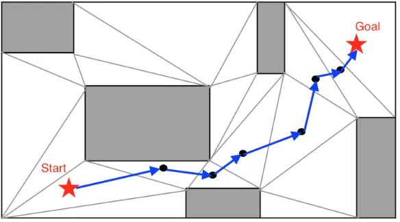
The third one is the grid graph (Fig.3), which is the most popular one to be used in
research. Grid-based pathfinding is required in many video games and virtual worlds
to move agents [14]. Grid graphs are made up by a collection of tiles. Each tile is
regarded as a node in the graph, and it can be set as a traversable or non-traversable
(obstacles) tile. Within different environments, the tiles could be in various shapes,
such as square grid (Fig.4), triangular grid (Fig.5), and hexagonal grid (Fig.6).
Com-pared with waypoint and navigation mesh graphs, we can observe that grid graphs
contain both the walkable and obstacles information of the environment, while the
other two graphs only refer to traversable areas, which means that grid graphs include
the entire game environment and even the environment changes; it will not charge
1. INTRODUCTION
Fig. 4: Square Grid Fig. 5: Triangular Grid Fig. 6: Hexagonal Grid
non-traversable. Additionally, the gird-based graph can be generated relatively faster
and it is widely used in a lot of pathfinding researches due to its simple block-like
structure.
We did the research based on the squared-grid graphs as it is used most widely
by games. Besides, it is easier to implement in the experiment and more obvious to
see the experimental result.
1.2.3
Heuristic
The heuristic function is designed for solving problems with a better performance
compared with classic methods: the outcome of the heuristic function is supposed
to be more quick, more optimal, or shorter than original results; however, it may or
may not end up with a better solution [15]. In pathfinding, the heuristic can decide
which direction to explore at each searching step using some given information. In
traditional search problems, heuristic means the estimation of the lowest cost between
any node n to the destination node, and it is usually represented as h(n); it is a quick
way to estimate how close the agent is to the goal.
To calculate the cost of two nodes, generally, three heuristic functions are used:
they are Manhattan distance, Octile distance and Euclidean distance,
respective-ly. Suppose we have two points, p1(x1,y1) and p2(x2,y2), the way to calculate the
distance between these two nodes with different heuristic functions is shown in the
1. INTRODUCTION
Fig. 7: Manhattan Heuristic Fig. 8: Octile Heuristic
Manhattan Distance
Manhattan distance is the distance between two points in which path is strictly
vertical or horizontal to the axes (see the path from Fig.7) [20]. The distance is
formed by the sum of grid lines between the two nodes, and we can get the distance
by the following formula:
h(p1, p2)M anhattan=|x1−x2|+|y1−y2| (1)
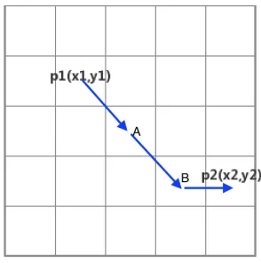
Octile Distance
Octile distance is the extension of Manhattan distance, which allows diagonal moves
on a squared-grid graph [2]. In Fig.8, the agent can walk diagonally from p1 to A,
from A to B, and then move horizontally to p2. This path is shorter than the final
path in Fig.7 since in Manhattan distance, it takes two units cost from p1 to A (two
steps) while in Octile distance only √2 units cost are used (one step), and it is the same process from point A to point B. Therefore, it can be concluded that when the
agent is allowed to walk diagonally, we can get a shorter solution path. The following
formula could calculate the Octile distance:
h(p1, p2)Octile = max((x1−x2),(y1−y2)) + (
√
2−1)∗min((x1−x2),(y1−y2)) (2)
1. INTRODUCTION
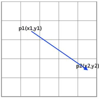
Euclidean Distance
Euclidean distance is the straight-line distance between two points, which means when
there is no obstacle on the path, the agent can move directly from the start point to
the end point without any turns (Fig.9). In this way, the length of the path is shorter
than the Manhattan distance and Octile distance (triangle inequality theorem). The
following formula can determine Euclidean distance:
h(p1, p2)Euclidean =
p
(x1−x2)2+ (y1−y2)2 (3)
Fig. 9: Euclidean Heuristic
Summary
From the above description of different heuristic functions, it can be observed that
when the agent is only allowed to walk vertically or horizontally, i.e., move to east,
south, west and north (four directions only), Manhattan heuristic could be the best
choice to estimate the distance to the goal; based on walking vertically and
horizon-tally, Octile heuristic could perform best when the agent can also move diagonally,
i.e., the agent is permitted to move to east, south, west, north, northwest, northeast,
southwest, southeast (eight directions). As for Euclidean distance, from Fig.9 we can
observe that there is no limit for moving directions since it calculates the direct
1. INTRODUCTION
path. However, there is no fixed heuristic function for the agent based on moving
directions. For instance, Euclidean heuristic also could be used when the agent is
au-thorized to walk in four directions only, but as the agent can only move in vertical or
horizontal directions, the actual cost (distance) should be longer than the estimated
distance by Euclidean heuristic.
1.3
Search Algorithms
There are many search algorithms for solving pathfinding problem, though they can
usually be classified under two categories: uninformed search and informed search.
Uninformed searches, also known as blind searches, refer to search algorithms that
only have knowledge of a start point and local connectively of the graph but have
no knowledge of the destination [7]. As a result, they usually traverse all possible
locations until reaching the target [7]. Breadth-first search and depth-first search
are the typical search algorithms in this type. In contrast, uninformed searches,
informed searches utilize local connectivity and some localized knowledge of the graph,
such as the location of its goal, the cost to travelling to the destination, to make
heuristic decisions during search [7]. In other words, informed searches do pathfinding
with some idea of how close the agent is to a given destination. This generates
more efficient results than uninformed search because the character does not expand
nodes that they know are not on the path to the target. In this classification, the
most typical algorithms are greedy search algorithm, Dijkstra’s algorithm [6] and A*
algorithm [10]. However, A* is the one used most widely in game applications and
has a great deal of optimized algorithms, such as Hierarchical A* [12], Windowed
Hierarchical Cooperative A* [21], IDA* (depth-first iterative-deeping A*) [13] and
EPEA* (Enhanced Partial Expansion A*) [9]. As A* is the most basic and popular
algorithm in research and real implementation, it is important to critically explore and
analyse how A* algorithm is used, and how to improve and maximize its application.
Therefore, we mainly worked on A* algorithm in this thesis , and it will be explained
1. INTRODUCTION
1.4
Properties of A* Algorithm
1.4.1
A* Algorithm
A* is one of the most effective and popular heuristic-guided algorithms used in
pathfinding. Given a certain Graph G(V, E) with a start node and a goal node,
A* has the ability to efficiently find an optimal path from the start node to the goal
node.
Searching from the given start point on the graph, A* builds a tree of all possible
paths that beginning from this start node, and every time, it expands one step further
on each path until it reaches the node on one of its paths that is the predetermined
goal node. To know the specific A* algorithm (Algorithm.1), several variants of A*
must first be understood. The process begins on start node, the agent will search the
graph and reach a node, which is represented by n. The distance between the start
node and n is g(n), while h(n) is a heuristic function that estimates the cost from
noden to the goal node. The sum of g(n) and h(n) is represented by f(n):
f(n) = g(n) +h(n) (4)
A* uses the f value (i.e., the total estimate cost of path through the node n) as the
evaluation to determine the node to be expanded in every step. Additionally, A*
maintains two sets to store the different nodes: theopen listand theclosed list. The
open list keeps track of nodes that are waiting to be examined in the future, while
the closed list stores nodes that have already been explored. To ascertain the entire
path lately, each node that has been expanded requires a pointer to its predecessors.
In Algorithm.1, A* uses a main loop to repeatedly gather nodes. Current is the
node with the lowest f value from the open list, if current is the target node, then
the path between it and start node must be found. It requires the agent to track the
predecessors from the final node until reach the node whose parent node is the start
node, then revises this path to map out the final path. However, if the current is
1. INTRODUCTION
list. Afterwards, A* generates all possible neighbor nodes tocurrent. If a neighbor is
already in theclosed list, it is discarded and the agent will move onto other neighbors.
if the neighbor is not in theclosed list, then the agent will verify whether it is in the
open list. If not, it will be added to the open list, and the agent will calculate the
f value of the node and set current as its predecessor. However, if the neighbor is
already in theopen list, the agent will calculate thef value of this node and compare
it with the duplicated node in the open list. If its f value is less than the duplicate,
it will replace the duplicate in the open list, and the agent will set its predecessor as
current before moving on. If its f value is equal to or greater than the duplicate, it
will be discarded directly and the duplicated one will be retained in the open list.
1.4.2
Optimality
The optimality of a solution may differ depending on the situation and could refer to
the fastest, shortest, or most efficient solution. In traditional pathfinding problems,
search algorithms are always expected to find an optimal path, which means the
closest between two nodes. In A*, the agent has to select the best possible optimal
nodes to keep on moving when it walks through several intermediate path. This
optimal choice allows the agent to achieve a high performance in the environment,
specifically the shortest path from the start to the goal node [18]. This solution is
called an optimal path.
1.4.3
Admissibility and Consistency
The use of an admissible heuristic function is critical to pathfinding when the goal
is to guarantee that the final solution is an optimal path [11]. In A*, the heuristic
is used to estimate the cost of reaching the goal node. An admissible heuristic in
A* means its estimated cost to the target node, represented as h(n), would never
exceed the actual cost it takes from the current location to the goal, represented as
h(n)∗. According to this requirement, h(n) <= h(n)∗ should always be true if we A*
1. INTRODUCTION
Algorithm 1 A* Algorithm
Input: A Graph G(V, E) with start node startand end node goal Output: Least cost path from start togoal
1: Initialize:
2: open list ={start}
3: closed list ={ }
4: g(start) = 0
5: f(start) = heuristic f unction(start, goal)
6: while open list is not empty do
7: current = the node inopen list having the lowestf value
8: if current = goal then
9: return “Path found”
10: end if
11: open list.delete(current)
12: closed list.insert(current)
13: for eachneighbour of current do
14: if neighbour in closed listthen
15: continue
16: end if
17: if neighbour not in open list then
18: open list.insert(neighbour)
19: end if
20: if g(current) + distance(current, neighbour) < g(neighbour) then
21: g(neighbour) = g(current) + distance(current, neighbour)
22: f(neighbour) = g(neighbour) + heuristic f unction(neighbour, goal)
23: neighbour.setParent(current)
24: end if
25: end for
26: end while
27: return “Path not found”
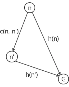
Apart from the requirement of admissibility, in A*, the heuristic function also
needs to be consistent to guarantee the optimality of a solution path [17]. Consistency
means the estimated cost (h(n)) to the goal is always less than or equal to the estimate
cost (h(n0)) from any neighbour of the current node to the goal plus the cost (c(n, n0))
from current location to this neighbour [29], i.e., it satisfies the triangle inequality
theorem (Fig.10):
h(n)≤c(n, n0) +h(n0) (5)
1. INTRODUCTION
Fig. 10: Consistency Diagram
the goal. From the evaluation function of A* that f(n) = g(n) + h(n), the function
for node n0 could be described as f(n0) = g(n0) + h(n0), which would provide an
induction as follows:
f(n0) = g(n0) +h(n0)
=g(n) +c(n, n0) +h(n0)
≥g(n) +h(n)
≥f(n)
(6)
The induction indicates that thef value of noden is always smaller than or equal
to the f value of its neighbours, which means that when examining the neighbour
node, n in the closed listwill never be updated again as itsf value is always smaller
than its neighbour’s. Thus, if the heuristic is consistent and if the exploring node
is discovered to already be in the closed list, A* algorithm moves on without doing
anything. A theorem can be gained through the consistency:
Theorem 1 If the heuristic is consistent, f value along any path is non-decreasing.
Theorem 1 is an important theorem as it will be used in the implementation. Since
there is no decrease of the f value on paths when the heuristic is consistent, it is not
1. INTRODUCTION
Additional, if the heuristic is admissible and consistent, another conclusion could
be obtained as:
Theorem 2 If the heuristic is admissible and consistent, A* could find an optimal
path [12].
The heuristic of Theorem 2 is admissible means that there exists the optimal path in
the environment sinceh(n) <= h(n)∗. For example, if the final actual cost from the
start to the goal isC∗, which is also the cost of the optimal path since the heuristic is
admissible, so we can conclude that A* only expands nodes whosefvalues are smaller
than or equal to C∗, and the f value of the last node on the path should be same as
the final optimal length. And as the heuristic is consistent, the f value of nodes on
paths in theclosed listwould never be changed. When combined with thef value of
the goal nodef(goal) = C∗, it can be proved that the solution path that A* finds is
the optimal one.
Our experiment only used admissible and consistent heuristics for the
implemen-tation of A*.
1.5
Thesis Contribution
The main cost of A* is the frequent insertion and deletion of the open list. Insertion
occurs when the algorithm is expanding neighbour nodes, as it needs to add those
neighbours with their information in theopen list. The deletion operation is required
in each step when moving the node with the lowest f value from the open list to
the closed list. Therefore, to enhance the efficiency of the A* algorithm during
pathfinding, it is critical to implement an open list in an efficient data structure so as
to increase the speed of the insertion and deletion operations. Typically, theopen list
of A* is implemented by a priority queue or min-heap to improve performance, which
takes O(log n) to carry out the insertion and deletion operations. However, this is
still very expensive when using A* on a large and complicated map with numerous
1. INTRODUCTION
The current study introduced a new data structure called multi-stack heap to
store the open list for A* algorithm based on 2D squared-grid map with Manhattan
distance, which only takes O(1) to insert and delete an element in the open list. It
is more efficient, especially when we have a considerable number of nodes to explore
comparing with other data structures. To address the frequent checking of duplicated
nodes in the open list before every insertion, another implementation method is
proposed: “Check From Closed List” method, which could save time from O(n) to
O(1). Moreover, the implementation of data structures was also optimized by using
the LIFO rule to select some nodes among nodes with the same f value to reduce the
number of nodes A* must explore.
1.6
Thesis Organization
This paper is divided in six sections. The first chapter offers an introduction and
describes the basic information of pathfinding and search algorithms with a particular
focus on the A* algorithm, which is principal component of the current study. The
second chapter reviews some typical data structures that host open lists for A* and
offers some analysis of their respective performances. The third chapter introduces
the current studys proposed data structure multi-stack heap in detail and provides
the theoretical analysis of the multi-stack heap. The fourth chapter describes a new
implementation of A* with respect to checking the duplicate nodes in the open list
before the insertion. The fifth chapter outlines the experimental setup, results, and
analysis. In this chapter, different data structures, such as the unsorted array and
the min-heap are implemented and compared with the multi-stack heap. The sixth
chapter offers a summation of the current studys key findings, while the seventh
CHAPTER 2
Literature Review
2.1
Operations of Open List
A* algorithm has two sets, open list and closed list, to store the nodes that are
waiting to be examined and nodes that have already been examined respectively.
There is a main loop that is utilized to repeatedly select the node with the lowest f
value from the open list, add it in the closed list, and insert its neighbours in the
open list until the agent finds its goal. The main cost of A* is the frequent insertion
and deletion operations associated with theopen list, and insertion operations of the
closed listas the heuristic is consistent. Thus, an efficient data structure for theopen
list is critical for the performance of A* algorithm.
There are four main operations of theopen list: “deleteMin”, “whetherContains”,
“insertNew” and “decreaseKey”. In each iteration, A* algorithm must find and
re-move the node with the smallestf value in theopen list (deleteMin). Once the agent
has removed the node from the open list, it explores all neighbours of the deleted
node, and insert them in the open list. Before the insertion, A* algorithm will verify
whether the inserting node is in the open list(whetherContains). If it is a new node
for the list, it is inserted into the open list (insertNew). However, if the node is
already in the list, and its f value is smaller than the one already in the open list,
then the duplicated node in the open list needs to be updated (decreaseKey). With
regard to updating the node in theopen list, there are normally two options. One
in-volves simply changing the information of the node in theopen list, more specifically,
2. LITERATURE REVIEW
involves discarding the repeated node in theopen listand adding this new node as a
replacement.
2.2
Data Structures
In the implementation, there are many choices of data structures for theopen list. The
most basic and simplest data structures are unsorted array, unsorted linked list, sorted
array, sorted link list. This series of data structures can be classified as the array.
The current study discusses the unsorted array and sorted array as representatives
as the array and introduces some other frequently-used data structures, such as the
hash table and min-heap [28]. In addition, the current study likewise analyses the
hot queue [4] for the use of the open list. The following discussion about the time
complexity is based on, having n nodes in the open list.
2.2.1
Array
For the unsorted array, insertNew is the most simple operation, which takes O(1).
However, deleteMin requires O(n) in order for the unsorted array to scan the array,
find the best node, and remove it. To verify whether the node is in the list, the
unsorted array also takes O(n). It needsO(n) to decreaseKey as A* has to scan the
open list first to find the duplicated node, but there is no other expense associated
with the updated node as the open list is unsorted.
As for the sorted array, the insertNew operation needs O(n) as the new node
should be put in the sorted order. Finding the best node and remove it is fast in
this data structure, which only takes O(1) since the array is already sorted and the
node with smallest f value is already at the end of the open list. As we can use the
binary search to check theopen list, which allows whetherContains to take O(log n)
to finish the job. For the decreaseKey, it needs O(log n) to find the node, and O(n)
2. LITERATURE REVIEW
2.2.2
Hash Table
In the hash table, sometimes it happens that when we apply a hash function to two
different keys, it generates the same index for both keys. However, those two items
cannot be located in the same address, this situation is called collisions of the hash
table [16]. To lower the collision probability, the hash table is usually set twice as big
asn. As every node has an individual key in hash table, normally, it only takesO(1)
to do the insertNew, whetherContains and decreaseKey. However, when the collision
occurs, the time complexity still depends, the worst case could be O(n). To find the
minimumf value from theopen list, the algorithm still needs to scan the whole hash
table, so that deleteMin takes O(n).
2.2.3
Min-Heap
The most typical implementation of the open list is the min-heap. Min-heap is a
complete binary tree, the value of each node on this tree is smaller than or equal to
its children’s values. In A*, the value indicates the f value. Min-heap is designed for
two basic operations, insert a new node and delete the node with the minimum value.
2. LITERATURE REVIEW
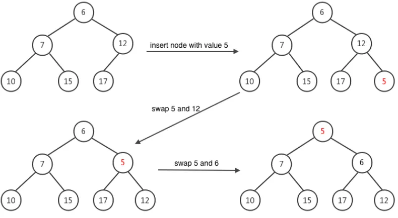
For the insertion (Fig.11), the new node is initially appended to the end of the
tree as the last leaf node. After that, repair the heap by comparing the value of
inserted element with its parent’s value, swap the position of the two nodes if the
added element has a smaller value, and keep the same process until the heap is a
min-heap (i.e., the value of each node on this tree is smaller than or equal to its
children’s values), this process is also named “bubble up”.
The smallest element can be found at the root of the heap, therefore, to delete
the minimum node, remove the root. After the deletion, move the last node from
the deepest level of the tree to the root position, compare the new root value with
its children, swap the position with the element with the smallest value and keep
comparing and swapping until the each node of this branch has a smaller value than
its children, another name of this process is “bubble down”.
Combined A* with the min-heap data structure, the insertNew and deleteMin
are same as the insert and delete operations of the min-heap respectively, which take
O(log n). For operating the whetherContains function, it is required to traverse the
whole open list, thus O(n) is needed. To decrease key on the heap, it takes O(n) to
find the element and O(log n) to repair the heap (as the updated element is always
with a smaller value, only bubble up is needed to repair the heap).
2.2.4
Hot Queue
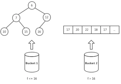
Hot queue, also called heap-on-top priority queue, is a combination of the multi-level
bucket data structure of Denardo and Fox [5] and a heap [4]. It is divided into k-level
buckets; the topmost bucket is a min-heap while the other buckets use the unsorted
array to store nodes. All buckets have a specific range. As for how to set thek value
and range of every bucket, the authors of the hot queue did not give a fixed function,
it depends on the specific circumstance.
Put theopen listin the hot queue, time for insertNew and deleteMin isO(log n/k)
in the top bucket which is same as the min-heap data structure. However, when the
inserted element is not in the range of the top bucket, then it takes O(1) to put in
2. LITERATURE REVIEW
within the unsorted array is converted into a min-heap, this process needs to be
completed in O(n/k). For the whetherContains, it still uses O(n) to scan the open
list. Decreasing key takes O(n) to find the element, if the element is in the topmost
bucket, it needs another O(log n/k) to decreaseKey on the heap, however, if it is in
the other bucket, there is no action needed to decrease the key.
Fig. 12: An Example Diagram of Hot Queue with 2 Buckets
Considering the fact of A* that not every node in the open list is necessarily
examined, we can take advantage of hot queue data structure as setting the hot
queue as a 2-level buckets, put nodes with small f value in the first level as a
min-heap, and put nodes with large f value in the second bucket as an unsorted array.
However, this is just a theoretical idea, in the real implementation, how to define the
2. LITERATURE REVIEW
2.3
Summary
From the above discussions about four operations of the open list and different
da-ta structures, we can compare the performance of each dada-ta structure with various
operations as Table.1.
Data Structures insertNew deleteMin whetherContains decreaseKey
Unsorted Array O(1) O(n) O(n) O(n)
Sorted Array O(n) O(1) O(log n) O(n) +O(log n)
Hash Table O(1) O(n) O(1) O(1)
Min-Heap O(log n) O(log n) O(n) O(n) +O(log n)
Hot Queue O(log n/k) O(log n/k) or O(n) O(n) +O(log n/k)
orO(1) O(n/k) or O(n)
Table 1: Time Complexity Comparison of Different Data Structures
It is hard to decide which data structure is the best since every data structure has
its advantages. For example, the unsorted array is good at insertNew while sorted
array performs well at deleteMin and whetherContains. Also, all data structures
per-form similarly with a small number of nodes in theopen list, i.e.,nis relatively small.
Considering whehtherContains must scan the whole open list (except for hash table
and sorted array, although hash table could also takeO(n) when collision happens) to
act operations; decreaseKey is a special case in pathfinding and it happens rarely, it
will not take a large portion of time even when it occurs sometimes. Therefore, for the
comparison, we focus on insertion and deletion. As we can see from the Table.1 that
the total time complexity of insertNew and deleteMin for the unsorted array, sorted
array and hash table isO(n), while the min-heap only needsO(log n) to perform the
operations. The hot queue may even better than the min-heap when it operates at
the topmost bucket, which only takes O(log n/k). However, when it precesses nodes
in other buckets, the maximum time complexity could be O(n/k), which could be
2. LITERATURE REVIEW
k when it compares with the min-heap.
As there are some uncertain factors of hot queue, we can confirm that it should
perform better than the Array series, but for the hash table and min-heap, it still
depends since hash table could take advantage of whetherContains and min-heap has
the possibility to be better than hot queue too, we do not consider the hot queue
in our later research. The performance of hash table is also unstable, if there is
no collision happens, it would be a more efficient data structures comparing with
Array definitely, and it also could be better than min-heap at whetherContains and
decreaseKey operations. But when collisions happen, it is hard to say which one is
better, therefore, the hash table is not in the final comparison of our research as well.
After reviewed and compared all those data structures, we regard the min-heap
as the most competitive data structure for the open list, which is the main data
CHAPTER 3
Multi-Stack Heap
3.1
Motivation
When we researched pathfinding problem, found that whether Single Agent or
Multi-Agent pathfinding, most of those searching algorithms are based on A*. For the
implementation of A*, there are several typical data structures to perform the open
list, while the open list is the most consuming part of A* algorithms, which are
already discussed in literature review section. Those data structures are pretty
ef-ficient to store the open list, and can be commonly used in different situations and
environment. However, we just found that grid maps have a structure that can be
exploited when we were trying to do some simple implementation of A* within
differ-ent maps. For the squared-grid graph, we have several observations when operating
the pathfinding with Manhattan distance.
Suppose we use Manhattan distance as the heuristic, and the agent is allowed to
walk only horizontally or vertically. Set the searching environment as Fig.13: white
cells are the traversable grids while black blocks indicate obstacles on the graph that
the agent cannot walk through; S and G means the start node and goal position of this
pathfinding problem; the map is set on a coordinate axis, so every node on the graph
can be represented by coordinate (x, y); the cost of every cell is 1, for calculating the
h anf value. In each cell, the number at the bottom left corner is the hvalue of this
node while the bottom right corner value is the f value, and the value at the top left
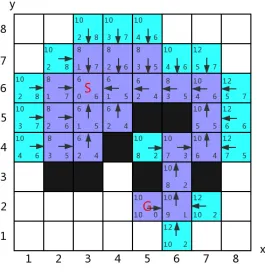
corner indicates thef value; additionally, there is an arrow points to its parent node.
3. MULTI-STACK HEAP
been put in theclosed list, blue background means the node is in the open list.
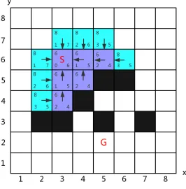
Fig. 13: An Example Environments for A* Pathfinding (all nodes with f value “6” have been explored)
In the Fig.13, nodes with f value “6” have been explored already and they are
removed from the open listto theclosed list. Currently, the open liststill has other
nodes, whosef values are “8”. The next step is still finding the node with the smallest
f value from the open list and examine it until we find the determined goal. As all
node in the open list with the same f value, the algorithm could pick one randomly
and keep going. For instance, the node (6,6) is the next one to be explored, firstly,
the algorithm checks whether it is contained in the closed list, which is not, then
removes it from the open list and inserts the node in the closed list. At the same
time, expanding its neighbours nodes (6,7), (7,6), (6,5) and (5,6) and calculating
their f value respectively (Fig.14). As the node (6,5) is an obstacle, it is discarded
without any operation. The node (5,6), whetherContains could find out that it is
3. MULTI-STACK HEAP
as well as theirf values are the same, it is not necessary to update it. Node (6,7)and
(7,6) are inserted in the open list as new nodes.
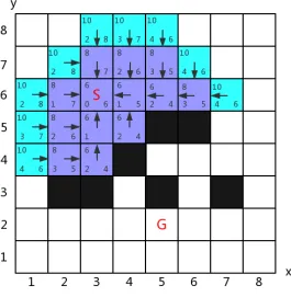
Fig. 14: An Example Environments for A* Pathfinding (all nodes with f value “8” have been explored)
In the Fig.14, it can be seen that all nodes with f value “8” have been explored
and the goal has not been found yet. Meanwhile, some nodes with newf value “10”
appear in the open list. Again, A* has to pick the node with minimum f value
again to do the examination until the agent reaches the target. Let’s say, we pick the
node (7,6), and expand its neighbours, we could found that a new f value “12” is
generated, (7,7) and (8,6) are inserted in the open list with f value “12” and (7,5)
is added with f value “10”. Repeat the exploring process until the goal is found like
the status in the Fig.15. And after reaching the goal, follow the pointer to the parent
of every node on the path until finding the start node, get the final path by revising
the pointer on this path from the start node to the goal node. The pathfinding task
3. MULTI-STACK HEAP
Fig. 15: An Example Environments for A* Pathfinding (find Goal and stop searching)
From the process of solving this pathfinding problem using A*, we have two
obser-vations: On a squared-grid graph, using Manhattan distance as the heuristic function
(only move in four directions), the f value of a node is always equal to or 2 less than
its children’s f value; there are at most 2 different kinds of f values in the open list
at the same time.
When A* is expanding children of the node nand inserting them in the open list,
the g value of those neighbour nodes should be 1 more than node n as the agent
walks 1 step further. However,g value could be different. If the agent is walking in a
correct direction, i.e., moving toward the goal, then theg value of this child should be
1 less than node n. Therefore, compared ton, children nodes’ g values are 1 bigger,
h values are 1 smaller, so that
3. MULTI-STACK HEAP
this equation is proved. Take the Fig.15 as an example, whether the node (3,5) or
(5,6), comparing to their parent node, they are always 1 step closer to the G than
their predecessors, this is the reason that they have the same f value as their parent.
Nonetheless, when the expanded neighbour node is located backward (relative to its
parent noden) to the destination, thehvalue of this child should be 1 larger, because
it makes the agent 1 step further to the destination. This happens a lot when the
agent wants to avoid obstacles. Check the node (5,6) in the Fig.15, to reach the
destination in a most efficient way, it should move to (6,5), but as this node is an
obstacle, and there is no other choice to get closer to the target node, the agent has
to avoid this obstacle to reach the goal by moving to (6,6). Node (6,6) is at the
opposite direction to the destination node by walking through (5,6). As both g and
h values decrease 1 separately, f value of this child node could be 2 more than the
noden. We can get
f(n.children)−f(n) = 2 (2)
which is correct as well in the specific case. Therefore, the first observation is true.
As for the second observation, primarily, we know that A* always explores the
node with the lowest f value from the open list. Starting from the start node, it
only inserts neighbours of the examining node in the open list, combined with the
first observation thatf value of parent node is whether equal to or 2 smaller than its
neighbours, there are at most two different kinds of f values in the open list, and if
there are two variousfvalues, they should differ in 2. Whenf(n.children)−f(n) = 2, nodes with f value “f(n.children)” would never be picked until all nodes with “f(n)”
f values are removed from the open list. After that, there is no node with f value
“f(n)” in the open list, nodes with “f(n.children)” as f value are examined. At this
time, those nodes’ neighbours could appear in the open list, but that is fine as there
are only nodes with f value “f(n.children)” in the list, and their neighbours’ f values
are at most 2 bigger than “f(n.children)”, there are still only two different types off
in the open list. When f(n) = f(n.children), A* could pick any node from the open
3. MULTI-STACK HEAP
its neighbours f value must equal to or 2 larger than “f(n)”, which still meets the
second observation. We also can observe it from our example implementation on
Fig.13, Fig.14 and Fig.15, when the open list still has some nodes with “6” f value,
the other f values it inserted are only “8”. Only when all nodes with f value “6”
have been removed from the open list, it begins to expand nodes with f value “8”,
and some “10” as f value exist in the list. Therefore, we can conclude that in the
open list, it always has one or two different f values at the same time, which means
the second observation is a truth too.
Getting some inspirations from the idea of multi-level bucket data structure, for
the open list, we decide to put nodes with same f value in one bucket and based
on our observations, at most two buckets are required in this new data structure.
Even though A* has to find the smallestf value between buckets, there are at most
2 different values, finding the smaller one between two values is not expensive in
any way. However, we prefer to build some connections between buckets, especially
when we want to extend our limit from Manhattan distance to some other heuristic
functions (more than 2 buckets). Considering when there are 2 more buckets, the
most expensive operation should be finding the bucket with the smallest f value, we
thought of the idea from the binary search. Therefore, we build our data structure
based on min-heap, every bucket is regarded as a node on the heap.
3.2
Multi-Stack Heap
3.2.1
Data Structure of Multi-Stack Heap
Multi-stack heap is a data structure that built on a binary tree. However, every
“node” on the tree is a stack which contains nodes with the same value, and we
called this node container as stack node. Similar with min-heap, the value of each
stack node is larger than or equal to its parent stack node, Check the Fig.16, the
nodes n1, n2 and n3 in every stack have the same value and v1, v2, v3 ... indicate
3. MULTI-STACK HEAP
≤ v3, similarly, v2≤ v4 and v2 ≤ v5,v3 ≤ v6 and v3 ≤v7 and so on.
Fig. 16: Data Structure of Multi-Stack Heap
3.2.2
Operations of Multi-Stack Heap
The four main operations of this data structure were analysed as other data
struc-tures discussed in chapter two, which are insertNew, deleteMin, whetherContains and
decreaseKey. The following explanation of the multi-stack heap is based on that we
have k stack nodes on the heap, and n is the total number of nodes that stored on
the heap, i.e., the summation of nodes from each stack node (n ≥ k).
insertNew
For the insertion, check the value of this new node on the heap whether the heap
contains this value, if it is, insert this node at the end of the found stack and done,
this process takes O(k). For example, in Fig.17, if we want to insert a node with
value 8, then we need to find the stack whose value is 8, and then add the new node
at the end of the stack (i.e., append after n4). Otherwise, create a new stack, push
the new node in this stack, append the new stack at the end of the heap as the last
leaf and set value of this stack as the value of the inserted node, comparing with value
of its parent stack and swap positions of those two stacks if its values is less than
its parent stack, do the same comparison until we do not move the new stack. This
process is same as the “bubble up” of the min-heap, we call it “bubble up” in the
3. MULTI-STACK HEAP
on the heap takes O(k). Therefore, it takes O(k) + O(log k) to insert a new node if
its value is not stored previously on the heap. Take structure in Fig.17 as an example
again, when we want to insert a new node n12 with value 5, check whether its value
is on the heap, and the result is not, then build a new stack and push inn12 like the
top heap on Fig.18; after that, compare 5 with 10, 5 is smaller, swap their positions;
compare 5 with 6 and swap positions of 5 and 6 again since 5 is still the smaller one;
there is no parent stack of 5 as stack with value 5 is the root stack now, the task is
completed and the final status of this multi-stack heap should be same as the bottom
heap on the Fig18.
Fig. 17: A Specific Example of Multi-Stack Heap Structure
deleteMin
To delete the node with the smallest value, it could take O(1) or O(log k). As the
topmost stack on the heap always contains nodes with the minimum value, deleting
the minimum one is deleting one from this stack randomly. If the stack has more
than one node, just leave the stack and the job is finished, this is the condition it
needsO(1). However, after the deletion, if the stack is empty, i.e., the deleted node is
the last node in this stack, a bubble down is needed as min-heap. Firstly, delete the
empty stack and put the last leaf stack from the heap at the root position, compare
new root’s value with its child stacks, swap position with the smaller child stack if its
value its greater than one of its child stack or both of left and right stack. This is why
3. MULTI-STACK HEAP
Fig. 18: An Example of Multi-Stack Heap Insertion based on Fig.17 (a new node whose value is not contained on the multi-stack heap)
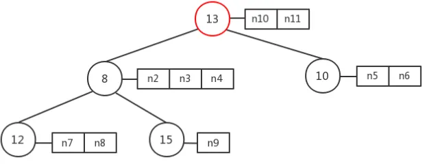
Fig. 19: An Example of Multi-Stack Heap Deletion based on Fig.17 (move the last leaf stack as the root of the heap)
is to delete the node with minimum value on Fig.17 now. As n1 is the only node
in the top stack, after the deletion, the stack is empty. The first step is to remove
the empty stack, move the last stack on the heap, the stack with value 13, to the
root position as Fig.19; compare 13 with its children 8 and 10, 8 is the smallest one,
3. MULTI-STACK HEAP
Fig. 20: An Example of Multi-Stack Heap Deletion based on Fig.17 (the final status after the deletion)
of its new child stacks, which are 12 and 15 respectively, 12 is the minimum one so
swap 13 and 12, the mission is completed as there is no other child stack of 13, the
ultimate heap should be as the multi-stack heap in Fig.20.
whetherContains
As we know, the operation whetherContains is to check whether the data structure
contains the checking node. As nodes stored in the multi-stack heap are not only
with “value” attribute, it probably has some other attributes such as a pointer to its
predecessor, or the specific location of this node on a graph. The property “value” is
the metric that we used to store nodes in the structure. Therefore, whetherContains
in multi-stack means to check whether the checking node is already inserted on the
heap, the value of inserting node contained on the heap is not used as the value could
be changed. We have to identify whether two nodes are the same node by comparing
their constant attributes such as a specific coordinate or an exclusive name that stored
on the heap. The specific whetherContains process is shown in the following example:
check whether the node n3 is on the multi-stack heap based on Fig.17. Suppose the
name of each node is exclusive, i.e., the name “n1” is the specialised name for this
node, if another node also with name “n1”, they must be the same node. As we
already know all information of this node before doing the check, to check whether
3. MULTI-STACK HEAP
compare names of nodes in each stack to find one with name “n3”. In this example,
a node with the name “n3” is detected in the left child of the root stack, so we can
return the result that this multi-stack heap is already contained node n3. However,
if the question is checking whether the heap from the Fig.17 contains noden15, then
the answer should be negative after scanning the whole tree. whetherContains needs
O(n) to get the result.
decreaseKey
decreaseKey means updating information of a node which is already contained in the
data structure, and the value of this node is changing to smaller than before. On the
multi-stack heap, find the node that is already on the tree needsO(n) (same with the
operation of whetherContains). Next step is to update the information of the found
node. As the node’s value is changed, it should be relocated at some other stack.
Relocating process is the same as inserting a new node on the heap. Whether the
changed value is already on the heap is being checked first, if the stack with the same
value is found, move this node from the old location to this stack, put it at the end;
otherwise, create a new stack, put the node in the stack, append the new stack at the
end of the multi-stack heap and bubble up until the heap meets the requirement of a
multi-stack heap. Compared to other operations, decreaseKey is expensive as it takes
the time to do the whetherContains first and then do the operation of insertNew.
Summary
From the analysis of the four operations, we can see that the time complexity really
depends onk, i.e., the number of stacks. Whenkis far smaller than the total number
of nodes on the multi-stack heap n, which means that there are a large number of
nodes with the same value stored in one stack, this data structure could be very
efficient compared with the data structures discussed in the second chapter, such as
the array, min-heap. However, when there are few nodes in each stack, k is very
close to n, in this case, comparing with other data structures, the advantage of the
3. MULTI-STACK HEAP
duplicated value on the heap, every stack contains one node, then the multi-stack
heap is same as the min-heap structure and time complexity of operations should be
the same as the min-heap as well.
3.3
Multi-Stack Heap for A*
In A*, implementing multi-stack heap as theopen list, for every node, the f value is
stored as the value on the heap. Therefore, each stack contains nodes with same f
value from the open list and the f value of nodes stored in the stack node is equal
to or greater than the f value of nodes in its parent stack node as the feature of the
multi-stack heap.
Combined the observations we obtained based on a square-grid graph using
Man-hattan heuristic with the data structure of multi-stack heap, there are at most 2
stacks on the heap as there are at most 2 different f values in the open list at the
same time (k = 2). And when there are two stacks on the multi-stack heap, their f
values must differ in 2.
3.3.1
A Pathfinding Case
To illustrate the detailed functions of multi-stack in A*, we set a pathfinding
environ-ment as Fig.21 (the initial status of the environenviron-ment from Fig.13), and the multi-stack
heap is performed as the open list in the whole solving process. On the graph, S is
the start node whileG is the goal node, black cells mean obstacles, every node could
be represented as the coordinate (x, y) and the cost to pass a traversable cell is 1.
A* begins to search from the start location S and initially there is only S in the
open list, therefore, the multi-stack heap only has one stack with one node S(3,6)
stored in this stack. The next step is to explore the nodeS and move it to the closed
list. Meanwhile, expand its neighbours (3,5), (4,6), (3,7) and (2,6) and calculate
theirf values respectively. Get those nodes’ information as Table.2 and put the nodes
in theopen listseparately. Before the insertNew operation, we need to check whether
3. MULTI-STACK HEAP
the answer is no, then begin to insert. Check the insertion process from the Fig.22,
(a) creates new stack with f value 6 and node (3,5) is inserted in this stack; the f
value of (4,6) is still 6, append it after (3,5) as (b); in (c), the algorithm builds a
child stack as (2,6) hasf value 8, which is not contained on the heap; (d) shows the
node (4,6) is inserted after (3,7) as its value is also 8.
Fig. 21: An Example Pathfinding Environment
Neighbour Nodes f Value Parent Node
(3,5) 6 (3,6)
(4,6) 6 (3,6)
(3,7) 8 (3,6)
(2,6) 8 (3,6)
3. MULTI-STACK HEAP
Fig. 22: Insert Neighbour Nodes ofS on Multi-Stack Heap
In the next loop, A* has to find the node with minimum f value from the open
list and move it to the closed list (deleteMin). Thus, we pick a random node from
the root stack of the heap, for instance, we select node(4,6) on Fig.22 (d), delete it
and get the multi-stack heap as Fig.23 (a). After the deletion, the node(3,5) is still
in the stack, which is not empty so that we can just leave it and continue the next
step. Expand neighbours of (4,6) and get the information as Table.3.
Neighbour Nodes f Value Parent Node
(4,5) 6 (4,6)
(5,6) 6 (4,6)
(4,7) 8 (4,6)
(3,6) 8 none
Table 3: Information of node(4,6) Neighbour Nodes
Same as the insertNew operation in the last loop, the result of whetherContains
for node (4,5) is negative so it can be inserted on the heap directly. As the f value of
(4,5) is 6, it is added at the end of the root stack (Fig.23 (b)). Node(5,6) and (4,7)
3. MULTI-STACK HEAP
f values are 6 and 8. For the node(3,6), when we checked the closed list and found
that it is already stored in the closed list, so we skip this neighbour node and keep
going... Do the same process until we find the exploring node is the G(5,2).
Fig. 23: Insert Neighbour Nodes of (4,6) on Multi-Stack Heap
3.3.2
Operations Analysis
The agent is only allowed to walk in four directions on a squared-grid graph with
Manhattan heuristic, take advantages of this, implementing the open list with the
multi-stack heap could be much more efficient.
insertNew
When inserting the new member on the multi-stack heap, there are two conditions.
One is that the f value of the inserting node is already on the heap, then we need to
find the stack whose value is same as this node and add it at the end of the stack.
As there are at most two stacks on the heap, finding the specific stack between one
or two takes O(1). Another condition is that a new stack has to be created for the
inserting node when there is no same f value stored on the heap, then we need to
3. MULTI-STACK HEAP
up this multi-stack heap. Since there are at most two stacks on the heap at the same
time, if we need to create a new stack, there must be just one stack on the heap
before we append the new stack. Therefore, bubble up the heap between two nodes
also takes O(1). As a result, insertNew in multi-stack heap takes O(1).
deleteMin
Nodes with the smallest f value are always stored on the root stack of the
multi-stack heap, therefore, to delete the minimum one, go to the top multi-stack and pick one
randomly to remove, which needs O(1) to do it. After the deletion, if the stack is
empty, and there are two stacks on the multi-stack heap at this time, then we delete
this stack and put another stack as the root; if the empty stack is the only stack
on the heap, and there is no neighbour node to insert in the open list, then the
pathfinding is terminated as there is no path found. Therefore, it can be concluded
that the deleteMin operation takes O(1) to delete the node with minimum value on
the multi-stack heap.
whetherContains
Before inserting a node on the heap, we have to check whether this node is contained
in the closed list. As there are not many operations and cost of the closed list, the
same data structure (normally, an array) is used for theclosed listin different
imple-mentations, so that the operation of the closed list is not calculated and compared.
The whetherContains means the operation to check whether the multi-stack heap
already contains the inserting member on the open list. Thef value of the checking
node could be different with the same node that is already stored on the heap (if
the f value of checking node is smaller, then we need to decreaseKey). Hence, in
our indicated background, as there is other information of nodes stored on the heap,
to check whether the two nodes are identical, we compare coordinates of nodes by
scanning the whole multi-stack heap. Return to a positive result if found the two
n-odes with the same coordinate. Therefore, similar with most of other data structures,