Development of patient specific cardiovascular models predicting dynamics in response to orthostatic stress challenges

Development of patient specific

cardiovascular models predicting dynamics

in response to orthostatic stress challenges

Johnny T. Ottesen, Vera Novak, Mette S. Olufsen

Department of Science, Systems and Models

Roskilde University,

4000 Roskilde, Denmark

Division of Gerontology

Beth Israel Deaconess Medical School and Harvard University

Boston, MA 02215

Center for Research in Scientific Computing and Department of Mathematics

North Carolina State University, Raleigh, NC 27695

Abstract

Physiological realistic models of the controlled cardiovascular system are constructed and validated against clinical data. Special attention is paid to the control of blood pressure, cerebral blood flow velocity, and heart rate during postural challenges, including sit-to-stand and head-up tilt. This study describes development of patient specific models, and how sensitivity analysis and nonlinear optimization methods can be used to predict patient specific characteristics when analyzed using experimental data. Finally, we discuss how a given model can be used to understand physiological changes between groups of individuals and how to use modeling to identify biomark-ers.

1

Introduction

50 55 60 65 70 75 80 85 90 40

60 80 100 120 140 160

time [sec]

pressure [mmHg]

50 55 60 65 70 75 80 85 90

60 80 100 120 140 160 180

time [sec]

pressure [mmHg]

Figure 1: Blood pressure [mmHg] versus time [sec] during STS for a healthy young (left) and a hypertensive elderly (right) subject.

50 55 60 65 70 75 80 85 90

0 20 40 60 80 100 120 140

time [sec]

blood flow velocity [cm/sec]

50 55 60 65 70 75 80 85 90

0 10 20 30 40 50 60 70 80

time [sec]

blood flow velocity [cm/sec]

50 60 70 80 90 40 50 60 70 80 90 100 time [sec] HR [bpm ] Model Data baseline firing Vestibulo-sympathetic activation parasympathetic withdrawal sympathetic activation standing relaxation initial blood pressure decrease

50 60 70 80 90

40 50 60 70 80 90 100 time [sec] HR [bpm ] Model Data baseline firing initial blood presure decrease parasympathetic withdrawal sympathetic activation Vestibulo-sympathetic activation relaxation standing

50 60 70 80 90

40 50 60 70 80 90 100 time [sec] HR [bpm ] Model Data baseline firing initial blood pressure decrease Vestibulo-sympathetic activation parasympathetic withdrawal sympathetic activation relaxation standing

Figure 3: Heart rate [bpm] versus time [sec] for a healthy young (left), a healthy elderly (middle) and a hypertensive elderly (right) subject.

The baroreflex regulation acts through stimulation of baroreceptors located in the carotid and aortic walls. These receptors are stretch receptors, which sense changes in arterial blood pressure. A blood pressure drop leads to decreased fir-ing of the afferent baroreceptor nerves, which gives rise to parasympathetic with-drawal and sympathetic activation. Parasympathetic withwith-drawal induces a fast increase in heart rate within 1-2 cardiac cycles, while sympathetic stimulation yields a delayed (within 6-8 cardiac cycles) increase in vascular tone (resistance and compliance), cardiac contractility, and a further increase in heart rate [38, 8]. At the same time cerebrovascular tone is modulated through metabolic vasoreg-ulation (mediated by changes in CO2) and myogenic autoregulation (regulation responding to local changes in blood pressure). It is not clear if autonomic control also regulates cerebrovascular tone. Some recent studies [45, 46] have indicated that cerebral vascular tone is modulated by stimulation of cholinergic nerves ter-minating in the cerebral vasculature.

from the brain to the heart, which for a period of time may increase right atrial pressure stimulating pulmonary baroreceptors, which has potential to lower heart rate. During STS, there is no hydrostatic change between various regions in upper corpus, thus all pooling of blood will be in the legs. Therefore this motion does not give rise to the immediate decrease in heart rate upon standing.

Another difference is that HUT is almost entirely passive, while STS require muscle contraction in the legs activating muscle sympathetic nerves (MSNA), which may increase heart rate before the observed drop in blood pressure. Other explanation for the initial increase in heart rate include stimulation by the vestibu-lar system, and/or by central command.

During HUT and STS experiments typical cardiovascular measurements in-clude: arterial blood pressure, heart rate, and cerebral blood fow velocity mea-sured using Transcranial Doppler ultrasound. These measurements are then used to assess short term autonomic (baroreflex) and cerebral autoregulation. Most common data analysis methods use some form of linear response models. For example, baroreflex sensitivity [36, 9] is often assessed using spectral transfer functions relating changes in systolic blood pressure to interbeat intervals. Prob-lems with this method is two-fold; first the method is linear, second it is limited to analysis of the relationships between two signals. Another limitation is that these methods lack the ability to predict how changes in neural responses interact to maintain arterial blood pressure.

those that do have potential to serve as biomarkers characterizing varying states of diseases. Finally, we show dynamics observed during longer time scales (>35 min) for a subject who experienced syncope. Note, at the onset of syncope blood pressure and heart rate decreases rapidly. We show (see Fig. 15) that our model is able predict a similar behavior for a suitable choice of parameters, i.e., when saturation in the vascular tone is reached.

2

Methods

2.1

Experimental design

The results reviewed used STS and HUT data from a number of healthy, hyper-tensive, and elderly subjects. The healthy young and elderly subjects where not treated for any systemic disease and the hypertensive elderly subjects were diag-nosed and treated for hypertension but had no history of more than one episode of syncope. Subjects with a history of diabetes, stroke and brain injury, renal liver and other systemic disorder were excluded. Instrumentation for all studies was done using similar protocols. Heart rate is measured using a three-lead electrocar-diogram (ECG) (SpaceLab Medical Inc., Issaquah, WA). A transcranial Doppler system (MultiDop X4, DWL Neuroscan Inc. Sterling VA) was used to obtain con-tinuous measurements of blood flow velocity in the middle cerebral artery. The data was acquired by insonating the artery through the temporal windows using a 2-MHz pulsed Doppler probe. The probe was positioned to record the maximal flow velocities and stabilized using a three-dimensional head frame positioning system. A photoplethysmographic device mounted on the middle finger of the non-dominant hand was used to obtain non-invasive beat-to-beat blood pressure (Finapres device, Ohmeda Monitoring Systems, Englewood, Colorado). To elim-inate effects of gravity, the hand was held at the level of the right atrium and supported by a sling. All physiological signals were digitized at 500 Hz using Labview NINDAQ software (National Instruments, Austin, TX) and stored for offline analysis. Before data were analyzed they were down-sampled to 50 Hz.

• STS protocol: After instrumentation, subjects sat in a straight-backed chair with their legs elevated at 90◦

in front of them. After five minutes of stable recordings, the subjects were asked to stand up. Standing was defined as the moment both feet touched the floor, recorded by a force platform.

10 minutes. After resting in this position, the table was then tilted to 70◦

for 10 minutes.

• Syncope protocol: Using the HUT protocol described above the subjects were tilted to 70◦

from supine to upright position and then kept upright until presyncope (>35 min) at this time the subjects were returned to supine position, and the subjects regained consciousness immediately

The STS and the open loop model data analyzed were collected from Lewis A. Lipsitz and Vera Novaks laboratories at Hebrew Senior Life and at the Beth Israel Deaconess Medical Center, Boston, MA. All subjects provided informed consent approved by the Institutional Review Board at Hebrew Senior Life and at the Beth Israel Deaconess Medical Center. HUT data used for the syncope study was obtained by Jesper Mehlsen, Medical Director, Department of Physiology and Nuclear Medicine, Frederiksberg Hospital, University of Copenhagen, Denmark.

2.2

Modeling strategy

The following protocol provides an outline of the methodology that has guided our work with the development of patient specific models.

• Data, knowledge and structure: Development of reliable patient specific physiological models require detailed knowledge of the underlying biologi-cal system combined with a clear definition of the outcomes that the model is supposed to predict or prescribe. Sufficient insight into both the physiol-ogy and available modeling techniques is crucial. In this spirit, structures in the data analyzed in this study were revealed using standard statistical tools combined with nonlinear optimization. Results of these analysis lead to knowledge of the system revealed through collaboration between math-ematicians and physicians. Other methodologies that can be used for ana-lyzing the structure of the system include filtering and generalized principal component analysis.

conservation laws) whenever possible and the parameters shall have a phys-iological interpretation. Such models are denoted canonical models. The models discussed in this review were developed to study patient specific short-term regulation of heart rate, blood pressure, and cerebral blood flow velocity during STS and HUT. The models were formulated as dynamical systems. Steady state analysis of the model equations were considered. Af-terward models were used for analysis of baseline dynamic behavior and later coupled with control models allowing prediction of dynamics during the orthostatic challenges (STS and HUT).

• Parameter identification and estimation: The main goal with the models presented here [27, 28, 30, 21, 20, 22, 3, 31, 5, 2] was to identify biomarkers (model parameters) that allow the models to display the dynamic behavior observed in the data. Estimation of these quantities requires solution of an inverse problem, where a set of parameters is estimated that minimize the error between measured and computed quantities. For example, in the open loop heart rate model, a set of parameters minimizing the least squares error between computed and measured values of heart rate was identified, and in the closed loop model we minimized the least squares error between computed and measured values of blood flow velocity and arterial blood pressure.

For a given model and a given set of data, it is likely that the model is in-sensitive to a subset of the model parameters, i.e., changes in that subset of parameters has a negligible impact on the solution. This set of parameters is called insensitive, and such parameters cannot be estimated via solution to the inverse problem. Second, among the subset of parameters that are sensitive it is likely that parameters are correlated. For example, two resis-tors in series could both be sensitive, but it is not possible to identify both resistors separately, knowing only the total potential drop and current, e.g.,

es-timated using literature data coupled with anthropometric (height, weight, age, gender) information, allometric scaling relations, as well as mean and steady state values extracted from the data.

• Optimization algorithms: To perform the required parameter estimations non-linear optimization algorithms was used. Two methods were used, gra-dient free methods: the Nelder-Mead method (a simplex method) [18, 20, 21, 22], genetic algorithms [7], and implicit filtering [7]; and gradient-based methods: Newtons method and the Levenberg-Marquardt method [31, 5]. The advantage of gradient-based methods is that sensitivities are computed as part of the optimization. A disadvantage of these methods is that the ODEs should be differentiated with respect to each of the parameters. Other methods that have received much attention recently include Kalman filter-ing [3], particle filters, functional differential analysis, and sequential Monte Carlo (SMC) methods.

• Validation of models: The process of solving the inverse problem estimat-ing parameters that allow the models to predict data is one aspect of model validation, but this type of analysis should be combined with more general validation methods. For example, once a set of parameters have been esti-mated using one dataset, the models should be validated using other datasets not used for the parameter estimation. However, this type of validation often cannot be used for biological systems where inter and intra variations within and between groups of individuals are large. One way to validate such mod-els is to use K-fold cross-validation [13] where a subset within one data-set is used for prediction of model parameters, while the remaining data are used for validation. Other validation methodologies include model reduc-tion (discussed in [6]) and analysis of sub-mechanisms. Common for all of these validation methods is that if a model fails to be validated it should be adjusted. This process of iterative model development often generates important new insights into the underlying physiology [12, 1, 40, 30].

can provide insight into quantities that cannot directly be measured exper-imentally. Examples include estimation of cerebrovascular resistance [17, 31], delay in baroreflex firing rate, baroreflex dampening, and baroreflex gain [21, 22]. To determine if biomarkers differ significantly between groups of subjects, and if biomarkers can be used to identify variant causes of a given illness statistical tests can be performed. For example, in a recent study [31] we showed that cerebrovascular resistance is increased with ag-ing.

• Multiscale models: Frequently models contain several scales, one could have an overall system level model predicting overall pressure level cou-pled with a detailed 3D model describing wave propagation and blood flow dynamics in a given artery. Coupling of such models have received much at-tention recently, and it is important when models are coupled that the overall dynamics is preserved. For example if a given biomarker has been identified from a system level model, if modeled correctly, the detailed model should serve to refine prediction of the biomarker.

We emphasize that the variant steps discussed above are not all independent, and should merely be considered as components important to assess in development of subject specific models. Overall, the main components included are: choice of model, parameter identification, parameter estimation, model validation, and comparison of outcomes (biomarkers) among study populations.

2.3

Mathematical models

rate model, we used blood pressure data as an input to predict heart rate and the links made visible through the model include baroreflex firing rate, sympathetic and parasympathetic tone, and concentrations of acetylcholine and noradrenaline, and for the closed loop model quantities predicted include cerebrovascular resis-tance, cerebral and systemic blood pressure. These model based quantities can be used to form hypotheses for how these ”invisible” quantities may vary, and with more experiments, it may be possible to validate the various sub-models. Thus, with sufficient validation, we may view the model together with the outcomes as a method that can provide insight into an individuals control system like a fin-gerprint. Such biomarkers have potential to be relevant for treatment of several diseases such as hypertension, see [20, 18].

2.3.1 Open loop model

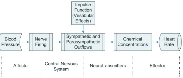
The overall function of the baroreceptor feedback mechanism is known. However, the underlying biochemical mechanistic processes are not fully understood and are difficult to investigate in-vivo. In the studies summarized here we used STS and HUT experiments to investigate the short-term baroreceptor feedback regulation of heart rate, detailed description of the model can be found in [24, 25, 30, 21, 22]. To investigate baroreflex regulation of heart rate we developed the model shown in Fig. 4. This model uses blood pressure as an input to predict heart rate using the following five steps:

• Mean blood pressure is used to predict afferent baroreflex firing rate. • Sympathetic and parasympathetic outflows are computed from the

barore-flex firing rate combined with stimulation by muscle sympathetic nerves, the vestibular system, and from central command.

• Concentrations of acetylcholine and noradrenaline are computed as func-tions of the sympathetic and parasympathetic outflow.

• Heart rate potential is computed from chemical concentrations. • Heart rate is predicted from the heart rate potential.

The baroreflex model uses weighted mean blood pressure as an input to predict the afferent firing rate using a nonlinear differential equation of the form

dni

dt = ki

dp dt

n(M ₋n)

(M/2)2 −

ni

τi

, i=S, I, L (1)

Figure 4: Elements of the baroreceptor feedback chain controlling heart rate.

whereni [1/sec] denotes the firing-rate andki [1/mmHg] denotes the gain of the

stimulus displayed by the neuron of type i (three types of neurons are included fast or short time-scale termS, intermediateI, and slow or long time-scale term

L). N [1/sec] denotes the baseline firing rate, M [1/sec] denotes the maximum firing rate, and n [1/sec] denotes the integrated firing rate. This model accounts for hysteresis observed between increases and decreases in mean pressure [25]. If the change in pressure is negative (as opposed to positive), the two terms in (1) have the same sign leading to a larger net change in firing rate.

The baseline firing-rate N cannot exceed the maximum firing-rate (N < M) and we assume thatN >< M/2. To enforce these bounds we have parameterized

N using a sigmoidal function of the form

N = M

2 +

η2

1 +η2

M ₋ N

2

,

whereηis the unknown parameter to be identified.

The baroreflex firing rate model depends on the weighted mean pressure [mmHg] computed as

p(t) =

Z t

−∞ e−_αs

p(s)ds, or equivalently dp

dt =α(−p+p),

The afferent firing ratenis used for prediction of sympatheticTsymand

parasym-patheticTpar outflows. Parasympathetic outflow is proportional to the firing rate,

while the sympathetic outflow is inversely proportional to the firing rate and is dampened (with rateβ) by the parasympathetic outflow. In addition, sympathetic outflow is modulated through activation via central command, the vestibular sys-tem, and via MSNA. The latter is lumped into the contributionu(t)defined using an impulse function. Thus,

Tpar =

n(t)

M , Tsym =

1₋n(t₋τd)/N +u(t)

1 +βTpar

, where

u(t) = ₋(b(t₋tm))2+u0, b=

s

4u0

t2

per

, and tm =tst+

tper

2 ,

whereτd[sec] denotes the delay of the sympathetic response,u0(dimensionless),

tst [sec], and tper [sec] denote the magnitude and timing of the MSNA/central

command/vestibular stimulation.

Using the sympathetic and parasympathetic outflows, nondimensionalized con-centrations of acetylcholineCachand noradrenalineCnorwere computed using the

first order equation

dCi

dt =

−Ci+Tj

τi

, i=nor, ach and j =sym, par. (2)

Parameters in this equation include characteristic time scales for noradrenaline and acetylcholine,τnor andτach[sec ]. In this equation we have lumped the long

chain of biochemical reactions into a first order reaction equation and taken the accumulated release timesτito be equal to the average clearance and consumption

time for the respective substances.

The heart rate potential φ [beats] was computed using an integrate and fire model of the form

dφ

dt =H0(1 +MSCnor−MPCach),

where H0 denotes intrinsic heart rate, which we predicted as a function of age (H0 = 118.1− 0.57× age [10, 23]). The remaining parameters MS and MP

represent the strength of the response to changes in the concentrations. To bound heart rate within physiological values, we constrainedMS andMP in the interval

[0,1]. This was done by introducing the parametersζS andζP that fulfill

MS =

ζ2

S

1 +ζ2

S

and MS =

ζ2

P

1 +ζ2

P

When φ reaches 1 it is reset to 0, and heart rate is computed as inverse of the intervalφ= 0toφ= 1, i.e.,

HR= 1/(tφ=1−tφ=0). summary this model can be written on the form

dx

dt = f(x, ξ(t), p(t);θ), (3)

x = _{ni, Cach, Cnor, φ}, i=S, I, L

θ = _{ki, τi, M, η, τd, β, tst, tper, u0, τach, τnor, ζS, ζP}, i=S, I, L

ξ = _{n, Tsym, Tpar},

wherex(t)denotes the states,ξ(t)the auxiliary equations,p(t)denotes the mean pressure (input from data), andθ denotes the model parameters.

This model is validated against heart rate, i.e., with this model we seek to identify a set of parametersθthat minimize the least squares error

J =rTr, where r=_|yc−yd|. (4)

The outputyis the heart rate, i.e.,yc =HRc = f(x, θ)denotes computed values

of heart rate andyd =HRddenote the heart rate data.

2.3.2 Closed loop model

The model discussed above, predicted regulation of heart rate as a function of blood pressure. However, data analyzed also include measurements of cerebral blood flow velocity. Therefore, in another series of studies [18, 20, 22, 31, 5] we developed a closed loop model predicting autonomic (baroreflex mediated) and cerebral autoregulation of arterial blood pressure and cerebral blood flow velocity using heart rate as an input. The most general form of the closed loop model is shown in Fig. 3. This model includes the systemic circulation, including the left heart (the atria and the ventricle) the aorta and vena cava, arteries and veins in the upper and lower torso as well as arteries and veins in the legs.

The dotted lines on the figure indicate the diaphragm movement during respi-ration: the movement of the diaphragm change the trunk pressure and the trans-mural pressure of the vessels in the chest region. To model this we let

pext(t) =

Au

2

cos

2πt

Tinsp

−1

where Al is the amplitude, Bl the base level value, and Tinsp is the duration of

inspiration. Similarly organs below the diaphragm, e.g. the liver, experiences changes in transmural pressure. However, the later blood pressure change is phase shifted by 180 degrees compared to that in the chest region. This is imposed to the model by allowing the exterior pressurepextbelow diaphragm to vary as

pext(t) =

Al

2

cos

2πt

Tinsp

−1

+Bl, (6)

where similar to the model discussed aobveAlis the amplitude,Blthe base level

value, andTinsp is the duration of inspiration. To shift the two signals by 180◦we

changed the sign ofAuandAI.

Finally, the period after inspiration has ended and during expiration we let

pext(t) =Bl. Typically, the length of the respiration cycle isTresp = 8/3Tinsp.

In fact, this frequency and the depth of respiration are controlled. However, for the studies analyzed here, the subjects were asked to breathe to a metronome at a uniform depth, thus the model proposed above is adequate. If one has airflow data, it is possible to model exterior pressure directly as a function of airflow velocity, this approach was used in [4].

The closed loop model consists of three pars: A cardiovascular model predict-ing arterial blood flow and pressure in the various compartments; an autonomic regulation model predicting control of vascular tone (resistance and compliance), heart rate and cardiac contractility; and a cerebral autoregulation model predicting cerebrovascular resistance.

Cardiovascular Model

Each compartment in this model consists of a collection of arteries and veins of same caliber all with approximately the same pressure. Exceptions are the two compartments representing the left ventricle and atrium. Flow in this model is computed using an analogy to an electrical network with resistors and capaci-tors. Using this terminology, flow between compartments are analogous to cur-rent, pressure of each compartment is analogous to voltage, and compliance of each compartment is analogous to capacitance, while the resistance is the same in both formulations. Following this analogy the volume of each compartment is related to the pressure according to

V ₋Vunstr =C(p−pext), (7)

whereV [ml] is the total volume of the compartment,Vunstr[ml] is the unstressed

Cerebral

Cerebral veins

Vena Cava left Atrium

Upper Torso Veins Systemic

Systemic Lower Torso

Veins

Systemic Veins Lower Body

Systemic Arteries Upper Torso

Lower Torso Arteries Systemic

Systemic Arteries Lower Body Left Ventricle Aorta

arteries

0 2 4 6 8 10

−5 −4 −3 −2 −1 0 1 2 3

time [sec]

pressur

e [

mmHg] Upper torso

Lower torso Diaphragm

movement Cerebral

Left Atrium

Diaphragm

pext [mmHg] is the pressure of the tissue immediately outside the compartment

which changes due to change in postural position or due to respiration. For com-partments in the legs and brain we assumed that the external pressurepextis

con-stant, while for the compartments in the upper and lower torso the external pres-sure is modulated by movement of the diaphragm. Flow between compartments are computed using Ohms law which state that

q= pin−pout

R , (8)

whereq[ml/sec] denote the flow,pinandpout[mmHg] are the pressures of the two

compartments, andR[ml/sec mmHg] is the resistance to flow. Differentiating (7) gives

dV

dt =C

d(p₋pext)

dt + (p−pext)

dC

dt,

and using (8) we get

Cdp

dt =C

dpext

dt −(p−pext)

dC

dt +qin−qout.

A differential equation of this form can be derived for all arterial and venous compartments. Note, for steady state simulations we assumed that pext = 0and

C is constant. In general, pext should be modulated with respiration (e.g., as

suggested in (5) and (6) and C should be controlled, or as discussed in several studies by Ursino et al. [41, 42, 43] it may be appropriate to model C using a nonlinear function of the stressed volume.

For compartments representing the left heart (the left and right atrium) two different models have been analyzed. One model proposed by Ottesen [28] uses a generalized activation function to predict the pressure in the heart compartments; the other is a simple elastance model. The advantage of the elastance model is that it contains only 4 parameters, while the more accurate model by Ottesen contain 14 parameters. The Ottesen model predicts the left heart pressure as

plh = a(V(t)−b)2+ (c(t)V(t)−d)f(˜t)/f(tp), (9)

f(˜t) =

 



pp

˜

t(β₋˜t)m

nn_mm_(β/(m+n)m+n 0≤˜t≤β

0 β _≤t˜_≤Ti

, (10)

[sec] denotes the length of the ith cardiac cycle,β[sec] denotes the onset of relax-ation,nandmcharacterize the contraction and relaxation phases andpp[mmHg]

is the peak value of the activation. The ability to vary heart rate is included in the pressure equation by scaling the time tp [sec] and peak values pp of the

ac-tivation function f, for details see [28]. An advantage of this model is that the ejection effect is easily incorporated, i.e., the fact that dynamical changes in ven-tricular volume due to ejection of blood affect the venven-tricular contractility. Thus the model is suitable when varying afterloads are considered. The corresponding elastance model is given by

plh = E(˜t)(V(t)−Vd), (11)

E(˜t) =

          

(EM −Em)

1₋cos

π˜t

TM

0_≤t _≤TM

(EM −Em)

cos

π(˜t₋TM)

TR

TM ≤˜t≤TM +TR

0 TM +TR≤˜t≤Ti

,(12)

where Vd [ml] denote the volume at zero end-systolic pressure. In the elastance

function E, TM and TR [sec] denote the time for maximum (systolic) elastance

(TM) and the remaining time to relaxation (TR) and EM and Em [mmHg/ml]

denotes the maximal (systolic, EM) and minimal (Em) diastolic elastance. This

model accounts for varying heart rate by defining scaled parametersTM f =TM/Ti

and TRf = TR/Ti. As beforeTi [sec] denotes the length of the current cardiac

cycle. For either of the two models, a differential equation for the heart compart-ments can be obtained from conservation of volume, i.e., we let

dV

dt =qin−qout,

where as before the flows are computed using Ohms law. It should be noted, that both the atrium and the ventricle are modeled using the same type of equations, but that parameters for the two heart chambers vary. Finally, the left ventricle cannot function without heart valves. In all studies summarized here, we used time varying resistances to represent the valves. These are defined such that a closed valve is represented by a high resistanceRvalve,cand an open valve is represented

by a very low resistance Rvalve,o. This can be done by defining valve resistances

as

Rvalve = min Rvalve,o −e

−_k(pin−_pout)

, Rvalve,c

,

Similar to the open loop model, the closed loop steady state model (i.e., no parameters are controlledC,R,care constant parameters) shown in Fig. 3 can be represented by a system of differential equations of the form coupled with a set of auxiliary equations

dx

dt = f(x, ξ(t), Ti;θ), (13)

x = _{pi, pi,c, pi,ut, pi,lt, pi,l, Vla, Vlv}, i=a, v

θ = _{R, C, a, b, c, d, n, m, Tmf, TM f, EM, Em, Ti},

ξ = _{Rvalve, f, E, plv, pla},

wherex(t)denotes the states,ξ(t)denotes the auxiliary equations,Ti denote the

length of each cardiac cycle (input from data), andθdenote the model parameters. This model is validated using measurements of heart rate (input), arterial blood pressure and blood flow velocity, i.e., with this model we seek to estimate a set of parametresθ that minimize the least squares error

J =rTr, where r=_|yc−yd|. (14)

The outputyis a vector concatenating blood pressure and blood flow velocity, i.e.,

yc = {pc(t1), pc(t2), ..., pc(tN), vc(t1), vc(t2), ..., vc(tN)} = f(x, θ)denotes

com-puted values andyd ={pc(t1), pc(t2), ..., pc(tN), vc(t1), vc(t2), ..., vc(tN)}denote

the corresponding data.

Modeling sitting to standing

To allow the model to predict blood pressure and cerebral blood flow velocity dy-namics during postural change from sitting to standing we incorporated changes in hydrostatic pressure to allow pooling of the blood in the legs. To do so we modified equations predicting flow to and from the upper to the lower body as

q = (pin−ρghin)−(pout−ρghout)

R ,

h(t) = hM

1 +e−_k(t−_Tup−_δ

),

where Tup [sec] is the time at which the subject stands up,hM [cm] is the

Modeling autonomic regulation

Only one of our previous studies [20] modeled autonomic regulation. In this study we assumed that cardiac contractility c [mmHg/ml] and systemic peripheral re-sistances R [ml/sec mmHg] in the upper body and the legs were increased in response to the drop in arterial pressure, while compliance C [ml/mmHg] was decreased. Inspired by [27] we used a first order set-point equation to model this control.

dx

dt =

−x+xctr(pa)

τ ,

xctr(pa) = (xM −xm)

αk

pk a+αk

+xm, x=R, c

xctr(pa) = (xM −xm)

pk a

pk a+αk

+xm, x=C. (15)

In the above equationxctr is an increasing (for R, c) / decreasing (C) sigmoidal

function of arterial pressure. Using a sigmoidal function allows the system to display saturation beyond the limit of regulation. In this functionxM andxm

de-note the upper and lower limit for the parameter controlled, the parameterαis set to ensure thatx(t) returns to the value of the controlled parameter found during steady state, andkdenotes the steepness of the sigmoid. Finally, the parameterτ

characterizes the time it takes for the control to reach its maximal effect. In addi-tion to the active control we modelled resistances between arterial compartments using a sigmoidal equation similar to the one given in (15).

It should be noted, that this direct control as a function of pressure is sig-nificantly simpler than the more complex baroreflex model presented earlier, the disadvantage is that this is a purely empirical model not accounting for any of the physiological mechanisms, known to be involved in the baroreflex regulation. Another important point is that the true baroreflex model includes a delay, which is not accounted for in the simpler model discussed above. However, if adequate parameters are found, one could couple the models and instead model the control using the baroreflex model described above.

Modeling cerebral regulation

regulation (this is sometimes what is understood by the term cerebral autoregula-tion). Some recent studies have also indicated that a portion of cerebral regulation stems from neurogenic regulation. Initially, we attempted to model cerebral reg-ulation using model similar to the set-point function proposed in (15) including only the myogenic aspects of the regulation. However, using this type of equation did not enable prediction of observed variation in cerebral blood flow velocity. Instead we used a open-loop control model formulated using a piecewise linear function with unknown coefficients to obtain a representative function that de-scribes the time-varying response of the cerebrovascular resistance. To obtain such a function, we parameterized the cerebrovascular resistance using the piece-wise linear function of the form

R(t) =

N

X

i=1

γiHi(t), (16)

Hi(t) =

     

    

t₋ti−₁ ti−ti−₁

ti−₁ ≤t≤t_i

ti+1−t

ti+1−ti

ti ≤t≤ti+1

0 otherwise

,

whereγi[ml /sec mmHg] are the unknown coefficients, which should be estimated

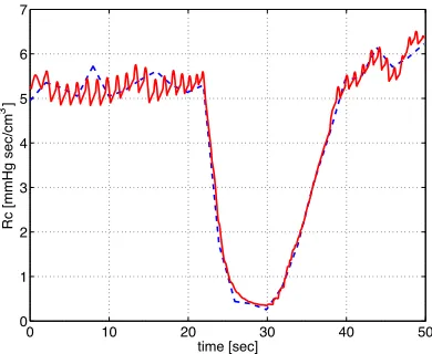
together with the other parameters. Following the parameter estimation we used the predicted time-varying response to propose a cerebral regulation model. The most promising model analyzed had the form

R = Rmet+Rmyo+Rneu, (17)

dRmet

dt =

−Rmet+ ˜Rmet(qc)

τmet

,

dRmyo

dt =

−Rmyo+ ˜Rmyo(pac)

τmyo

,

dRneu

dt =

−Rneu+kneuCach(pa)

τneu

,

where Rmet [ml/sec mmHg] is the contribution from the metabolic regulation,

Rmyo [ml/sec mmHg] is the contribution from myogenic regulation, and Rneu

[ml/sec mmHg] is the contribution from neurally mediated control. Note,Rmetis

modeled as a function of cerebral flowqc [ml/sec], while myogenic contribution

0 10 20 30 40 50 0

1 2 3 4 5 6 7

time [sec]

Rc [mmHg sec/cm

3]

Figure 6: Cerebrovascular resistance predicted using a piecewise linear function (16) (blue) versus the control function (red) proposed in (17).

neurogenic contribution is modeled as a function of arterial pressurepa[mmHg].

It is believed that a potential neurogenic contribution to cerebral vasoregulation is both cholinergic and adrenergic in nature. Therefore we let the set-point equation use concentration of acetylcholine Cach (dimensionless). The concentration of

acetylcholine was computed similar to the open loop heart rate model, see equa-tion (2). For the metabolic and myogenic contribuequa-tions the control funcequa-tions R˜

were sigmoidal functions similar to the one given in (15). Results of the two con-trol models (17) and (16) are shown in Fig. 4. It should be noted that if we omitted any part of the proposed control function we were not able to reproduce the dy-namic found from the piecewise linear function. One thing should be kept in mind is that both the spline model (16) and the differential equations model (17) has 26 parameters. Ideally, it would be better if the cerebral regulation model contained fewer parameters.

2.4

Parameter estimation and model validation

typical measurements include arterial pressure and cerebral flow velocity.

To solve the inverse problem, one can invoke optimization techniques to es-timate a set of model parameters that minimize the least squares error between computed and measured quantities. Whether the parameters for the mathematical model can be estimated assuming sufficient and error-free data is subject to an a priori identifiability analysis. Two aspects typically have to be investigated: First using sensitivity analysis we are able to split model parameters in two sets include: ”sensitive” and ”insensitive” parameters. Sensitive parameters are characterized as parameters where variation in the parameter values invoke a significant change in the model output (see Fig. 7), while a change of insensitive parameters has a negligible impact on the model output. Second, among sensitive parameters, correlations can be present. This type of model dependencies can be predicted accurately for linear models, but for nonlinear models it is more difficult to ana-lyze the system. Once a set of identifiable parameters have been identified, these parameters can be estimated using nonlinear optimization techniques. Following the approach put forward in [6, 31, 5] we describe each of the three components in detail.

Sensitivity analysis

Sensitivities are computed with respect to output vectory(heart rate for the open loop model summarized in (3) and blood pressure and blood flow velocity for the closed loop model summarized in (13)). For both of these models, the nominal parameter values range several orders of magnitude, e.g. for the small closed loop model analyzed in [31] the parameter Em ≈ 0.05, whileCvs ≈ 36. To compute

sensitivities more accurately, we scaled the parameters by the natural logarithm, i.e., the model input to the optimizer is given byθ˜= ln(θ).

Using the scaled parameters sensitivities can be computed as the change in the output variables with respect to the parameters, the absolute sensitivity is defined by

Si,k(t,θ˜) =

∂yk(t, θ)

∂θ˜i

θ0

, (18)

where θ0, denotes the nominal values for the parameters. Even though parame-ters are scaled, quantities compared may still have different units (e.g. pressure and velocity in the closed loop model), thus it is appropriate to analyze relative sensitivities defined as

Sik(t,θ˜) =

∂yk(t, θ)

∂θ˜i

˜

θi

yk(t, θ)

θ0

Note, for the open loop model Si,k is computed with respect to one output, heart

rate, while for the closed loop model both pressure and velocity are concatenated together to provide one long output vector of length2N, thus the length ofSi,kis

2N. As discussed in [6, 4] the sensitivities can either be found using automatic differentiation, by setting up a set of analytical equations, or using finite differ-ences. The finite difference approximation of the sensitivities is less accurate, but for most practical applications including those studied here, finite difference approximations provides sufficient accuracy. This should seen in the light of the high likelihood of introducing errors in analytical sensitivity calculations, in par-ticular for models that has many parameters, e.g., if a model has two outputs and 21 parameters the system 2_×21 = 42 sensitivity equations should be derived. An alternative approach is to use automatic differentiation to derive sensitivity equations, but these methods are computationally ineffective in particular if the differential equations are solved using Matlab. More efficient packages exist in C and Fortran, but these have not been analyzed for this study.

Using finite differences, the derivatives in the sensitivity equations can be computed using the forward difference approximation

∂yk

∂θ˜i

≈ yk(t,θ˜+he_hi)−yk(t,θ˜),

where

ei =

"

0. . .0

i

b1 0. . .0

#T

is the unit vector in thei’th component direction.

To rank the parameters from the most to the least sensitive, we used a scaled 2-norm to get the total sensitivity,Si, to thei’th parameter

Si =

1 2N

2N

X

j=1

S_i,k2

!1/2

.

Figs. 7 and 8 show examples of the sensitivity analysis. Fig. 7 shows ranking and time varying sensitivities for the open loop model using data from a healthy young subject. Note the change in solution arising from varying the insensitive parame-terτI barely changes the model solution, while a significant change in heart rate

is observed when the sensitive parameter ζP is varied. Fig. 8 shows the average

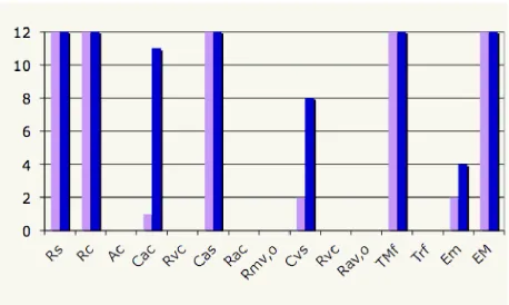
the closed loop model. The specific closed loop model used for these calcula-tions included 4 vascular and one ventricular compartments, the model had 21 parameters.

It should be noted that the classical sensitivity analysis described above is a local analysis, and thus sensitivities depend on the values of the parameters. In this study the goal is to use sensitivity analysis to rank parameters in order of sensitivity and use this ranking in conjunction with results from subset selection to identify a set of parameters that can be estimated for all subjects. This is done prior to actual parameter estimations, thus the sensitivity ranking was computed using nominal parameter values.

In summary, results from the sensitivity analysis showed that both models in-clude both sensitive and insensitive parameters. Sensitive parameters can often be estimated using optimization techniques, while insensitive parameters are difficult to estimate since a small change in the parameter value gives rise to a small change in the solution. This can become problematic when models are used to extract bi-ological information from estimated parameter values as done in the studies sum-marized here. However, it should be noted that identifiability is a mathematical notion. For biological implications the precise values of parameters are not always important as long as they have certain characteristics, e.g., like being positive. An alternative method is to use generalized sensitivity analysis, which provide more insight into the dynamics of the model.

Subset selection

Subset selection can be approached using a number of methods as described in [32]. Below we outline the method used in [31]. In this study subset selec-tion analyzes the Jacobian matrix (r′

=dr/dθ) computed from the residual vector

r (see equations (3) and (13)). The entry at row iand column j of the Jacobian is ∂ri/∂θj. The Jacobian, singular value decompositionr′ = UΣVT is used to

obtain a numerical rank for r′

. This numerical rank is then used to determine ρ

parameters that can be identified given the model outputydefined in (3) and (13). QR decomposition is used to determine theρidentifiable parameters to which our system is sensitive as a group. This differs from sensitivity analysis, which finds parameters to which our system is individually sensitive. To estimate the number of uncorrelated parameters we used an error estimate in our computation of the Ja-cobian as a lower bound on acceptable singular values. For example, in the studies analyzed here we used Matlabs differential equations solver ODE15S with an ab-solute error tolerance of10−₆

, i.e., the error of the numerical model solution is of order10−₆

and the error in the Jacobian matrix is approximately√10−₆

= 10−₃

0.0 0.1 0.2 0.3 0.4 0.5 0.6 0.7 0.8

0 10 20 30 40 50

0 0.1 0.2 0.3 0.4 0.5 0.6 time [sec] sensitivity ζ P k S τ I

0 10 20 30 40 50

0.95 1 1.05 1.1 1.15 1.2 1.25 1.3 1.35 time [sec] HR [beats/s] HR New HR

0 10 20 30 40 50

0.95 1 1.05 1.1 1.15 1.2 1.25 1.3 1.35 time [sec] HR [beats/s] HR New HR

0 10 20 30 40 50

0.95 1 1.05 1.1 1.15 1.2 1.25 1.3 1.35 time [sec] HR [beats/s] HR New HR

0.0 0.2 0.4 0.6 0.8 1.0 1.2 1.4 1.6 1.8 2.0

Rc Ac _{Em Rm}v,o _Cvs _TMf Rs _EM Trf _Cas _Rvc _Cac _Rac

Rav,o Cvc

Figure 8: Sensitivity ranking for a 5 compartment (systemic arteries and veins, cerebral arteries and veins, and the left ventricle) closed loop model. Sensitivities are computed with respect to arterial pressure and cerebral blood flow velocity. A weighted 2-norm was used to obtain an average sensitivity over the entire time series.

Consequently, singular values should not be smaller than 10−3

. Since the error of the Jacobian is an approximation, the smallest singular value that we accept is 10−₂

. Once the number of identifiable parameters has been determined, we find the most dominant parameters by performing a QR decomposition with col-umn pivoting on the most dominant right singular vectors. The process begins by choosing the most sensitive parameter in a way similar but not identical to the sensitivity analysis of the previous section, the column with largest 2-norm is chosen. The algorithm chooses additional parameters in a way that keeps the con-dition number of the chosen columns small. Below we summarize subset selection method as an algorithm.

Subset selection algorithm:

1. Given an initial parameter estimate, θ0, compute the Jacobian, r′(θ0) and the singular value decomposition r′

= UΣVT_{, whereΣis a diagonal}

ma-trix containing the singular values of r′

in decreasing order, and V is an orthogonal matrix of right singular vectors.

2. Determineρ, the numerical rank of r′

smallest allowable singular value.

3. Partition the matrix of eigenvectors in the formV = [VρVn−_ρ].

4. Determine a permutation matrix P by constructing a QR decomposition with column pivoting, forVT

ρ . That is, determineP such that

V_ρTP =QR,

whereQis an orthogonal matrix and the firstρcolumns ofRform an upper triangular matrix with diagonal elements in decreasing order.

5. UseP to reorder the parameter vectorθ0 according toθˆ0 =PTθ0.

6. Make the partitionθˆ0 = [ˆθ0,ρθˆ˜0,n−_ρ]whereθˆ_0,ρcontains the firstρelements

ofθˆ0. Fixθˆn−ρat the a priori estimateθˆ0,n−ρ.

7. Compute the new estimate of the parameter vectorθˆby solving the reduced-order minimization problem

ˆ

θ=arg min_θJ(θ), withθˆn−_ρfixed at nominal valuesθˆ_0,n−_ρ.

Fig 9 shows possible subsets of identifiable parameters from the same model that we used to show results of the sensitivity analysis. The model used for this study included 4 vascular and one ventricular compartments, the model had 21 parameters, and out of these only 4 could be estimated reliably given arterial blood pressure and cerebral blood flow velocity data measured during sitting. It should be noted that this model did not include any control mechanisms.

Optimization techniques

Figure 9: Subsets computed for 16 healthy young and 16 healthy elderly subjects using a 5 compartment closed loop model combined with arterial blood pressure and cerebral blood flow velocity data.

have several stationary points that do not correspond to the lowest value of the fitness landscape. Local search methods, like the Levenberg-Marquardt method, easily gets trapped in one of the local minima rather than finding the global mini-mum. To explore the whole search space one needs global search methods and if possible a physiological range for realistic values. Unfortunately, these methods converge very slowly once near a minimum. In contrast, gradient-based meth-ods are efficient optimizers for nonlinear LQP’s once a sufficiently good initial guess for the parameter values is available. Thus a recommendable strategy is to use the solutions from the global search as initial guesses for local optimiza-tion. In this way, one reduces the chance of missing the global minimum and the determination of all the minima is precise and fast. In the problems analyzed and discussed here we used the Nelder-Nead method (a gradient free global opti-mization method) to estimate parameters for the open loop model and a gradient based method (a Levenberg-Marquart method with Trustregions) for the closed loop model. Both methods worked well, but the Nelder-Mead method was signif-icantly slower, while the Levenberg-Marquart method required that we estimated initial parameter estimates carefully.

3

Discussion

Below we summarize and discuss result reported in [24, 25, 30, 18, 19, 20, 21, 22, 6, 31, 5]. We divide the presentation into three subsections; open loop model, closed loop model, and syncope.

3.1

Open Loop model

Results with the open loop model have been reported in [24, 25, 21, 22, 7] re-sults were obtained with the STS and HUT protocol. In [21] we analyzed STS data from three groups of subjects including healthy young, healthy elderly, and hypertensive elderly healthy young subjects, and in [22] we analyzed both STS and HUT data from five young subjects. For both studies all model parameters were predicted using the Nelder-Mead optimization method. Results showed that standard deviations were typically high, however, for both studies we were able to detect interesting differences between the groups of subjects. In [21] (results

50 60 70 80 90 100 110 120 130 140 40

50 60 70 80 90 100 110 120

p [mmHg]

n [1/sec]

50 60 70 80 90 100 110 120 130 140 40

50 60 70 80 90 100 110 120

p [mmHg]

n [1/sec]

50 60 70 80 90 100 110 120 130 140 40

50 60 70 80 90 100 110 120

p [mmHg]

n [1/sec]

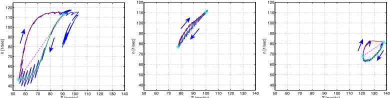
Figure 10: Example hysteresis depicting changes in baroreflex firing rate (n) as a function of mean blood pressure (p). Results are shown for a healthy young subject (left), a healthy elderly subject (center), and a hypertensive elderly subject (right). Dashed lines through the curves were used to determine the overall slope, and arrows indicate responses to change in pressure. Baroreceptor hysteresis is an important feature that demonstrates how baroreflex controls adapt in response to to differences in vascular compliance that occur with aging.

for most subjects the hysteresis loop was not closed, indicating that within the timeframe included in the experiments the pressure does not return to the value obtained during sitting. This may indicate that part of the regulation is not work-ing as expected. In addition, comparison of parameters between groups revealed that parameterskI, kL, β, τd, τach, andMP changed significantly between groups.

These results were obtained using ANOVA analysis using 20 data sets for each group. Data from 10 subjects (2 experiments per subject) were analyzed. It should be noted that these results were obtained without any applying any model and pa-rameter reduction techniques. Seen from a physiological point of view observing differences in the given parameters are reasonable, reduction inkIandkLindicate

that with age and hypertension, the firing rate sensitivity to changes in pressure is reduced, increase of β andτd, indicate that with age and hypertension, the delay

in onset of sympathetic response is increased and that parasympathetic dampen-ing of the sympathetic response is attenuated, finally τach increase with age, but

decrease with hypertension. An age related increase in τach suggests that with

age it takes longer for the parasympathetic response to reach its maximum effect, while the decrease with hypertension, may be compensating for the fact that the vessels are significantly stiffer. Finally MP is increased with both age and

hy-pertension indicating that parasympathetic regulation plays a more important role than subsequent sympathetic stimulation of heart rate.

Results from [22] (see Fig. 11 ) showed that there were significant differences between results from the STS and HUT procedures. Comparing the two tests showed a much larger increase in heart rate during HUT than during STS and a more significant drop in blood pressure during STS than during HUT, leading to more pronounced changes in firing rate and sympathetic/parasympathetic tone. Another noticeable difference is the change in the area of the hysteresis loop: the loop is significantly wider during STS than during HUT. Finally, we noticed that during HUT heart rate decrease during the initial preparation to tilt (before any blood pressure drop was observed), while during STS heart rate increased before the subject changed posture (the latter observation was also found in our first study [21]. This initial drop in heart rate is associated with a slight increase in blood pressure (compare panels A and E). This may be due to a short increase in venous return due to hydrostatic pressure difference imposed between the heart and the head. On the other hand the increase in heart rate immediately before standing may, as explained earlier, be due to vestibular and muscle sympathetic activation.

Re-0 10 20 30 40 50 50

100 150

time [sec]

pa [mmHg]

0 10 20 30 40 50

50 100 150

time [sec]

pa [mmHg]

70 80 90 100 110

20 40 60 80 100

p [mmHg]

n [Hz]

70 80 90 100 110

20 40 60 80 100

p [mmHg]

n [Hz]

0 10 20 30 40 50

1.2 1.3 1.4 1.5 1.6 1.7

time [sec]

HR [beats/s]

0 10 20 30 40 50

1.2 1.3 1.4 1.5 1.6 1.7

time [sec]

HR [beats/s]

sults of this analysis showed that some parameters are very insensitive including

τI, kI, ζS, and τach. Results varying a sensitive parameter, an intermediate

pa-rameter and an insensitive papa-rameter are showed together with the ranking. One aspect not done for this study is to analyze if any of the sensitive parameters are correlated, more analysis is needed to investigate potential correlations. Such cor-relations are likely to exist, some initial attempts to study those have been done by Fowler [7] comparing results obtained with Nelder-Mead with both implicit filtering and using a genetic algorithm to optimize model parameters.

3.2

Closed Loop model

440 460 480 500 520 65

70 75 80 85 90 95 100 105 110 115

time [sec]

pa [mmHg]

440 460 480 500 520

35 40 45 50 55 60

time [sec]

vc [cm/sec]

Figure 12: Model generated arterial pressure (top panel) and cerebral blood ve-locity (lower panel) when respiratory effects are included. The resulting curves are realistic and in accordance with measurements

model was significantly simpler, and because we used subset selection, we were able to predict dynamics for two groups of subjects including 16 healthy young subjects and 16 healthy elderly subjects. Results of this comparison showed that both cerebral resistance and compliance were modulated by aging. Results also showed that the total resistance was increased and that TM, f time for systolic

pressure was increased.

All closed loop models were able to predict both blood pressure and cere-bral blood flow velocity as shown in Fig. 13, however, only models were sub-set selection and sensitivity analysis were used could be analyzed against several datasets. The more advanced models (including more compartments) simply had to many parameters, thus making it very tedious to achieve good predictions of the data. In future work, we plan to apply subset selection to the more complex models, and with this method we anticipate that even the more complex models can be validated against multiple datasets, allowing identification and prediction of biomarkers.

The results shown in Fig. 13 were obtained with the complex control model developed in [19, 20]. In this figure we show how the closed loop compartmental model allows prediction of arterial blood pressure (pa) and cerebral blood flow

ve-locity (vc) during postural change from sitting to standing. The figures shows the

40 50 60 70 80 90 0

50 100 150 200

pa [mmHg]

40 50 60 70 80 90

−50 0 50 100 150

time [sec]

vc [cm/s]

45 46 47 48 49 50

50 100 150

pa [mmHg]

45 46 47 48 49 50

0 50 100

time [sec]

vc [cm/s]

65 66 67 68 69 70

50 100 150

pa [mmHg]

65 66 67 68 69 70

0 50 100

time [sec]

vc [cm/s]

80 81 82 83 84 85

50 100 150

pa [mmHg]

80 81 82 83 84 85

0 50 100

time [sec]

vc [cm/s]

Figure 13: Pressure [mmHg] (top panel) and flow velocity [cm/sec] (bottom pan-nel) for STS with respiratory mechanical effect included.

and during standing (for t _∈ [80 : 85] sec). Note, while the model was able to predict the amplitude and approximate shape of the waveform, this type of model cannot predict the wave reflections observed in the data. To predict these, it is necessary to use a fluid dynamics model, that more realistically allows modeling of the wave propagation.

of CO2and O2, this model is described in [5, 4]. The second figure (Fig. 14) shows not only effect on arterial pressure but on the internal states as well. It should be noted that respiration also affects the overall flow distribution and favors some braches at the expense of others and moreover Starlings law of the heart follows as a result. Furthermore, including mechanical coupling with respiration also af-fect model parameter values. Especially, parameters related to the ventricles and the control mechanisms are sensitive to effect of respiration. Surprisingly the im-pact of mechanical movement giving rise to respiration is somehow strong as see in Fig. 14, where the movement of the diaphragm during respiration is seen to be significant.

3.3

Syncope

Control mechanisms of the cardiovascular system play an important role in adap-tation to postural changes during everyday activities. Syncope (meaning a pause in music) is the medical term for temporary loss of consciousness or fainting. Syncope is a common and significant medical problem that accounts for 3-6% of emergency rooms visits and hospital admissions every year and in some cases may hallmark a significant underlying morbidity. Syncope is multifactorial and can be triggered from many different inputs into the central and peripheral auto-nomic systems. It often manifest as an abrupt loss of muscle tone with/without falling accompanied by a decline in blood pressure, blood flow to the brain, and heart rate, the latter may even lead to temporary cardiac arrest. This presentation may have clinical prodromes and changes in autonomic nervous system firing for minutes before the actual loss of consciousness occurs. Syncope is considered to be a reflex mechanism, protecting the vital organs (mainly the brain) from lack of perfusion.

-35 -30 -25 -20 -15 -10 -5 0 60

70 80 90 100 110 120 130

Mean pressure in upper torso

F

lo

w

[

m

l]

Flow effects of amplitude and depth on CO

Amplitude Depth

Bradycardia or slow heart rate typically occurs later when blood pressure falls be-low certain threshold. In the model of HUT syncope appear approximately after 30 minutes as a sudden incident as a result of a crash in the control system where the effect of the controls saturates.

In the example discussed here the reduction in flow is initiated by the sudden drop in blood pressure observed during HUT, followed by compromised auto-nomic and cerebral autoregulation. In contrast to the heart rate regulation a uni-fying description of pressure changes shows that multiple simultaneous control mechanisms may be important in order to understand the experiments.

There are many reasons to use the model to analyze questions related to syn-cope, most importantly, it is not well know what mechanisms triggers syncope. A number of theories put forward to explain the phenomena [15]. How each of these theories impact pressure, flow, and HR dynamics could be studied using the proposed models.

To model dynamics during syncope we used the model illustrated in Fig. 5 modified to include intermediate control mechanisms essential for describing dy-namics of HUT experiments over longer time scales (>35 min). To do so it is important to account for dynamics of the venous pump, functioning to prevent pooling of flow in the extremities due to effects of gravity. This type of dynamics was not included in the original closed loop model, which was developed to study dynamics over a short time scale (<2 min). To model this we included a fluid shift compartment at the level of the legs. Through this compartment fluid was continu-ously transfered from the cardiovascular system to the extravascular environment. Consequently, during regulation, a combination of control mechanisms including arterial resistance and venous compliance regulation, fluid shift and dead volumes are regulated in this study. In addition, we incorporated a slight tension of the diaphragm The resulting model nicely describes the HUT experiments as shown in Fig. 15. In particular notice, how well the model reproduce data. The crash happens in the model when the arterial compliance regulation reach its saturation. Thus the heart rate cannot manage to regulate the system alone, venous return declines and the system breaks down resulting in syncope.

4

Conclusion

60

60 70 160

140

120

100

80

120

80 90 100 110

500 1000 1500 2000 2500 3000

40

40

20 60 80 100 120 140 160 180 200

pa [mmHg]

pa [mmHg]

HR [bpm]

time [sec]

were discussed open-loop models that use blood pressure as an input to predict heart rate, and a closed loop model that allow prediction of both blood pressure and blood flow velocity. We showed how these models could be used to predict patient specific data by solving the inverse problem estimating a set of model parameters that allow prediction of patient specific dynamics. Two analysis tec-niques were investigated, and prove to be essential to obtain good results: sen-sitivity analysis, which allow us to rank model parameters from the most to the least sensitive, and subset selection, which allow us to identify correlation among model parameters. The sensitivity ranking can be used to identify insensitive pa-rameters that cannot be estimated given data, and allowed us to identify essential components of the model. Subset selection allowed us to predict a subset of un-correlated parameters among the sensitive parameters, which can be reliably be estimated using the available data. Finally, we show how these models can be used to model clinical events (syncope), and using this example, we have shown that this type of modeling approach has potential to be used for better understand-ing of underlyunderstand-ing mechanisms triggerunderstand-ing syncope. Another important outcome is that the type of models developed here allow prediction of internal states, which cannot be measured experimentally.

However, the models themselves have a number of limitations. First, the spar-sity of data used for prediction of dynamics in the closed loop models discussed above, is probably the main limitation is obtaining good patient specific models. As discussed earlier, only 4-6 parameters can be estimated reliably given these data. Another limitation, not of the models, but of the patient specific analysis is that without measurements of cardiac output it is difficult to get flow distributions correct. Many different estimates of cardiac output can be distributed to obtain the correct arterial pressure and cerebral blood flow velocity, and as discussed in [31], the models analyzed here typically underestimates cardiac output. Consequently, one important suggestion we can put forward for researchers interested in using the proposed modeling tools discussed here is to incorporate some measurements of cardiac output.

Another important lesson we learned (discussed in [6]), is that for any given application, it is essential to include as few compartments as necessary to model the proposed dynamics, and then be conservative in reducing the number of pa-rameters estimated to predict patient specific dynamics.

5

Acknowledgements

The authors wish to thank graduate students involved with this project includ-ing Laura Ellwein, Dept of Biomedical Engineerinclud-ing, Marquette University, Scott Pope, SAS Corp, Raleigh, NC, April Alston, Dept of Math, NCSU, and numer-ous undergraduate students participating in research and REU program at NCSU. Furhtermore, authors would like to thank Hien Tran and Tim Kelley, Department of mathematics, NCSU. The work by M.S. Olufsen was supported in part by NSF-DMS grant # 0616597 and NSF-OISE grant# 0437037. V. Novak, director of the SAFE Laboratory at BIMDC was supported by NIH-NIA Harvard Older Ameri-can Independence Center 2P60 AG08812-11A1, Core B.

References

[1] Allen L.J.S. An Introduction to Mathematical Biology. Pearson Education, Up Sadddle River, NJ, 2003.

[2] Danielsen M. Modeling of feedback mechanisms which control the heart func-tion in a view to an implementafunc-tion in cardiovascular models. PhD Thesis, Roskilde University, Denmark. Text No 358, 1998.

[3] DeVault K., Gremaud P., Zhao P., Vernieres G., Novak V., and Olufsen M.S. Blood flow in the circle of Willis: Modeling and calibration. SIAM J Multiscale Anal Simul, 7:888–909, 2008.

[4] Ellwein L.M. Cardiovascular and Respiratory Regulation, Modeling and Pa-rameter Estimation.. PhD Thesis, Applied Mathematics, NC State University, Raleigh, NC. 2009.

[5] Ellwein L.M., Pope S.R., Xie A., Batzel J.J., Kelley C.T., and Olufsen M.S. Modeling cardiovascular and respiratory dynamics in congestive heart failure. Submitted, 2009.

[6] Ellwein L.M., Tran H.T., Zapata C., Novak V., and Olufsen M.S. Sensitivity analysis and model assessment: Mathematical models for arterial blood flow and blood pressure. J Cardiovasc Eng, 8:94–108, 2008.

[8] Guyton A.C. and Hall J.E. Textbook of medical physiology. WB Saunders, Philadelphia, PE, 9th ed, 1996.

[9] Johnson P., Shore A., Potter J.F., Panerai R.B., and James M. Baroreflex sen-sitivity measured by spectral and sequence analysis in cerebrovascular disease - methodological considerations Clin Auton Res, 16: 270–275, 2006.

[10] Jose A. and Collison D. The normal range and determinants of the intrinsic heart rate in man. Cardiovasc Res, 4: 160–167, 1970.

[11] Kaufmann H., Biaggioni I., Voustianiouk A., Diedrich A., Costa F., Clarke R., Gizzi M., Raphan T., and Cohen B. Vestibular control of sympa-thetic activity: An otolith-sympasympa-thetic relfex in humans. Exp Brain Res, 143: 463–469, 2002.

[12] Kyrylov V., Severyanova L.A., and Vieira A. Modeling Robust Oscillatory Behaviour of the Hypothalamic-Pituitary-Adrenal Axis. IEEE Trans Biomed Eng, 52:1977–1983, 2005.

[13] Liang K.H., Krus D.J., and Webb J.M. K-fold crossvalidation in canonical analysis. Multivariate Behavioral Resarch, 30:539–546, 1995.

[14] Low P.A. and Bannister R.G. Multiple System Atrophy and Pure Autonomic Failure. In: Low P.A.(eds). Clinical Autonomic Disorders. Lippincott-Raven Publishers, Philadelphia, PE, pp. 555–575, 1997.

[15] Mosqueda-Garcia R., Furlan R., Tank J., and Fernandez-Violante R. The elu-sive pathophysiology of neurally mediated syncope. Circulation, 102: 2898– 2906, 2000.

[16] Olufsen M.S. Structured tree outflow condition for blood flow in larger sys-temic arteries. Am J Physiol, 276:H257–H268, 1999.

[17] Olufsen M.S., Nadim A., and Lipsitz L.A. Dynamics of cerebral blood flow regulation explained using a lumped parameter model. Am J Physiol, 282:R611–R622, 2002.

[19] Olufsen M.S., Tran H.T., and Ottesen J.T. Modeling cerebral blood flow con-trol during posture change from sitting to standing. Cardiovasc Eng, 4(1):47– 58, 2004.

[20] Olufsen M.S., Ottesen J.T., Tran H.T., Ellwein L.M., Lipsitz L.A., and No-vak V. Blood pressure and blood flow variation during postural change from sit-ting to standing: model development and validation. J Appl Physiol, 99:1523– 1537, 2005.

[21] Olufsen M.S., Tran H.T., Ottesen J.T., Lipsitz L.A., and Novak V. Model-ing baroreflex regulation of heart rate durModel-ing orthostatic stress. Am J Physiol, 291:R1355–R1368, 2006.

[22] Olufsen M.S., Alston A.V., Tran H.T., Ottesen J.T., and Novak V. Modeling heart rate regulation, Part I: Sit-to-stand versus head-up tilt. J Cardiovasc Eng, 8:73–87, 2008.

[23] Opthof T. The normal range and determinants of the intrinsic heart rate in man. Cardiovasc Res, 45:173–176, 2000.

[24] Ottesen J.T. Modeling of the baroreflex-feedback mechanism with time-delay. J Math Biol, 36:41–63, 1997.

[25] Ottesen J.T. Nonlinearity of baroreceptor nerves. Surv Math Ind, 7:187–201, 1997.

[26] Ottesen J.T. General Compartmental Models of the Cardiovascular System in Mathematical Modelling in Medicine. IOS press, Amsterdam, pp. 121–138, 2000.

[27] Ottesen J.T. Modeling the dynamical baroreflex-feedback control. Math Comp Mod, 31:167–173, 2000.

[28] Ottesen J.T. and Danielsen M. Modeling ventricular contraction with heart rate changes. J Theor Biol, 222:337–346, 2003.

[29] Ottesen J.T. Valveless pumping in a fluid-filled closed elastic tube-system: one-dimensional theory with experimental validation. J Math Bioll, 46:309– 332, 2003.