FETTER, WILLIAM WOODROW. Effects of Far-Side and Side-Street Bus Stops on the Saturation Flow Rate of Signalized Intersections. (Under the Direction of Dr. Joseph E. Hummer.)
As the use of public transit buses increases, it is important to understand how bus
stops affect the surrounding traffic stream, especially with regards to intersection
saturation flow rate. The HCM 2000 and other sources have addressed the effect of
near-side bus stops, but no one has successfully analyzed bus stops on the far-near-side or near-
side-streets of an intersection. The purpose of this study was to determine the effects that both
far-side and side-street bus stops have on the saturation flow rate at a signalized
intersection.
To determine these effects, a set of analytical equations was derived for each bus
stop type. The methodology for these equations required calculating the number vehicles
processed through the intersection during each of three defined time periods within the
green indication of a cycle. The time periods were divided according to how the buses
blocked the traffic: full blockage (period 1), partial blockage (period 2), and no blockage
(period 3). The average number of vehicles processed during a cycle was determined by
multiplying each of the vehicles processed in a time period by the probability of buses
stopping in that time period and then summing them together. The average number of
vehicles processed was then divided by the ideal number of vehicles processed (obtained
from simulation) to obtain an adjustment factor. Applying this factor to the saturation
flow rate calculated the effects due to the bus stop.
To analyze the ability of the equations to predict saturation flow rates, they were
tested using a variety of variable inputs and compared with CORSIM simulation runs
using the same inputs. Sensitivity tests were also performed to determine how the
equations reacted under a variety of variable extremes. The results from these analyses
were not exactly ideal and, as a result, the equations could only be partially validated.
Overall, while it appears that the method for determining saturation flow rate
according to the HCM is inaccurate, an adequate replacement method has not yet been
Effects of Far-Side and Side-Street Bus Stops
on the Saturation Flow Rate of Signalized Intersections
by
William W. Fetter
A thesis submitted to the Graduate Faculty of
North Carolina State University
in partial fulfillment of the requirements for
the Degree of Master of Science
Department of Civil Engineering
Raleigh, NC
2007
APPROVED BY:
_________________________ _________________________
Nagui M. Rouphail
John R. Stone
_________________________
Chair of Advisory Committee
BIOGRAPHY
The author was born and raised on a farm near Charlotte, North Carolina. On the
farm, he learned the value of hard work and determination and gained valuable life
lessons from his father. At an early age, it was instilled that having a strong educational
background was very important to being successful. Two of his father’s favorite quotes
were “no one can ever take away your education” and “without an education, you’ll
never become successful”. Heeding his advice the author enrolled in several vocational
classes while attending high school, at one point causing him to be enrolled in three
different schools at the same time. The author graduated from Sun Valley High School in
June 2000.
After graduating high school, the author attended the William States Lee College
of Engineering at the University of North Carolina at Charlotte. It was here that the
author discovered transportation engineering and focused most of his studies around it.
While attending classes the author met his future wife, Maya, and the two were soon
engaged. In his last attending years, the author received a large push from several
members of the faculty to attend graduate school at NC State University, specifically
under the direction of Dr. Joseph Hummer. Eventually the author applied and soon was
accepted to NC State. The author graduated with a Bachelor Degree in Civil Engineering
in December 2004.
The author then moved to Raleigh and started attending classes at NC State.
During the summer of 2005, the author married and his wife joined him in Raleigh.
While attending the graduate school the author would work during the day at local
engineering firms and attended graduate school classes in the evening. At graduate school
the author focused his studies on transportation and traffic engineering. The author
ACKNOWLEDGEMENTS
I would like to extend my appreciation to my advisor Dr. Joseph Hummer who
has provided me with priceless advice and challenged me to see transportation
engineering from different perspectives. I would also like to thank Dr. John Stone and Dr
Nagui Rouphail for the instruction I received in their classes and their participation in my
thesis committee.
I also would like to acknowledge Dr. Rajaram Janardhanam at UNC Charlotte
who pushed me to attend graduate school. He advised me where to go and under whom to
study. Without his encouragement during my undergraduate career, I do not think I
would ever have chosen this path.
I also extend my appreciation to my loving wife Maya Fetter who has stood
beside me while I attempted to divide by time between being a student, a husband, and a
family provider all at once. Without her support, I would never have had the strength to
complete graduate school.
My thanks are also extended to my mother Pamela, my sister Kathryn, and the
rest of my family who have always supported me in my goals. I also extend thanks to my
father, Edward, who provided me with unforgettable life lessons and advice that I will
never forget. It is through these lessons and advice that he has continued to support and
TABLE OF CONTENTS
LIST OF FIGURES... vi
LIST OF TABLES ... vii
CHAPTER 1 - INTRODUCTION ... 1
Background ... 1
Scope... 2
Project Objectives ... 3
Thesis Outline... 4
CHAPTER 2 - LITERATURE REVIEW... 5
Current Literature... 5
Related Research Topics... 8
Previous Research ... 14
Literature Review Conclusions... 16
CHAPTER 3 - METHODOLOGY ... 18
Model Formulation ... 18
Far-Side Bus Stop ... 19
Side-Street Bus Stops ... 29
Saturation Flow Rate Adjustment Factor ... 30
Experiment Design... 37
Model Analysis ... 39
CHAPTER 4 - ANALYSIS RESULTS... 43
Initial Model Analysis ... 43
Equation Calibration ... 47
Equation Validation... 53
Calibrated Model Analysis ... 54
Sensitivity Analysis... 58
Application to Transit Managers ... 65
CHAPTER 6 - RECOMMENDATIONS ... 69
Future Work ... 69
REFERENCES... 72
APPENDICIES ... 74
Appendix A: Far-Side Simulated and Equation Calculated Data ... 75
Appendix B: Side-Street Simulated and Equation Calculated Data ... 108
Appendix C: Far-Side Simulated and Calibrated Equation Calculated Data ... 125
Appendix D: Side-Street Simulated and Calibrated Equation Calculated Data ... 138
Appendix E: Far-Side Sensitivity Analysis ... 147
Appendix F: Side-Street Sensitivity Analysis Data... 166
LIST OF FIGURES
Figure 1. Diagram of Near-Side and Far-Side Bus Stops ... 15
Figure 2. Diagram of Far-Side and Side Street Bus Stops... 19
Figure 3. Diagram of Time and Space Relationship of BT ... 21
Figure 4. Diagram of Stop Bar Location and Vehicle Storage Spaces For Far-Side Bus Stop ... 22
Figure 5. Linear Relationship Between BST and the Number of Vehicles Processed ... 26
Figure 6. Diagram of Time Periods and Relationships... 27
Figure 7. Diagram of CORSIM Network Used in Analysis ... 34
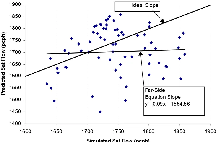
Figure 8. Equation Predicted Saturation Flow Rate Values for Far-Side Bus Stops ... 46
Figure 9. HCM Predicted Saturation Flow Rate Values for Far-Side Bus Stops ... 47
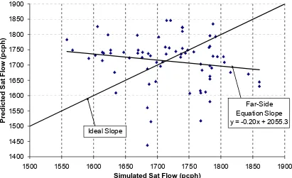
Figure 10. Calibrated Equation Predicted Saturation Flow Rate Values for Far-Side Bus Stops... 56
Figure 11. Calibrated HCM Predicted Saturation Flow Rate Values for Far-Side Bus Stops... 57
Figure 12. Storage Length in Vehicles versus Storage Length in Feet... 58
Figure 13. Sensitivity Plot for Calibrated Far-Side Equations ... 61
Figure 14. Sensitivity Plot for Calibrated Side Street Equations... 63
LIST OF TABLES
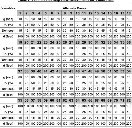
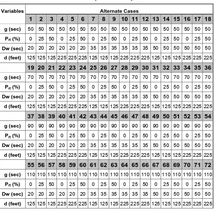
Table 1: Far-Side Bus Stop Case Descriptions for Calibration ... 39
Table 2: T-Test and F-Test Results for Initial Analysis ... 44
Table 3: Initial Difference in Simulated and Predicted Values ... 45
Table 4: Simulated Probabilities of Buses Crossing the Stop Bar During Each Time Period ... 49
Table 5: Predicted Probabilities of Buses Crossing the Stop Bar During Each Time Period ... 49
Table 6. Simulated Probabilities of Buses Stopping in Time Periods When Assumptions are Violated... 52
Table 7: Far-Side Bus Stop Case Descriptions for Validation ... 53
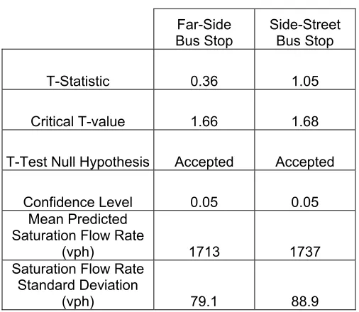
Table 8: T-Test and F-Test Results for Calibrated Analysis ... 54
Table 9: Calibrated Difference in Simulated and Predicted Values ... 55
CHAPTER 1 - INTRODUCTION
Background
The supply of transportation facilities in the U.S. is not keeping up with the
ever-growing demand. From 1960 to 2004, the total number of vehicle-miles driven annually
increased 400% while the total highway centerline miles inventory has only increased by
12% (1).
One solution to managing growing traffic demand is to increase the use of public
transportation. This would decrease the number of vehicles on the roadways and thereby
reduce congestion on the roads and at the intersections. With recent gasoline prices
becoming a burden on the average driver, bus ridership is steadily increasing by about
3% per year in the US, and is seen more often as an attractive approach to transportation
rather than driving one’s own car (1).
Because public transportation is on the rise, it is important to evaluate its impact
on the local traffic stream. Transit buses are primarily found in urban areas and make
frequent stops at designated bus stops that are often located near intersections. At a bus
stop, a bus must first slow down, stop to pick up passengers, and then accelerate back up
into the traffic stream. While all of this is occurring, vehicles behind the bus are delayed
or stopped. Depending on the position of the bus, vehicles may be blocked from
proceeding through or making a turn at the nearby intersection. The impact of buses
making stops can be measured in total traffic delay at the nearby intersection. Since delay
is a function of intersection capacity, capacity must first be calculated in order to
determine transit impact.
The Highway Capacity Manual 2000 (HCM) is the standard reference used to
estimate intersection capacity using a series of adjustment factors based on intersection
properties (2). One of these factors, the bus blockage factor, estimates the effect on
capacity due to buses stopping near an intersection based on the dwell time at a bus stop.
The dwell time is defined as the time from when the bus comes to a complete stop at the
bus stop until the time the bus leaves the bus stop. A close review of the HCM, however,
shows conflicting values of the dwell time in different chapters. This leads to questions
Other sources such as Rodriquez-Seda and Benekohal (3), Wong et. al. (4), and
Holt (5) also have expressed concerns about inaccurate calculations of the effects of
buses on traffic and felt that the blockage factor presented in the HCM (2) was not
satisfactory for all cases and bus stops. By determining what literature had conflicting
information, and what information was not available, areas that needed to be addressed
were determined. By focusing the analysis on those areas the current research gaps were
addressed.
Scope
This project was focused on calculating a saturation flow rate adjustment method
due to the effects of bus stops at nearby signalized intersections. Because intersection
saturation flow rates are a function of capacity and not delay, no delay calculations for
buses and vehicles were performed.
This study was limited to bus stops located on the far-side and on the side-streets
of intersections with respect to the approaching lane segment. The analysis was
performed assuming urban environments, containing intersections with pre-timed
signalized control. Bus routes with short headways were also assumed but the methods
are applicable to any length of bus headway. Actuated signals were not considered in this
study. Only curbside bus stops with no bus bays were analyzed, eliminating the
possibility of traffic maneuvering past a stopped transit bus.
This study was performed on a single lane approach to a “T” intersection where
only through and right-turn movements were permitted. Even though only single lane
roadways were analyzed the methods and concepts produced herein should be applicable
to multilane roads or intersections with four approaches. Application to multilane roads is
possible by applying the evaluation method to the lane containing a bus stop. Since no
other lane or lanes besides the one containing the bus stop will be affected by a bus
stopping, they will not experience the effects due to that stop. Application to multiple
approach intersections is possible by applying the evaluation method to only the approach
in question. If other approaches are present, they are assumed to have negligible effect
green or in the red indication of the study approach and do not depart until past the start
of the next green phase.
Instead of field verification the transit capable modeling software CORSIM was
used to verify the analytical equations presented. This software is widely accepted and
has been proven effective in simulating similar networks as required in this study
according to other researchers such as Jones et. al (6), Wang and Prevedouros (7), and
Luh (8). The simulated intersection in this study was kept completely saturated at all
times in order to measure the effects from the bus stops. A total of 288 far-side and 192
side street CORSIM runs were made with various alternatives to attempt to capture the
effects of a bus stop under a variety of circumstances.
Project Objectives
This research project proposes to estimate the impact of bus stops on the capacity
of a nearby, signalized intersection. It presents a new method of analyzing the effects of
bus stops, based upon bus stop characteristics and locations, and specific defined time
periods within the cycles green time. This new method is based on series of analytical
equations that can be used to predict the saturation flow rate at nearby signalized
intersections due to the effects of bus stops. The presented models were compared to
CORSIM software simulations of a simple saturated roadway network with a single
travel lane, a single bus stop, and a single bus route. The effect on saturation was
performed by simulating operation for an “ideal network” with no bus stops, and
adjusting the calculated “ideal” saturation flow rate according to the analytical equations
to develop “predicted” saturation flow rate values. Simulations were also performed on a
network with bus stops to obtain the “simulated” saturation flow rates values. The
“predicted” and “simulated” saturation values were then compared and subjected to a
sensitivity analysis. Based on the data presented, conclusions were drawn about the
effectiveness of the equations to properly predict the intersection effects. Conclusions
were also presented to determine whether the new analytical equation method could
substitute for the current method presented in the HCM 2000. Recommendations for
Thesis Outline
This research project began as a continuation of research carried out by Daniel
Holt in 2004 (5). In Chapter 2, the literature review is presented, establishing the current
status of the topic with regards to previous work. It reveals gaps in current data and
challenges the current accepted practices, presenting areas of focus for this study. Other
research is also presented focusing on the use of CORSIM with regards to similar
research topics. These other sources defend the choice of this paper to use CORSIM for
its modeling purposes.
In Chapter 3, the author discusses the methodology for the research and presents
in detail the steps used to perform the analysis. The chapter shows the derivations leading
up to the equations used and how those equations were used to calculated saturation flow
rates. It also describes the simulation setup and how it was used to compare with the
equation predictions. The methods for testing the validity of the analytical equations are
also described.
Chapter 4 reveals the results of the analysis for each of the scenarios studied. It
first presents the initial equation results and then discusses how and why they were
calibrated. It then reveals the results of the calibrated equation analysis and discusses
their importance. Finally, a sensitivity analysis is performed and the equations behavior
under a variety of circumstances is examined. The behavior of each bus stop analytical
equation is examined, as well as the CORSIM model it was compared against. The
sensitivity analysis results were also discussed with regards to transit managers and how
the results could be used to locate bus stops.
In Chapter 5, the conclusions from this study are presented. The results are
interpreted with regards to the original intended purposes of the study. A summarization
of the results of the data analysis is given and determination is made to whether or not the
presented methodology is more accurate than current methods.
Chapter 6 discusses recommendations regarding the research conclusions. The
author discusses the effectiveness of the research and its impact on the current
CHAPTER 2 - LITERATURE REVIEW
This research project aims to determine the likely effects, in terms of saturation
flow rate, that far-side and side-street bus stops have on adjacent signalized intersections.
Before any new analysis was performed, however, a literature review was performed to
establish and identify any previous or current research that relates either directly or
indirectly to this topic. Any literature identified related to the effects of bus stops at
signalized intersections was analyzed for any questions not addressed or any missing
information concerning the topic. Information questioned or found to be lacking was
incorporated into areas to be addressed in the scope and research of this paper.
Current Literature
The Highway Capacity Manual 2000 (HCM) is the nation’s current leading
authority on capacities and levels-of-service for most transportation facilities (2). It can
be used to estimate operational characteristics of signalized intersections with a variety of
geometric, traffic, and signalization conditions.
Specifically, in relation to this research, the HCM can estimate capacity with
regards to bus stops nearby to an intersection. It estimates capacity based on the
saturation flow rate defined as “the flow in vehicles per hour that can be accommodated
by the lane group assuming that the green phase were displayed 100 percent of the time”
(2). It assumes that no lost time, start-up reaction delays, or acceleration headway delays
are experienced and measures saturation flow rate in terms of
passenger-cars-per-hour-per-lane (pcphpl).
Chapter 16 of the HCM deals specifically with signalized intersections and
presents the saturation flow rate estimation equation as:
Rpb Lpb RT LT LU a bb p g HV w
o N f f f f f f f f f f f
s
s= ⋅ ⋅ ⋅ ⋅ ⋅ ⋅ ⋅ ⋅ ⋅ ⋅ ⋅ ⋅ (1)
where,
S = saturation flow rate for subject lane group (pcphpl)
S0 = base saturation flow rate per lane (pcphpl)
Fw = adjustment for lane width
FHV = adjustment for heavy vehicles in traffic stream
Fg = adjustment for approach grade
Fp= adjustment factor for existence of parking lane or parking activity
Fbb = adjustment for blocking effect of local buses that stop within
intersection area
Fa = adjustment factor for area type
Flu = adjustment factor for area lane utilization
Flt = adjustment factor for left turns in lane group
Frt = adjustment factor for right-turns in lane group3
Flt = adjustment factor for left turns in lane group
Flpb = pedestrian adjustment for left turn movements
Frpb = pedestrian-bicycle adjustment for right-turn movements
The typical accepted value of the base saturation flow rate is 1900 pcphpl. The
HCM equation uses the base saturation flow rate value and adjusts it upwards or
downward according to relevant intersection factors listed in equation 1.
Of the twelve adjustment factors, Fbb, the bus blockage factor, is the only one that
attempts to account for bus transit operations. It is limited to buses stopping to drop-off or
stopping to pick-up passengers at curb-side bus stops within 250 feet of the intersection
stop line. It covers both near-side and far-side bus stops for up to 250 buses per hour
stopping.The equation for Fbb is presented in HCM Table 16-7 as:
N N N
F
b
bb
3600 4 .
14 ⋅
−
= (2)
where, Nb is the number of buses stopping per hour and N is as defined above.
The equation relies very heavily on the value of 14.4 embedded within it. This
assumes an average bus blockage time plus acceleration-deceleration time of 14.4
seconds per bus during the green indication for the approach segment. This bus blockage
time can be defined as the amount of time a bus blocks the travel lane from discharging
past the stop bar at the usual saturation flow rate, while picking up or unloading
reducing the capacity of the lane blocked to zero. From this, we can see that capacity
reduction is directly correlated to blockage time.
A portion of the bus blockage time is designated as the bus dwell time, defined as
the “amount of time required to serve passengers at the busiest doors plus the time
required to open and close the doors” (2). The dwell time could be controlled by boarding
demand, passenger alighting demand, or total interchanging passenger demand. The
HCM recommends using a field observed value of dwell time, but, in its absence, Table
27-14 of Chapter 27 gives suggested dwell times ranging from 15 seconds to 60 seconds,
based on the bus stop location and type. In addition to dwell times, Chapter 27 of the
HCM also recommends a typical value of bus deceleration time of 5 seconds and
acceleration time of 5 seconds (2).
If the 10 seconds of combined deceleration and acceleration time were removed
from the typical 14.4 seconds suggested in Equation 16-4, only 4.4 seconds of passenger
unloading and loading time during the green indication at the bus stop would be left. This
value is far below the Chapter 27 recommended minimum value of 15 seconds, and when
compared to the suggested value of 2 to 5 seconds required for either door opening or
closing, it seems like an unreasonably small time available to serve passengers at a bus
stop.
If we compare the use of 14.4 seconds of bus blockage time in HCM Equation
16-4 to the recommended 15 seconds of dwell time and the 10 seconds of deceleration
and acceleration time recommended in Chapter 27 when calculating Fbb, we again find
discrepancy within the HCM. By holding the number of lanes constant, using 14.4
seconds as the bus blockage time, and increasing the number of buses stopping per hour
from 0 to 60, the Fbb factor decreases from 1 to a 0.76. When 25 seconds (dwell plus
deceleration/acceleration time) is used for the bus blockage factor under the same
circumstances using the same values for buses stopping per hour, the Fbb factor decreases
from 1 to a 0.58. If both of these values were applied to a base saturation flow rate, the
difference between them would be significant. Clearly the difference between a 0.76 and
This research questions the use of a constant value of 14.4 seconds of bus
blockage time recommended and will see whether it is appropriate for use in analyzing
signalized intersections with adjacent bus stops.
Related Research Topics
In Rodriquez-Seda’s and Benekohal’s study of delay-based passenger car
equivalents for urban transit buses, they also noticed that sufficient data did not exist
concerning the impacts of buses on the traffic stream (3). They found that the HCM’s bus
blockage factor, Fbb, underestimated delay per vehicle and therefore also underestimated
the effects of buses stopping. In addition, they suggested the current suggested HCM
passenger car equivalent value for buses of 2 also underestimated the effects of buses
stopping. Their research suggested an alternative method to estimate the delay caused by
stopped transit buses using a delay-based-passenger car equivalent (D-PCE) value.
They noticed that although the value of Fbb takes into account the impacts of
buses on the traffic stream, it does not account for all the factors contributing to its effect
on the stream. They suggested taking into account bus position within the queue, bus
arrival time within the cycle, and the additional delay experienced by vehicles due to
vehicles changing lanes to avoid the bus stopping. They also discussed the fact that
although the HCM recognizes near-side and far-side bus stops, it does not distinguish
between them within the Fbb equation. Their research was aimed at near-side bus stops
and presented a new method to calculate their effects.
To account for bus position in the queue and the time in which a bus arrives
within a cycle, the cycle itself was broken down into five distinct time periods or cases:
¾ Case 1: G1 – G1. Bus arrives, serves passengers, and departs during the same
green phase.
¾ Case 2: R1 – G2. Bus arrives during red, but when light turns green, the bus is
serving passengers. Then the bus consumes the first part of the green time in the
following cycle.
¾ Case 3: R1 – R1. Bus arrives and serves passengers during red, and departs as light
¾ Case 4: G1 – G2. Bus arrives during green but the light turns red while the bus is
serving passengers causing a cycle failure. The bus has to wait for the next green
to go through the intersection
¾ Case 5: R1 – R2. Bus arrives during red but is at back of the queue, thus the bus
has to wait until the light turns green to move up in queue to reach the bus stop
and to serve passengers. It might stay until the beginning of the next green cycle
to go through the intersections. The bus causes a cycle failure.
They developed an equation that takes into account all bus arrival/departure cases
and all bus positions within a vehicle queue. The following equation was presented as a
method of calculating delay-based passenger car equivalence (D-PCE) at near-side bus
stops:
∑∑∑
−= −
−
⎟⎟ ⎠ ⎞ ⎜⎜
⎝
⎛ ⋅ ⋅ ⋅
+ =
− z
s L
x N
n
C n
s x n B n x b
s
d
P P P d PCE
D
1
0 ,
1 (3)
where,
d-B = total additional bus delay experienced by a queue of N vehicles, d-C = average delay for a car in all passenger car queue of N cars, Pn = probability of bus in position x,
Px = probability of n vehicles queued behind the bus,
Ps = probability of bus arrival/departure case s,
N = last vehicle in queue created by the bus,
L = maximum number of vehicles in a queue, and
n = total number of vehicles behind bus.
To produce the D-PCE value suggested by the model, field data were collected
from near-side curbside bus stops in downtown Chicago. The field data showed that on
average 24 buses per hour stopped to load/unload passengers and that the average bus
blocking time while stopped was 14.6 seconds. When these data were input into the
model for each arrival and departure case, an overall D-PCE value of 10.2 vehicles per
traffic stream has the same effect of an additional 10 cars being present in the same traffic
stream.
When they compared the D-PCE value produced by the model to that produced
by the HCM and then calculated average delay per vehicle at the intersection as a result,
they found that on average the HCM underestimates the delay per vehicle at signalized
intersections due to buses. Values produced by the HCM in this comparison ranged from
a 53% underestimation to a 2% underestimation of delays.
Their research concluded that the Fbb equation presented in the HCM
underestimates the effect of stopping buses. They claimed that their method for
predicting delay-based passenger car equivalents is a more accurate method when
comparing transit buses that stop at nearside bus stops.
The concept of delay resulting from a bus stop upstream (near-side) from a
signalized intersection was also examined by Wong et. al. (4). They suggested that the
HCM method of reducing the saturation flow rate and the Hong Kong Transport Planning
and Design Manual method of using passenger car equivalents may not be able to model
the delay produced by the near-side bus stops accurately.
To account for this they suggested a simulation based approach that used factors
such as distance from bus stop to the traffic signal, the frequency of buses, the traffic
volume, the bus dwell times, and the signal settings. They suggested the following
formula to account for the delay on a single lane approach:
5 4 3 2 1
0 2
2
) 1 ( ) 1 ( 2 ) 1
( 2
) 1
( α α α α α α
λ λ
c g q
L x
q x x
q x x
c d
b b
s s
s
⋅ ⋅ Ω ⋅ ⋅ ⋅ + − + − + ⋅ −
−
= (4)
where,
c = cycle length,
λ = g/c, effective green portion of a cycle,
q = flow rate of traffic (veh/sec),
xs = q/λ, degree of saturation at the signal,
xb = q/[(1-Ω)+s], degree of saturation at the bus stop,
L = distance between bus stop and stop line (meters),
O = average dwell time (sec/vehicle),
Ω = f*O , proportion of time the bus stop is blocked,
g = effective green time (sec), and
αi = unknowncoefficients to be calibrated from simulation
To calibrate the formula simulations were made using the MODSIM simulation
language. A total of 150 runs were simulated varying the parameters L, q, f, O, g and c. A
multivariate regression analysis was then performed to calculate the unknown
coefficients in the model. Putting the coefficients back into the equation transformed the
model into:
53 . 09 .
57 . 27 . 1 07 . 2
2
5 . 106 ) 1 ( ) 1 ( 2 ) 1
( 2
) 1 (
g L
c q
x q
x x
q x x
c d
b b
s s
s ⋅
⋅ Ω ⋅ +
− + − + ⋅ −
− =
λ λ
(5)
To validate the new model a total of 16 data sets were observed in the field in
Hong Kong. The observed data were compared with the simulated data and were plotted
against one another on a graph. The two sets of values had an apparent linear relationship
and were therefore considered to have good agreement between them.
Their research concluded that the new model suggested is adequate for use
modeling the delay experienced from a near-side bus stop on a single lane approach.
Koshy and Arasan researched the influence of bus stops on the flow
characteristics of mixed traffic (9). Their study showed that a microscopic simulation
model was appropriate for modeling the effects of bus stops of a typical heterogeneous
traffic stream.
Their research claimed that although several studies researching the impact of
buses on homogenous traffic flow have been presented, none have been made for
heterogeneous traffic flow. In response to this, they developed a model called
HETERO-SIM to simulate the vehicular speed, acceleration, deceleration, and passing of vehicles in
a traffic stream near a bus stop. They used this model to analyze curbside bus stops, bus
bays, and bus bulbs. To insure a heterogeneous flow, they provided the model with
inputs such as traffic volume, traffic composition, dimensions of vehicles, vehicle
Field data from Chennai City, India were collected for use in validating the
model. Values of speed, volume, traffic composition, and dwell time were recorded for a
period of one hour. When the average speeds were compared between the observed and
simulated values, the data were found to be satisfactorily similar with minimal error.
Thus it was assumed that the model accurately predicted traffic effects due to bus stops.
By varying the values of dwell time, flow rate, and type of bus stop, the model
was used to predict the resulting impacts on the traffic stream. The results indicate that as
expected, bus bay stops experience less effect on average vehicle speeds as a result of
increasing traffic flow volume than curbside bus stops. Generally it was found that as
flows rates increase from 0 to 2,400 vehicles per hour, average vehicle speeds decrease
about 25%.
Their research concluded that a microscopic simulation model could be used to
replicate the flow of a heterogeneous traffic stream of an urban road affected by curbside
bus stops, bus bays, and bus bulbs.
A comparison study of three micro-simulation packages was performed by Jones
et. al (6). This study compared the COMSIM, SimTraffic, and AIMSUN packages to
determine their strengths and their weaknesses regarding one another.
Each software package was evaluated using three case studies in Birmingham
Alabama. Each of the case studies represented a different corridor type; interstate,
signalized principal arterial, and urban collector. Data such as volumes, signal control,
geometry, and speeds were collected from each of the case study locations.
Each of the software packages was assessed according to hardware/software
requirements, difficulty/ease of coding, data requirements, and relevance/accuracy of
resulting performance measures.
This study concluded that each of the models can provide reasonable traffic
simulation results although they vary in their capabilities and the amount of setup
required. The specific conclusion with regards to CORSIM was that its ability to model
complex situations makes it suitable for modeling complex urban networks. It was also
found capable of modeling the impacts of transit, parking, and traffic incidents. Some of
the need for extensive calibration and validation of the network. Another limitation was
that its traffic assignment capabilities were found to be limited to single network types,
and do not function with a combination of surface street and freeway networks. This was
felt a serious limitation if regional models were to be analyzed on CORSIM.
Wang and Prevedouros compared the simulation programs INTEGRATION,
TSIS/CORSIM, and WATSim with regards to analysis of mixed arterial and freeway
networks (7).
They compared the software packages using three case studies in Honolulu,
Hawaii. The three case studies included a congested on-ramp merge with an upstream
signal, a freeway divergence point, and a freeway weaving section with a signalized
intersection at a nearby off-ramp. For each of the cases traffic volumes, link speeds,
signal control, and corridor geometry data were collected from both video and field
collection.
Each software package was evaluated according to the resulting measures of
effectiveness (MOEs) for each case study. The study found that all of the models were
able to simulate all MOEs effectively on freeway segments, on-ramps/off-ramps, and
intersection links. Only CORSIM and WATSim were found to be able to replicate field
observations on weaving segments.
When studying the case of an on-ramp merge with an upstream signal they found
that CORSIM required an unusually large lane capacity, 3,100 vphpl, to produce outputs
similar to field collected data.
When analyzing the case of the freeway divergence point they found that the
distance needed to implement a mandatory lane change parameter has a significant
impact on freeway diverging sections. For the networks studied, the default distance to
implement a mandatory lane change for CORSIM was too short.
Analysis of the freeway weaving section with a signalized intersection at a nearby
off-ramp case study showed that CORSIM was able to satisfactorily simulate the
pre-timed signal operation. The study also found that CORSIM speeds tended to be slightly
The study concluded that, overall, all of the study software produced satisfactory
and comparable MOEs for most of the network links studied. They also concluded that
CORSIM has the most realistic lane-changing behavior of the three models.
Luh researched a case study in near Pensacola, Florida with regards to simulation
of roadway and traffic operations using CORSIM (8). His goal was to compare the MOEs
produced by the HCS software to MOEs produced by CORSIM.
The first case study used in the analysis was along an interstate and involved two
closely spaced interchanges and an adjacent surface street with traffic signals. A
comparison of HCS and CORSIM MOEs showed that the most of the levels-of-service
(LOS) were similar for the freeway segments except for a few locations. Luh found that
the locations where the LOS differed were directly impacted by congestion at locations
either upstream or downstream of the study location. Because the HCS software analyzes
locations individually, congestion nearby has no affect unlike CORSIM, which considers
multiple intersections at one time.
Luh concluded that CORSIM was an “excellent tool” for traffic operational
analysis, especially when considering traffic operations at an intersection that is under the
influence of an adjacent intersection.
Previous Research
This report is a continuation of research started by Holt in 2004 (5). In his
research, he suggested that the current procedure for calculating saturation flow rate at a
signalized intersection due to the effects of bus stops was inadequate. He argued that the
HCM’s (2) method for calculating the bus blockage factor, Fbb, contained discrepancies
with regards to suggested values and that a new method should be developed.
Holt’s work distinguished between bus stops according to their location on the
approach to an intersection. He identified two bus stop locations, near-side bus stops and
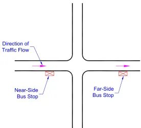
far-side bus stops. Figure 1 illustrates the difference between near-side and far-side bus
Direction of Traffic Flow
Near-Side Bus Stop
Far-Side Bus Stop
Figure 1. Diagram of Near-Side and Far-Side Bus Stops
His research presented a set of analytical equations, based on the bus stop
location, to be used instead of the traditional calculation method using Fbb to calculate
saturation flow rate adjustment factors. He simulated a CORSIM network with a two-lane
intersection approach with a curbside bus stop. In his analysis one of his network lanes
contained buses stopping and the other lane contained no buses stopping. By extracting
data from the lane with no buses stopping and applying it to the equations presented he
predicted the saturation flow rate and compared that with data obtained from the lane
with bus stops.
His research concluded that the proportion of right-turning vehicles, the distance
of the bus stop from the intersection, and the number of stopping buses had a direct effect
on the saturation flow rate. He suggested that new methods should be used to calculate
the effects of bus stops and that those methods should take into consideration the location
of the bus stop.
Recognizing the importance of Holt’s study and the methods his study contained,
this author decided to continue Holt’s research with a few modifications made to the
research methods. This author felt that by making changes to the analysis a stronger case
made was to utilize a one-way approach segment with only one travel lane. By using this
one-lane approach setup, CORSIM will not be able to allow vehicles to change lanes and
pass the bus while the bus is making a stop. Although Holt did not mention in his study if
vehicle passing did occur, this may have affected the saturation flow rate being measured.
Also, because the approaching lane will be only one lane, a comparison will not be made
between two lanes, one containing buses and one containing no buses; it will instead be
made between two networks, one containing stopping buses and one containing no
stopping buses. With these changes made this research will attempt to determine the
effects of bus stops on the saturation flow rate at signalized intersections.
Literature Review Conclusions
Holt, Rodriquez-Seda and Benekohal, and Wong et. al. all suggested that the
HCM 2000 is inadequate for predicting the effects of bus stops. Therefore, a need exists
to verify what exactly the effects are. In all three of studies, new methods were suggested
taking into account several factors concerning the buses stopping, the surrounding traffic
stream, and nearby traffic signals. This research will also seek to use similar aspects of
nearby traffic and intersection parameters in order to predict bus stop effect.
The suggestion by Rodriquez-Seda and Benekohal that the effects of a bus stop
are a function of when the bus stop arrives and departs in the cycle is interesting. Because
the signal phases control traffic flow through the intersection and buses can stop anytime
within the phases it seems logical to conclude that the time of bus stop within the cycle
plays a large part in the effect of the bus stop. Holt also made a similar assumption.
Koshy and Arasan showed the effects of micro simulation when modeling the effects of
bus stops. They asserted that micro-simulation can accurately predict the effects of bus
stops and the same assertion will be made in this study.
It is also important to note that none of the literature examined the effect of
far-side bus stops or far-side street bus stops. The Rodriquez-Seda and Benekohal and Wong et.
al. studies only examined near-side bus stops, and although the HCM mentions both
near-side and far-side bus stops it does not distinguish between the two in its calculations.
research. As part of this research, distinctions between the bus stop types will be made
CHAPTER 3 - METHODOLOGY
As explained in the Literature Review chapter, current research does not
adequately cover the effects of bus stops on the saturation flow rates of signalized
intersections. The current method in the HCM 2000 uses inconsistent dwell times within
separate chapters that seem unreasonable when examined, and does not take into account
bus stop location with respect to the intersection. Subsequent research by Rodriquez-Seda
and Benekohal, Wong et. al., and Holt have all realized this delinquency with the HCM
and have attempted to suggest alternative methods. None of the suggested methods
however, except for Holt’s, based their suggested methods on derived analytical
equations used to calculate a saturation flow rate adjustment factor. This method is based
on Holt’s work and seeks to expand his research.
This section of the research presents a new method for estimating the effects of
bus stops. It seeks to take into account factors such as defined time periods, bus stop type,
green time, flow rate, dwell time, bus stop location, and turning proportion of vehicles
that would influence the overall intersection operation, and use those to calculate more
accurate estimated impacts as a result of the buses. Adjustment factors, based on derived
equations, take into account these factors and are later compared with simulation. This
section aims to explain the methods and procedures used while conducting the research.
Model Formulation
Because the HCM fails to distinguish between bus stop locations, new equations
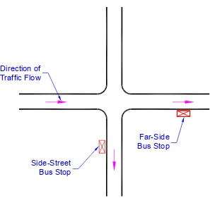
are presented for both far-side bus stops and side street bus stops. Figure 2 illustrates the
difference between far-side and side-street bus stops with relation to the approaching
Direction of Traffic Flow
Side-Street Bus Stop
Far-Side Bus Stop
Figure 2. Diagram of Far-Side and Side Street Bus Stops
Far-Side Bus Stop
A far-side bus stop is located downstream of the intersection, with respect to the
approach direction of travel. This type of bus stop requires buses to first pass through the
intersection before making their stop. Because the space available between the stopped
bus and the intersection is often limited, only a certain number of vehicles traveling in the
same lane as the bus can queue behind the bus when it is stopped.
To calculate the effects of this bus stop, several of the analytical equations and
methods in Holt’s research (5) were used, with modifications, to account for the factors
that influence bus stop effect. Some of Holt’s equations are presented below and are
borrowed from his research.
Like the equations presented by Rodriquez-Seda and Benekohal, (3) the equations
for far-side bus stops are based upon when the bus arrives within the cycle. Unlike their
research, Holt only used three time periods within the cycle to analyze bus stop effect,
account for all occurrences of a bus stopping within a signal cycle and are determined by
when the bus crosses the stop bar. Only one of the three periods occurs within any one
phase. In order to utilize these time periods we assume that traffic can only move through
the intersection in the lane group of interest during a green phase (i.e., right-turns on red
are not allowed from a shared through-right lane).
The three time periods (P1, P2, and P3) correspond to three average vehicular
volumes (V1, V2, and V3) that occur as a result of a bus crossing the stop bar during those
times. The three time periods are described as follows:
¾ P1 – Full Blockage
Time period defined by a bus arriving early enough in a green phase that it will
depart during the same phase and vehicles will be able to be processed through
the stop bar at the end of the phase. Between the time that the storage behind the
bus is filled and the bus departs, a blockage of the stop bar is created that only
ends when the bus and queue behind it moves again.
¾ P2 – Partial Blockage
Time period during the middle of a green phase in which a bus arrives and blocks
the stop bar so that it does not clear in time to process more vehicles before the
green indication ends. Any vehicles queued in the storage area behind the bus will
be released once the bus moves, but this only creates available space during the
red indication. If buses arrive during this time period, vehicles are only blocked
for part of the time between when the bus crossed the stop bar and when the bus
and queue behind it begins to move again.
¾ P3 – No Blockage
Time period at the end of a phase in which the bus arrives late enough that the
storage behind the bus never fills completely. Buses arriving during this time
period depart during the red indication. When buses arrive during this period,
there is never a blockage of approaching vehicles at the intersection.
To calculate the volume V1, during the period P1, a number of factors have to be
considered about the nature of far-side bus stops. First is the maximum number of
need for adjustment, i.e., for stopping buses. This value is referred to as the ideal number
of vehicles. If an average vehicle headway (h) is assumed, this ideal number of vehicles
can be expressed as the effective green time (g) divided by the headway, or g/h.
This study considered the stop bar on the near side of the intersection approach to
be an integral part in the calculation of the saturation flow rate due to stopping buses. The
time between the bus crossing the stop bar and starting to move again after making a stop
is referred to as the bus blockage time (BT). This blockage time can be broken down into
the time required for the bus to pass the stop bar and come to a complete stop (Ts) plus
the dwell time (Dw) required to make the stop. For the purposes of this study, both Ts and
Dw were taken from the simulation. Figure 3 illustrates the time and space relationship
between the BT and its measurement locations.
Stop Bar
Direction of
Traffic Flow Bus Stop
Begi
n Measuring
BT
(Bus Crosse
s Stop
Ba
r)
Stop Measur
ing
BT
(Bus D
eparts
from Bus Sto
p)
BT
(Bus Blockage Time)
Figure 3. Diagram of Time and Space Relationship of BT
With an understanding of BT we can then determine how the bus blocks traffic
when making a stop. If we assume that there is only a one-lane approach when a bus
stops at a curb side bus stop (or a multilane approach at saturation flow during which lane
changes are not possible), it makes sense that the traffic is blocked behind the bus and
vehicle headway, the number of vehicles blocked by the bus can be calculated by
dividing the bus blockage time by saturation headway or BT/h.
When the bus is stopped at a far-side stop there are some spaces created behind
the stop, and until those spaces are filled, traffic can continue to flow past the stop bar
through the intersection. The number of vehicles able to fill the spaces behind the bus is
directly affected by the number of vehicles turning at the intersection approach in
question and the number of vehicles on the adjacent side street turning to follow the path
of the bus on the far-side segment. Vehicles turning off of the approaching segment in
question increase the number of vehicles able to transverse the intersection, while
vehicles turning onto the bus departure segment from a side street decrease the number of
vehicles able to transverse the intersection. Considering only the vehicles turning from
the approach of interest, the number of vehicles able to traverse the intersection after the
bus crosses the stop bar can be calculated by dividing the number of storage spaces
between the bus stop and the stop bar (ST) by the proportion of through vehicles in the
traffic stream (1-Prt) or ST/(1-Prt). Figure 4 shows a diagram of the stop bar location and
the storage space for a far-side bus stop with respect to the intersection and bus stop.
Stop Bar Bus Stop
Direction of Traffic Flow Storage Spaces
(ST)
Figure 4. Diagram of Stop Bar Location and Vehicle Storage Spaces For Far-Side
The equation ST/(1-Prt) is applicable to all proportions of vehicles turning right at
the intersection. The extreme cases for this calculation are when 0% vehicles turn right at
the intersection (Prt=0) and when 100% of vehicles turn right at the intersection (Prt=1).
Examining further, if Prt = 0 and a ST value of 4 is assumed, the number of vehicles able
to traverse the intersection after the bus crosses the stop bar is equal to 4 vehicles. This
means that if 0% of vehicles turn right at the intersection, only 4 vehicles can cross the
stop bar and be stored behind the bus after the bus has crossed the stop bar.
If the other extreme case of 100% of vehicles turning right at the intersection is
examined and again a ST value of 4 is assumed, the number of vehicles able to traverse
the intersection after the bus crosses the stop bar is undefined or infinite. This calculation
result is misleading however because an infinite value of vehicles crossing after the bus is
unreasonable. Recall that the equations intended for use in calculating the number of
vehicles able to traverse an intersection after a bus, taking into consideration the
proportion of right-turning vehicles in the traffic stream. Consider that when Prt=1, there
are no vehicles traveling straight through the intersection besides the bus, and under those
circumstances this calculation is no longer needed, and can be removed from all further
saturation flow rate calculations. This extreme case though is unrealistic in itself because
it is very unlikely that a situation would exist in which only the bus would travel straight
and every other vehicle would turn right at the intersection. For the purposes of this
analysis, this extreme case was not considered because it was very unlikely to occur.
There is also a reduction in vehicles able to cross the intersection due to an
assumed lost time and startup headway delay between buses finishing their stop and
when blocked vehicles start flowing again. The lost time is due to delayed reaction time
occurring when the traffic begins to move again after a bus stop. The startup headway
delay is caused by the time incurred when blocked vehicles regain vehicle headway after
starting to move. Because delays result from both the lost time and the startup headway,
they both effectively reduce the available time for vehicles to cross the intersection. The
number of vehicles unable to traverse the intersection due to this reduction can be
calculated by adding this lost time (L) to the average headway (h) and dividing their sum
Putting all the factors together results in a calculation for the number of vehicles
processed during time period one as:
h h L P ST h
BT h g V
rt + − − + − =
1
1 (6)
This formula for flow during P1 assumes a constant maximum number of vehicles
able to be processed during the first time period. This constant assumption arises because
vehicles can traverse through the intersection both before the bus blockage time and after
the bus departs from the bus stop. Because all of the blockage time occurs during the
green time, the bus blockage time is always the same. When the blockage time is
constant, the time available to traverse the intersection is also the same, resulting in a
constant number of vehicles able to traverse the intersection.
Period one begins when the effective green time starts and doesn’t end until the
time when a bus moves past the stop bar such that a space is not created until the start of
the red time. Thus P1 can be expressed by the following boundary:
) (
0<P1 <g−BT − L+h (7)
A numerical example of the end of period one is shown by assuming a green time
of 50 sec, a bus blockage time of 25 seconds, a lost time of 2 seconds, and a vehicle
headway time of 2 seconds. The calculation is as follows:
s P of End
P of End
h L BT g P of End
21 1
) 2 2 ( 25 50 1
) ( 1
=
+ − − =
+ − − =
(8)
This example shows that 21 seconds after the start of the green time, period one
ends. At this point no more vehicles can cross the intersection without being stored
behind the bus and departing after the signal indication turns red.
The previous stated boundary of P1 assumes that g > BT + (L + h). If this
assumption is ever violated a full blockage of the traffic is never created and P1 does not
exist. In this case only P2 and P3 exist (as described below) and should be considered in
the estimation of fbb.
During the second time period (P2), buses stopping for passenger service will not
vehicles crossing through the intersection to be stored behind the bus until that space is
filled and will not allow any more vehicles to be processed through the intersection.
The number of vehicles allowed to traverse the intersection if the bus crosses the
stop bar in period two can be determined by first calculating the number of vehicles able
to cross the stop bar before the bus crosses the stop bar. This value can be represented by
dividing the time elapsed from the beginning of the green indication to when the bus
crosses the stop bar (BST) by the average vehicle headway (h) or BST/h.
By combining the number of vehicles able to traverse the intersection and fill up
available storage spaces vehicles (described previously as ST/(1-Prt)) with the number of
vehicles able to traverse the intersection before the blockage time (BST/h), we can
estimate the vehicles able to traverse the intersection when the bus crosses the stop bar
during period two as:
) 1 ( 2
rt P ST h
BST V
− +
= (9)
While this equation is the most accurate method to calculate the number of
vehicles processed as a result of buses stopping in this period, this equation is difficult to
use because very rarely is the time that the bus passes the stop bar known or able to be
measured. In its absence, the best estimation of the value V2 comes from taking an
average value of vehicles able to cross the intersection during the first time period, P1, and
the last time period, P3. During P3, as discussed later, a constant number of vehicles is
able to be processed. An alternate equation for calculating V2 is thus shown as:
2 3 1 2
V V
V = + (10)
This equation relies on the assertion that an average numbers of vehicles able to
be processed between the end of P1 and the beginning of P3 accurately reflects the number
of vehicles able to be processed during the second time period. This is true if a linear
relationship exists bridging the number of vehicles processed under P1 conditions to the
number of vehicles allowed in P3 conditions. Using equations 9 this relationship can be
illustrated by varying the time at which the bus crosses the stop bar, while holding all
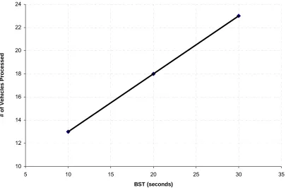
other values constant and calculating the resulting V2 values. Assuming a headway time
varying the time that the bus crosses the stop bar (BST) between 10, 20, and 30 seconds
we obtain V2 values of 13, 18, and 23 seconds, respectively. A plot of the BST versus the
number of vehicles processed is shown in Figure 5. This figure shows that the number of
vehicles processed increases at the same rate as BST during period 2, thus verifying that
the relationship between the two is linear.
10 12 14 16 18 20 22 24
5 10 15 20 25 30 35
BST (seconds)
# o
f Veh
icl
es Pro
cessed
Figure 5. Linear Relationship Between BST and the Number of Vehicles Processed
This relationship can further be explained by examining how vehicles are blocked
during this time period. Buses crossing the stop bar at the beginning of period two will
cause the storage spaces available behind the bus to fill quickly, not allowing any more
flow through the intersection. Buses crossing the stop bar at the end of this period will
allow more flow through the intersection before the bus stops and blocks traffic. Because
of this difference in trips that can be processed during certain times of the phase, the
linear relationship is present. Figure 6 is another illustration of the linear relationship
between the vehicles able to be processed and the time when the bus crosses the stop bar
#
of Proc
ess
ed
Ve
hi
cl
es
Time
V1
End of P2 (g-(St*h)/(1-Pr)) End of P1
(g-BT-(L+h))
V3
End of Green Indication
V1=g/h-BT/h+St/(1-Pr)-(L+H)
V3=(g/h)
Start of Green Indication
Period 2
Figure 6. Diagram of Time Periods and Relationships
P2 begins when the bus passes the stop bar at some time greater than g-BT-(L+h),
and ends when the bus arrives so late in the phase that the storage behind it can no longer
be filled before the light turns red. We assume that all buses depart the bus stop during
the red phase and before the start of the next green phase. This assumption is different
than that made in the Rodriquez-Seda and Benekohal study (3), which assumes that some
of the buses do not depart until after the start of the next green time.
This second period end time can be expressed as the amount of green time (g)
reduced by the amount of time required to fill up all of the storage spaces or St(h)/(1-Prt).
The numerator of this term takes into account that the storage can only be filled as fast as
the average headway (h) allows the vehicles to arrive by multiplying the storage spaces
(St) by the average headway (h). The denominator term (1- Prt) accounts for the number
of vehicles traveling straight through the intersection by subtracting the proportion of
vehicles turning right from the overall flow. Combined, the two terms calculate the time
it takes for the storage behind the bus to fill, taking into account an adjustment for
vehicles turning at the intersection.
With an understanding of the beginning and ending of time P2, the boundaries of
the time period can be expressed by:
Upper Limit P2:
rt P
h St g
− ⋅ −
1 (12)
If the difference in upper and lower limits of P2 is taken, the formula for calculating the
length of P2 can then be derived as follows:
(
)
rt rt
P h St h L BT P of Length
h L BT g P
h St g P of Length
− ⋅ − + + =
+ − − − −
⋅ − =
1 ) (
) ( 1
2 2
(13)
The P2 limits make two assumptions. The first is that g>(St(h))/(1-Prt) and the
second is that (BT+L+h)>(St(h))/(1-Prt). If either of these assumptions is violated, it
means that the storage behind the bus never completely fills. In other words, vehicles can
always be processed through the intersection and no decrease in saturation flow rate
occurs. In either of these cases, because the storage never fills, no adjustment to
saturation flow rate is needed.
During time period three (P3), the buses arrive at the stop bar and stop so late in
the green phase the available storage spaces behind the bus are never filled before the
signal turns red. Because the spaces behind the bus are never filled, the length of P3 is
directly related to the amount of time needed to fill the storage spaces behind the bus.
The third time period can therefore be calculated as:
rt P
h St P
− ⋅ =
1
3 (14)
During this time period the number of vehicles able to be processed is the same
number that would be processed assuming no bus stop took place and the traffic flow
continued through the intersection uninterrupted. The maximum number of vehicles able
to be processed when the bus crosses the stop bar during this time period is equal to the
ideal flow rate g/h and is shown as:
h g
V3 = (15)
A diagram showing the relationship of the time periods versus the maximum
amount of vehicles able to be processed was shown previously in Figure 6. With all three
time periods defined and equations for calculating length and number of vehicles derived,
estimated as the weighted average of the three time period lengths and their volumes, and
is defined as:
g P V P V P V
Vt = 1⋅ 1+ 2⋅ 2+ 3⋅ 3
(16)
This equation assumes that the bus arrives at a random time during the phase with
an equal probability of stopping during either one of the time periods.
An example of the equation applied is shown below, which assumes an approach
with a 50-second effective green time, a vehicle headway time of 2 seconds, a startup lost
time of 2 seconds, 50% of the vehicles turning right, a bus blockage time of 25 seconds,
and a storage space behind the bus of 4 vehicles.
(
)
(
)
(
) ( ) (
) ( ) ( ) ( )
[
]
bus stopping a with cycle per vehicles average V V V P h St h g P h St h l BT h g h h l P St h BT h g h l BT g h h l P St h BT h g g V t t t rt rt rt rt t 4 . 21 16 25 13 8 . 21 21 5 . 18 50 1 5 . 1 2 4 2 50 2 2 5 . 1 2 4 25 2 2 2 2 5 . 1 4 2 25 2 50 2 ) 2 2 ( 25 50 2 2 2 5 . 1 4 2 25 2 50 50 1 1 1 2 1 ) ( 1 1 = ⋅ + ⋅ + ⋅ ⎟ ⎠ ⎞ ⎜ ⎝ ⎛ = ⎥ ⎥ ⎥ ⎥ ⎥ ⎥ ⎥ ⎦ ⎤ ⎢ ⎢ ⎢ ⎢ ⎢ ⎢ ⎢ ⎣ ⎡ ⎟ ⎠ ⎞ ⎜ ⎝ ⎛ − ⋅ ⋅ ⎟ ⎠ ⎞ ⎜ ⎝ ⎛ + ⎟ ⎠ ⎞ ⎜ ⎝ ⎛ + + − ⋅ − ⋅ ⎟ ⎟ ⎟ ⎟ ⎠ ⎞ ⎜ ⎜ ⎜ ⎜ ⎝ ⎛ − + − + − ⎟ ⎠ ⎞ ⎜ ⎝ ⎛ + + − − ⋅ ⎟ ⎠ ⎞ ⎜ ⎝ ⎛ − + − + − ⎟ ⎠ ⎞ ⎜ ⎝ ⎛ = ⎥ ⎥ ⎥ ⎥ ⎥ ⎥ ⎥ ⎥ ⎦ ⎤ ⎢ ⎢ ⎢ ⎢ ⎢ ⎢ ⎢ ⎢ ⎣ ⎡ ⎟⎟ ⎠ ⎞ ⎜⎜ ⎝ ⎛ − ⋅ ⋅ ⎟ ⎠ ⎞ ⎜ ⎝ ⎛ + ⎟⎟ ⎠ ⎞ ⎜⎜ ⎝ ⎛ − ⋅ − + + ⋅ ⎟ ⎟ ⎟ ⎟ ⎠ ⎞ ⎜ ⎜ ⎜ ⎜ ⎝ ⎛ − + + − + − + + − − ⋅ ⎟⎟ ⎠ ⎞ ⎜⎜ ⎝ ⎛ − + − + − ⎟⎟ ⎠ ⎞ ⎜⎜ ⎝ ⎛ =Side-Street Bus Stops
A side-street bus stop is located on a side-street with respect to the approach
travel lane on an intersection. To access the bus stop from the approach being studied, the
bus must turn right at the intersection. This bus stop allows vehicles to queue behind the