ABSTRACT
MOORE, BRADLEY MOORE. Exploring the Impact of Value Function Uncertainty in Complex Engineered Systems. (Under the direction of Dr. Scott Ferguson).
Designing and creating complex engineering systems is a difficult proposition for engineers.
One of the frameworks proposed to help engineers with these difficulties is value driven
design. Within the framework of value driven design, a designer maps the performance of a
system to a monetary value output using a value function. However, creating correct value
functions is very difficult, often leaving the designer uncertain of the exact form. If value
driven design is going to be used by designers, the impact of this uncertainty must be known.
This thesis explores the impact of value function uncertainty through the design of two
different systems: a pressure vessel and a model rocket. The thesis first investigates how
large changes to the value functions impact the optimum solution and whether or not these
changes can be predicted. The results show that the changes can have a significant impact on
the optimum solution and that the changes to the design can sometimes be predicted. After
this, a problem is explored to identify possible solution commonalities when more realistic
uncertainty ranges are applied. Results show that when faced with uncertainty there is more
than one way to determine a best design. Designing towards the highest mean value is shown
to create systems with better performance, while designs that are immune to uncertainty have
© Copyright 2013 by Bradley Moore
Exploring the Impact of Value Function Uncertainty in Complex Engineered Systems
by
Bradley Alan Moore
A thesis submitted to the Graduate Faculty of North Carolina State University
in partial fulfillment of the requirements for the degree of
Master of Science
Aerospace Engineering
Raleigh, North Carolina
2013
APPROVED BY:
_______________________________ ______________________________ Dr. Jack Edwards Dr. Ashok Gopalarathnam
BIOGRAPHY
Bradley received his BS in Aerospace Engineering from North Carolina State
University in 2011. In undergrad, he became interested in the design of propulsion systems
and rockets. In graduate school, he spent the first semester working for Dr. Hassan studying
the ablation of heat shields. After deciding that he wanted to study design and systems
engineering he joined Dr. Ferguson’s System Design Optimization lab. In Dr. Ferguson’s lab
he joined his interests of design and rockets to conduct research in the field of Value Driven
ACKNOWLEDGMENTS
First I would like to thank Dr. Ferguson for all of his help and support through the
process of conducting this research and turning it into a thesis. I thank him for allowing me
the freedom to pick an interesting topic and explore it in a way that was very enjoyable for
me. I would also like to thank him for the many hours and late nights he spent helping me
edit and finish this document. I would like to thank my lab mates, Alex Belt, Dan Shaefer,
Garrett Foster, and Jason Denhart for keeping the many hours spent in the lab together
informative, enjoyable, and fun. I would like to thank my Mom and Dad who were always
there for me through the many struggles and hard times in my college career. Finally, I would
TABLE OF CONTENTS
LIST OF TABLES ... ix
LIST OF FIGURES ... x
Chapter 1: Introduction and Motivation ... 1
1.1 Challenges of complex system design ... 1
1.2 Current methods for complex system design ... 2
1.3 Value Driven Design ... 5
1.3.1 Value Models ... 7
1.3.2 Value Functions ... 8
1.4 Research Questions ... 9
1.4.1 Research Question 1 ... 10
1.4.2 Research Question 2 ... 11
1.5 Thesis Preview ... 11
Chapter 2: Background ... 13
2.1 Precursors to Value Driven Design ... 13
2.2 Research in Value Driven Design ... 14
2.3 Decision Making and Uncertainty in Design ... 17
Chapter 3: Solution Variability In Value Driven Design ... 20
3.1 Motivation ... 20
3.2 General Methodology ... 20
3.2.2 Value Function Types ... 21
3.2.2.1 More is Better Function ... 22
3.2.2.2 Less is Better Function ... 23
3.2.2.3 Nominal is Better Function ... 24
3.2.2.4 Piece Wise Function ... 25
3.2.3 Value Model Types ... 26
3.2.4 Testing Procedure ... 27
3.2.4.1 Using Different Value Functions ... 28
3.2.4.2 Using Different Preference Structures ... 28
3.3 Case Studies ... 28
3.3.1 Pressure Vessel: Propane Tank ... 29
3.3.1.1 Value Function Manipulation ... 33
3.3.1.2 Value Model Aggregation Structure Manipulation ... 38
3.3.2 Model Rocket ... 40
3.3.2.1 Value Function Uncertainty ... 41
3.3.2.2 Aggregation Structure Uncertainty ... 52
3.4 Results ... 57
Chapter 4: Designing Under Value Model Uncertainty ... 59
4.1 Motivation ... 59
4.2 General Methodology ... 59
4.2.1 Choosing a Baseline Value Model and Functions ... 60
4.2.3 Monte-‐Carlo Simulation ... 62
4.3 Case Study: Model Rocket ... 64
4.3.1 Model Rocket Methodology Application ... 66
4.3.1.1 Height at Apogee Performance Attribute ... 67
4.3.1.2 Flight Duration Performance Attribute ... 70
4.3.1.3 Non-‐dimensional Stability Performance Attribute ... 74
4.3.1.4 Payload Level Performance Attribute ... 76
4.4 Optimization of Model Rocket Value Under Uncertainty ... 79
4.5 Pareto Frontier Exploration ... 80
4.6 Results ... 91
Chapter 5: Conclusions and Future Work ... 96
5.1 Thesis Review ... 96
5.2 Addressing the Research Questions ... 97
5.2.1 Research Question #1: ... 98
5.2.2 Research Question #2: ... 99
5.3 Future Work ... 101
5.3.1 Different Distribution Types ... 101
5.3.2 Real Life Problem ... 101
5.4 Concluding Remarks ... 102
References ... 103
Appendix A: Functions for the Propane Tank Value Functions ... 109
LIST OF TABLES
Table 1.1: Car Design ... 3
Table 3.1: Propane Tank Variables ... 30
Table 3.2: Designer Types ... 36
Table 3.3: Model Rocket Variables ... 40
Table 3.4: Rank Ordering for Height Value Function ... 44
Table 3.5: Rank Ordering for Flight Duration Value Function ... 46
Table 3.6: Rank Ordering for Stability Value Function ... 48
Table 3.7: Payload Sizes for Model Rocket ... 49
Table 3.8: Rank Ordering for Payload Value Function ... 50
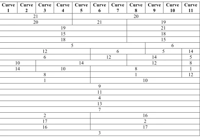
Table 3.9: Performance of Highest Value Rockets ... 56
Table 4.1: Payload Level Rocket Sizing ... 77
Table 4.2: Model Rocket Variable Bounds for MOGA ... 80
Table 4.3: Baseline Optimum Design ... 82
Table 4.4: Performance of Baseline Optimum Rocket ... 82
Table 4.5: Highest Mean Value Designs ... 83
Table 4.6: Best Mean Value Rocket Performance ... 84
Table 4.7: Smallest Standard Deviation Designs ... 84
Table 4.8: Performance of Smallest Std. Dev. Designs ... 85
Table 4.9: Middle of Frontier Designs ... 87
Table 4.10: Middle of Frontier Performance ... 87
Table 4.11: Performance of Tier 2 Rockets ... 89
Table 4.12: Performance of Tier 3 Rockets ... 90
LIST OF FIGURES
Figure 1.1: Current Large System Design Difficulties ... 2
Figure 1.2: Aircraft Value Model Hierarchy ... 7
Figure 3.1: Methodology Flow Chart ... 21
Figure 3.2: More is Better Value Function ... 23
Figure 3.3: Less is Better Value Function ... 24
Figure 3.4: Nominal is Better Value Function ... 25
Figure 3.5: Piece Wise Value Function ... 26
Figure 3.6: Pressure Vessel Model ... 30
Figure 3.7: Volume Value ($) Functions ... 32
Figure 3.8: Weight Value ($) Functions ... 32
Figure 3.9: Optimal Designs in Weight (lbs.) and Volume (gal.) for Value Function Manipulation ... 33
Figure 3.10: Risk Profiles ... 35
Figure 3.11: Designer Type Effect on Weight (lbs.) ... 36
Figure 3.12: Optimal Designs in Weight (lbs.) and Volume (gal.) for Aggregation Structure Manipulation ... 38
Figure 3.13: Volume (gal.) Preference Effect on Optimum Design ... 39
Figure 3.14: Value Functions for Height at Apogee ... 43
Figure 3.15: Value Functions for Flight Duration ... 45
Figure 3.16: Stability Value Functions ... 48
Figure 3.17: Payload Level Value Functions ... 50
Figure 3.18: Uncertain Weight Generation ... 53
Figure 3.19: Aggregation Structure Sampling ... 54
Figure 3.20: Results of Value Ranking for Weight Manipulation ... 55
Figure 4.1: Methodology Flow Chart ... 60
Figure 4.2: Generic Baseline Value Function ... 61
Figure 4.3: Generic Probability Density Function ... 63
Figure 4.4: Generated Value Functions for Generic Case ... 63
Figure 4.5: Rocket Simulator Flow Chart ... 65
Figure 4.6: Histogram of Height at Apogee Performance ... 67
Figure 4.7: Baseline Value Function for Height at Apogee ... 68
Figure 4.8: PDF for Height Value Function ... 69
Figure 4.9: Monte-Carlo Generated Height Value Functions ... 70
Figure 4.10: Histogram of Flight Duration Performance ... 71
Figure 4.11: Flight Duration Baseline Value Function ... 72
Figure 4.12: PDF for Flight Duration Value Function ... 73
Figure 4.13: Monte-Carlo Generated Flight Duration Value Functions ... 73
Figure 4.14: Baseline Stability Value Function ... 75
Figure 4.15: Monte-Carlo Generated Stability Value Functions ... 76
Figure 4.17: PDF for Value of Payload Levels ... 78
Figure 4.18: Mean Value vs. Standard Deviation of Value ... 81
Figure 4.19: Pareto Frontier Designs ... 81
Figure 4.20: Baseline and High Mean Value Rockets ... 83
Figure 4.21: Baseline and Small Std. Dev. Rockets ... 85
Figure 4.22: Middle of Pareto Frontier ... 86
Figure 4.23: Baseline and Middle Frontier Rockets ... 87
Figure 4.24: MOGA Plateau Levels ... 88
Figure 4.25: Baseline and Tier 2 Rockets ... 89
Figure 4.26: Baseline and Tier 3 Rockets ... 90
Figure 4.27: Frontier Rockets Comparison ... 94
Figure B.1: Rocket 1 ... 111
Figure B.2: Rocket 2 ... 111
Figure B.3: Rocket 3 ... 112
Figure B.4: Rocket 4 ... 112
Figure B.5: Rocket 5 ... 112
Figure B.6: Rocket 6 ... 112
Figure B.7: Rocket 7 ... 113
Figure B.8: Rocket 8 ... 113
Figure B.9: Rocket 9 ... 113
Figure B.10: Rocket 10 ... 114
Figure B.11: Rocket 11 ... 114
Figure B.12: Rocket 12 ... 114
Figure B.13: Rocket 13 ... 115
Figure B.14: Rocket 14 ... 115
Figure B.15: Rocket 15 ... 115
Figure B.16: Rocket 16 ... 116
Figure B.17: Rocket 17 ... 116
Figure B.18: Rocket 18 ... 116
Figure B.19: Rocket 19 ... 117
Figure B.20: Rocket 20 ... 117
Chapter 1:
Introduction and Motivation
1.1 Challenges of complex system design
Designing and creating large-scale systems has become more challenging as system
complexity and design team size have increased [1]. These difficulties have caused recent
government and private projects to finish over budget and behind schedule. The Boeing 787
Dreamliner, for example, was $2.5 Billion over budget and over three years late from a
delivery perspective [2]. This issue also has ramifications beyond the private sector. The
James Webb Space Telescope was initially estimated to cost $2.4 Billion and launch in 2014.
In 2008, NASA raised the price tag to $5.1 Billion, and then in 2010, the cost estimates rose
to $8.7 Billion and a launch date of 2018 [3].
Taking notice of cost overruns and delivery delays, the government executed a review
of all Department of Defense (DOD) projects since 1997. The report used the standard
provision for cost overruns in DOD projects, which is the Nunn-McCurdy provision. A
Nunn-McCurdy breach occurs when cost increases go over a certain threshold. The threshold
for a significant breach is a 15% increase over the current baseline estimate, or a 30%
increase over the original baseline estimate. Critical breaches occur when the increases are
25% over the current baseline or 50% over the original. It was discovered that since 1997
there have been 74 Nunn-McCurdy breaches, spanning 47 different defense acquisition
programs [4]. This suggests that there is a flaw with the current methodologies for large-scale
Figure 1.1: Current Large System Design Difficulties
1.2 Current methods for complex system design
Delivery delays and cost miscalculations associated with today’s complex engineered
systems may stem from the current systems engineering approach. Here, requirements are
passed down the hierarchical structure to design teams working on separate components.
Passing down requirement information leads to mistakes because there is no basic form of
comparison in overall performance between the different design teams [5]. The requirements
are set and passed down but become difficult to meet once all of the different design teams
combine their work. To explain this, consider the following hypothetical example involving a
high performance car:
1. The design team responsible for the suspension system creates a new configuration
that allows the team to decrease the weight by 50 lb. but increases the cost by $2000
due to the use of newer lightweight materials. These changes cause the design team to
come in slightly over budget, but feel that the reduction in weight warrants the
increased cost.
2. Meanwhile, a different design team working on the engine has found a way to
decrease the cost of the engine by $1800. One of the designers found that
state-of-the-art materials weren’t necessary in the cylinder heads, and slightly cheaper but heavier
heads will suffice. The engine design was already under the weight requirement, so
the team decides to use the cheaper materials. This increases the weight of the vehicle
by 75 lb.
3. Taken individually, each of these decisions seems reasonable. However, as shown in
Table 1.1, the net result is an increase in cost and weight for the car. The next
decision is crucial. A program manager could: 1) accept these changes and the
subsequent increases in cost and weight, 2) reject the changes, 3) require the two
design teams to negotiate their changes toward a neutral trade in cost and weight, or
4) pass down new requirements to each design team.
Table 1.1: Car Design
Cost Weight
Suspension design + $2000 - 50 lb.
Engine design - $1800 + 75 lb.
Net result + $200 + 25 lb.
Research into methodologies to make the design process more effective has led to
many different proposed approaches. However, many of these approaches have strength in
the qualitative realm, and significant limitations when used quantitatively. For example,
Mitsubishi first used the House of Quality in 1972 at Mitsubishi's Kobe shipyard [6]. The
House of Quality is a method that helps organize the relationships between customer needs
and what the designers can accomplish. House of Quality is a powerful tool for creating
qualitative discussion about the value of different concepts in design. However, this tool has
serious limitations when applied in a quantitative role, as it has been shown that the numbers
entered into the house are no more significant than a random process [7].
Pugh decision matrices are used in concept selection [8] by scoring the concepts in
different criteria and then totaling the score. Pugh matrices have similar limitations to House
of Quality in that they excel at facilitating qualitative discussion rather than quantitative
comparison. This is because Pugh matrices function by scoring the concepts as better or
worse when compared to a chosen datum. Yet, research has shown that this approach is
vastly subject to designer opinion and the initial choice of the datum [9]
The Analytic Hierarchical Process (AHP) is a process that was designed to help in
rational decision making by grouping concerns, components, and sub-components in a
hierarchical manner [10]. AHP is a very attractive method for choosing concepts when given
a set of alternatives. Due to how the process is set up though, it is incompatible with a set of
indefinite alternatives. This shortcoming makes it unusable inside of an optimization loop
Toward a more rigorous and mathematically sound framework, Decision Based
Design (DBD) has developed as an area of research originally presented by Hazelrigg, [11].
Decision based design is a methodology that places the design focus on the total system as
opposed to individual parts. The method does this by focusing on rational decision making
and optimizing around a single objective that represents the overall utility of a system. Using
a single objective allows the method to be used in quantitative comparisons. However, a
challenge of DBD comes in how the utility of performance attributes is modeled and how the
utilities are aggregated. This is not an inherent limitation of the method, but is more of a
modeling challenge to be addressed by the designer.
A methodology similar to decision based design is Value Driven Design or Value
based design. Value Driven Design is similar to DBD in that it recognizes the need to focus
on the optimization of a single objective. The research in this thesis focuses on Value Driven
Design and how it is used. This methodology is described in more detail in the next section.
1.3 Value Driven Design
When design concepts are compared side-by-side using performance attributes, it
becomes inherently difficult to choose the best design. This is due to the difficulty in
comparing complex systems with a large number of performance attributes. As discussed in
the previous section, there are substantial limitations to many of these approaches previously
used to make these decisions [12]. The process becomes more difficult further in the design
cycle as the designs become more similar. Value Driven Design (VDD) is a design
single metric known as “value”. Here, value is quantified in terms of a dollar amount and is
used as a measure of system “success”. The framework provides a methodology that allows
designs to be directly compared using value. VDD can be used in two different capacities
depending on how much input the designer wants within the design cycle.
The first way is to use VDD is as a “black box”, where the value model is coded into
a computer and an optimization algorithm is used to find the design with the highest possible
value. This method of operation is feasible when the system being discussed can be modeled
effectively with short simulation times. However, this approach may not be effective when
system complexity demands simulations that take hours or days to complete. If the system in
consideration is a complex system, VDD can be used as an intermediary step in the design
process.
When VDD is used as an intermediary step, simulations of the complex system are
used to estimate performance characteristics. These performances are then used to calculate
system value. Local value derivatives can then be taken with respect to the different
performance attributes to find the local gradient of the value. The local value gradient
information allows designers to know which performance attributes to focus on in their next
design iteration. Design engineers and corporations also prefer the iteration method because
the design is not completely decided by the computer algorithm.
The second manner in which VDD can be used is for calculating the worth of a new
technology [13]. When a new technology is created, it usually comes with the claim that it
will either improve performance or cut costs. The value calculation with a new technology
attributes as well as the total system value. Knowing the exact increase in value the system
shows allows the designer to see the merit of using the new technology.
1.3.1 Value Models
In order for a designer to use the VDD framework to improve the design of a system,
a value model must be created for the system. In VDD, the value model is typically created
in a hierarchical design process as shown in Figure 1.2. The figure shows a possible
hierarchy for the design of an aircraft. The total value model for the system is the
accumulation of the value of the different subsystems, which is found using the relevant
performance attributes.
Figure 1.2: Aircraft Value Model Hierarchy
A value model is the accumulation of the preferences for performance of the system
without the use of hard line requirements. In this context, preferences are viewed as an
aggregation structure for the different subsystems and performance attributes. The !"#$#%&'(%)*+'
,-#*$-*#+.'
,*/.0.-+1'(%)*+' ,*/.0.-+1'(%)*+'2#34*)."35' ,*/.0.-+1'(%)*+'!+#3605%1"$.' ,*/.0.-+1'(%)*+',-%/")"-07835-#3)'
2+#93#1%5$+' !:#"/*-+';'
2+#93#1%5$+'
!:#"/*-+'<' 2+#93#1%5$+'!:#"/*-+'=' 2+#93#1%5$+' !:#"/*-+'>'
2+#93#1%5$+' !:#"/*-+'?' 2+#93#1%5$+'
!:#"/*-+'@'
2+#93#1%5$+' !:#"/*-+'A' 2+#93#1%5$+'
preferences for the value model are compiled from the lead designer, board of directors of the
company, the client who is purchasing the system, and economic data. Due to the complex
nature of value models, there is inherently some uncertainty. This becomes clear when
looking at the hierarchy in Figure 1.2. The interaction of the subsystem value functions can
be difficult to correctly model and is a source of uncertainty in the value model. A second
source of uncertainty in the value model is in the individual performance attribute value
functions.
1.3.2 Value Functions
Value functions are the equations that translate the performance of the system in
certain attributes to gained value in dollars. The designer or design team in charge of creating
the system creates the value functions for each of the performance attributes of interest. An
example of a performance attribute is the range of an airplane. Aircraft range is a
performance attribute that would typically fall under the aerodynamics subsystem in Figure
1.2 in Section 1.3.1. The value function for range would map the possible travel distance to
value in monetary terms. This value would then be combined with the value from the other
aerodynamics performance attributes to find the subsystem value.
!"#$!!"#$%&'!()*+ =!(!"#$%,!"#$%&"'!,!"#$,!"#$,!"#.) (1.1)
The total system value is then found by combining the subsystem values within the
preference structure.
In current practice, the range of the aircraft would be given as a set minimum
requirement. Using a value function allows the designer to potentially see that even though
the airplane design may have slightly less range than the requirement, the costs go down,
which increases the overall system value.
To create a value function for a performance attribute, the general tendency of the
attributes worth must be known as a starting point. For the example of airplane range, it
might be known that an increase in range will increase the value of the plane in dollars. This
can be easily explained by the ability of the aircraft to carry a payload further without having
to refuel. A plane that can go further without refueling has a higher value in dollars. Similar
examples can be found for performance attributes where the value in dollars increases as the
attribute decreases or one where a certain nominal performance holds the highest value in
dollars [14]. Value functions can also be applied to a non-continuous performance space.
Examples of this include the ability to map value in dollars to different color patterns or
materials. Color may not be considered a normal performance attribute, but studies have
shown that color can have a very large effect on people’s willingness to buy a system [15].
1.4 Research Questions
If value driven design is going to be used in industry to help designers it must be
proven to be a reliable tool that can help designers make decisions. An important
characteristic of any design framework is that the same design will be produced given the
faith in his decisions if he knows that someone else will get the same results. This is also true
for an optimum design being similar if small changes are made to the value model.
1.4.1 Research Question 1
How sensitive is the solution from a Value Driven Design analysis, and how predictable are expected changes when changes are made to the underlying value models?
In Sections 1.2 and 1.3, the importance of value functions in VDD and the difficulty
in setting up the correct functions were described. As a designer progresses through the
design process, new information is constantly being presented. This new information can be
updates in customer preference or changes to the design mandated within the company itself,
and can lead to different value models than the one the designer started with. It is expected
that changes to the value model will cause a change in the optimum solution.
Value model uncertainty can exist in two different locations: either in the value
function or in the aggregation of the different value models. If the presence of uncertainty
impacts the optimum solution, it becomes important to understand the magnitude of the
impact and if the change can be predicted.. If a designer knows they have to make a change
to the value model, the ability to predict the change in optimum solution without rerunning
the simulation would be beneficial. It is expected that general trends in the change of the
design will be predictable, but not the exact degree of change. This is expected due to the
complex nature of the value model, and its interaction with the system model. Along with
important to figure out possible methods of making sound design decisions when faced with
uncertainty.
1.4.2 Research Question 2
When faced with uncertainty in the value model, how might the best design – or set of best designs – be determined?
The objective of VDD is to find the best system design. When the value model is
known, the criteria for finding the optimum design is that the highest value always wins.
When uncertainty is introduced into the value model, each design can have a wide variety of
value scores. This research question is designed to explore if there is a way to design the
system such that it can overcome uncertainty in the value models. Therefore, it is
hypothesized that the mean value and the standard deviation in value of a design will be
valuable metrics for finding the optimum design under uncertainty in the value model.
1.5 Thesis Preview
The questions in Section 1.4 will be investigated in the five chapters of this thesis.
Chapter 1 gives an introduction to Value Driven Design and the motivation behind the
research. Chapter 2 presents background information on decision making in engineering,
research in VDD, and designing under uncertainty. Chapter 3 and Chapter 4 investigate the
research questions and how to answer them. Chapter 3 explores the first research question
while Chapter 4 explores the second research question. Chapters 3 and 4 are broken down
studies used to test the methodologies. Chapter 5 concludes the thesis with a summary of the
Chapter 2:
Background
2.1 Precursors to Value Driven Design
As stated in the previous chapter, the research questions asked in this thesis are based
around the framework of Value Driven Design. Previous work in VDD has focused on the
creation of the framework and its application to different systems. Value driven design has
grown from the desire to have a single objective function for a design team to optimize.
Proponents of VDD believe that using a single objective function allows designers to focus
on making the correct design decision, and stems from earlier work in economics and
decision theory. Economists such as Debreu [17] stated that when presented with a choice,
the best decision is always the one with the best possible outcome. This is not directly
applicable to design however, as the outcomes are usually unknown or presented as
probabilities. Work by Von Neumann [18] attempted to overcome the uncertainty in design
by using utility lotteries and choosing the solution that presented the probability of largest
overall utility.
Herbert Simon [19] presented the idea that designers should find the optimum value
for a design, but due to computational limits believed that it was advantageous to find a less
optimum design that is easier to obtain. Simon’s idea is known as “satisficing” [20] and is
based on the idea that a designer should try to meet an acceptability threshold that may be
suboptimal. In 1977, Andrew Sage [21] built upon work performed by Keeney and Raiffa
[22], exploring decision making in large scale system design. In an effort to find optimum
Design Optimization (MDO) was formed. Work by Sobieski on integrating engineering
modeling codes into optimization structures [23] opened up the field. Cramer’s [24] work in
the field focused on how to properly set up multi-discipline engineering problems. George
Hazelrigg [11] proposed a framework for decision making in engineering design that focuses
on a single design objective. Hazelrigg’s proposal is known as Decision Based Design
(DBD), and is very similar in nature to VDD. Decision based design is presented as a method
for bringing together information and presenting it in a method to help make design
decisions.
Around the same time VDD was being presented by Collopy [5] and others, work on
Value Based Software Engineering (VBSE) was being done by Biffl et. al. [25]. VBSE is
very similar to VDD in that it focuses on making rational decisions in design, with the focus
on software rather than solid systems. After presenting VDD, Collopy continued research on
the subject, with others joining in the challenges of testing and using VDD on different
design problems.
2.2 Research in Value Driven Design
Research in the field of VDD has focused on framework implementation and
application to various design problems. After presenting the notion of VDD, Collopy then
showed how the objective functions could be created using economic-based distributed
satisfying order and transitivity properties. Potential measures of value were also presented:
surplus value, net present value, and reservation price.
One of the potential objectives, surplus value, has been used in finding the optimum
bypass ratio for a commercial plane [27]. Other work by Collopy has shown how VDD could
have saved the government $50 billion on the Joint Strike Fighter program [28]. In 2006, the
AIAA Value Driven Design committee held a workshop with the goal of applying VDD to a
government style program [29]. A value model was created for a Global Positioning System
(GPS), using the American people as the main benefactors of a GPS. This case study showed
how the process of creating a value model is carried out. Recent efforts have also focused on
how value can be used to drive the behavior of autonomous agents. Shapiro presents aligning
agent objective functions with the human user’s utility in order to create agents that more
reliably act as the user intended [30].
The inclusion of costs in a value model makes estimating part cost important in VDD.
Collopy and Eames present a new method for costing parts in aerospace systems based on the
quantity of information required to accurately make the part as opposed to older methods
based on mass or manufacturing [31]. A full review of approaches for cost modeling in the
aerospace field was performed by Curran et al. [32] by exploring contemporary cost
modeling strategies and presenting a consolidating approach called the genetic causal
approach. Technology development was explored by Hong who explored the management of
new technologies [33]. This research reviewed the manners in which programs for
Brown and Eremenko have proposed using a fractionalized approach to creating
space systems in order to increase system flexibility [34]. The idea behind the approach is to
allow the designs to adapt to uncertainty by designing the components as separate
communicating modules. A proposed method of implementing the fractionated approach is to
use a value based approach [35-37]. This approach allows for the flexibility of the
fractionated approach to be accounted for in the value model. This is significant, as Collopy
has also argued that prescribing requirements to extensive attributes, such as weight or
efficiency, severely limits the design possibilities [38].
Variations on VDD have also explored model creation for evaluating technology for
the Federal Aviation Administration (FAA) [39]. The models created in this work are very
similar to value models. Variations in metrics have also been proposed, such as probability of
success [40]. This metric is presented to replace the popular metric of ‘cost per kill’ for
military systems that has been used for fifty years.
Applications of VDD toward aircraft have included aircraft fuselage panels [41],
medium range commercial aircraft [42]., engine maintenance scheduling [43], and
aero-engines [46]. VDD was applied to two components of an aero-engine, the turbine entry
temperature and the turbine blade material. The results of the study show how when Surplus
Value Theory is applied to VDD it leads to designs that increase profit.
In 2009, Collopy reviewed different types of value models used in industry for design
optimization [16]. The work surveys and critiques some of the widely used tools for value
modeling such as Quality Function Deployment (QFD), Pugh matrices, and the Analytical
listing the steps out in order. This has also led to discussions about the differences between
Value-Centric Analysis and Value Centric Design [44], and how different architectures can
lead to different values [45]. This work found that larger multi-mission spacecraft were
fractionated into smaller simpler single mission spacecraft.
Finally, Collopy and Poleacovschi have taken the first steps in validating VDD by
setting up a program with the goal of creating a fully functioning design system complete
with simulated thinkers and design teams [47]. The continued work on this software will
allow testers to see the effects of designers changing opinions and the flow of information
between design teams and individual members during large-scale system design. This current
work also looks at validating VDD, on a simplified scale, by looking at the effects of
uncertainty within the value model.
2.3 Decision Making and Uncertainty in Design
Uncertainty is present throughout the entire design process. It can be found in
consumer preferences, designer preferences, and simulation models. Aleatory uncertainty, or
irreducible uncertainty, exists in real systems because it is inherent to the process [48]. The
effects of uncertainty on design and methods of coping with variability have been researched
using contemporary design frameworks [49], [50]. The reason for understanding uncertainty
stems from a designer’s need to make a decision when presented with incomplete
Decision-making is done in one of two ways, deterministically or
non-deterministically. The deterministic methods such as Simple Multi-Attribute Rating
Technique (SMART) [51] and value theory [52], [53] provide a way to make decisions
assuming there is no uncertainty in the model or preferences. Uncertainty is inherent in
design however, due to incomplete information or inadequate understanding.
Decision-making under uncertainty has been studied in engineering design for many years beginning
with von Neumann’s [18] utility theory. Utility theory and the axioms laid out by von
Neumann are the building block for many of the ideas and research in the field. Research in
utility theory has led to the establishment of a single attribute utility theory (SAU) and a
multi-attribute utility theory (MAU) for decision-making.
Research on uncertainty in design has focused on uncertainty existing in either the
performance of the design or the state variables that define the design. Thurston and Liu
explored uncertainty in multi-attribute utility theory by using beta distributions as probability
density functions. The beta distributions were applied to performance attributes to observe
the effect of attribute uncertainty on the desirability of alternatives [54]. Other work by
Martin and Simpson presents a method for managing uncertainty during the system-level
conceptual design [55]. The method proposes using Monte-Carlo simulation with the help of
kriging model surrogates to introduce uncertainty in the design model inputs. Work has also
been done uncertainty in decision-based design. Gurnani and Lewis created the overlap
measure method by integrating over the utility function and the probability density function
[56]. The overlap measure method allows designer to deal with uncertainty in many
Customer preferences and their uncertainty also play a very important role in decision
making for a designer. Luo et al. have proposed a methodology for designing robust systems
under consumer preference variability [57]. The proposed method uses a choice-based
conjoint analysis to elicit customer preferences and then explore their variability by looking
at the variance and covariance in the responses. The variance is then incorporated into the
design to find robust designs.
Limitations to the existing body of research are efforts exploring uncertainty in the
models being used to rate the system. These include utility functions and value models.
Pundits would argue that if there is uncertainty in the objective functions being used, then the
problem is not understood well enough. This may be the case, but unfortunately in industry
Chapter 3:
Solution Variability In Value Driven Design
3.1 Motivation
Value Driven Design is used as a tool to help engineers make decisions when
designing complex systems. As noted in 1.4.1, the selection of a value model and value
function is not an arbitrary part of the process. The value model and value functions will
decide which designs are ranked higher than others, and so must be chosen correctly. The
motivation for this chapter is to test how much solution variability exists for a system based
on changing value functions and value models. Exploring the degree of variation between
optimum solutions for a system will give insight into the solution sensitivity of VDD
analysis. The solution sensitivity of a design framework is important, because it allows the
designer to know the level of confidence with which they can present results. In decision
based design and VDD literature it is usually assumed that the preference structure and value
or utility functions are known. This is a required assumption for research focusing on the
design of a particular system. However in this work, the focus is on seeing how different, but
similar value models affect the outcome of the design process. This will give insight into how
important the accuracy of the value model is.
3.2 General Methodology
In this section, the general methodology used to find the effect of varying value
models is detailed. A flow chart of the general methodology is shown in Figure 3.1. The
method shown in Figure 3.1 is applied to two different case studies in later sections. The first
attributes and the second is a model rocket, which is a more complex problem consisting of
four performance attributes.
Figure 3.1: Methodology Flow Chart
3.2.1 Creating the Value Model and Value Functions
The framework for decision-making set forth by value driven design is motivated by
the value model and value functions. The value model and value functions are based on
economic data and designer preferences known about the system and its performance. This
requires knowledge about the performance attributes of the system and their effect on the
amount of dollars a system is worth. In this work, the value functions will be set up in a
standardized format to allow for a better understanding of the effects of either the model
preferences or value functions being altered. Here a standardized format means that the value
functions are created using the same minimum and maximum value. The differences between
the value functions exist in how the performance attribute range maps to the set value range.
3.2.2 Value Function Types
Value functions are used in VDD to relate the performance of a system into a value
score. The value score shows how much monetary value (dollars) the performance in a
particular attribute is worth. With the use of a value function, the designer does not have a set
limit, or requirement, for a particular attribute. The designer has the ability to choose a design
that might be removed if strict requirements were set because the ability to lower the
performance in one attribute allows a large gain in another, ultimately leading to a higher
overall value for the system. In this research, four different types of value functions were
used, which are detailed in Sections 3.2.2.1 – 3.2.2.4.
3.2.2.1 More is Better Function
A performance attribute can be considered “more is better” if it is known that an
increase in the attribute is better. There are multiple ways that the function can be formed,
but the general relationship must show an increase in performance leading to an increase in
value. A couple examples of attributes related to aircraft design that follow “more is better”
are the range (max travel distance) and the endurance (max time aloft). The figure below
shows three examples of how a value function that falls under “more is better” could be
Figure 3.2: More is Better Value Function
As Figure 3.2 shows, the “more is better” curve can be expressed in a multitude of
ways, as long as it follows the general trend needed. The different curves represent different
preferences a designer might have within a given performance attribute.
3.2.2.2 Less is Better Function
A second general trend for a performance attribute is one in which “less is better”. In
this case, a lower attribute score is considered better than a higher attribute score. Examples
of “less is better” for an aircraft are weight and take off distance. Figure 3.3 below shows
examples of some potential forms for “less is better”.
0 10 20 30 40 50 60 70 80 90 100
0 10 20 30 40 50 60 70 80 90 100
Performance Attribue
Value ($)
Figure 3.3: Less is Better Value Function
Similar to Section 3.2.2.1, the “less is better” trend can be expressed in a multitude of
ways, varying in nature to meet the designer’s preferences across a specific performance
attribute. The general trend is that these value functions must have a negative slope across the
performance space for an attribute.
3.2.2.3 Nominal is Better Function
The third type of value function can is set up so that a nominal value is better than
any alternative. In this case, a particular score for a performance attribute is valued higher
than the rest. The trend generally shows a positive slope before the nominal value, and then a
change in slope sign to negative above the nominal value. An example of a “nominal is
better” attribute in aircraft design is certain stability derivatives. The stability derivative
needs to be very close to a certain nominal score, with scores lower or higher than this
0 10 20 30 40 50 60 70 80 90 100
0 10 20 30 40 50 60 70 80 90 100
Performance Attribute
Value ($)
nominal score being worse. Figure 3.4 below shows some of the possible ways that a
“nominal is better” attribute curve can look.
Figure 3.4: Nominal is Better Value Function
3.2.2.4 Piece Wise Function
The fourth type of value function is a piece wise function, which can be set up to
meet the needs of a designer when none of the other methods can correctly convey the value
of an attribute. The piece wise function can also be used to show the value for discrete
attributes, such as color. Figure 3.5 below shows an example value function for a discrete
performance attribute.
0 10 20 30 40 50 60 70 80 90 100
0 10 20 30 40 50 60 70 80 90 100
Performance Attribute
Value ($)
Figure 3.5: Piece Wise Value Function
3.2.3 Value Model Types
The value model consists of the combination of all of the value functions for a given
system. A system can consist of multiple different disciplines working together such as
aerodynamics, propulsion, and structures within the development of an aircraft. The value
model sets up the connections between the different disciplines and is where the designer can
apply preference for certain performance attributes over another. The method of combination
is chosen by the designer to create the most accurate portrayal of the systems system. In this
work a weighted sum approach is used to combine the value functions. The weighted sum
approach allows all of the value functions to interact with each other as the case studies shed
complexity to avoid different teams working on different disciplines.
Typically VDD is done without using weights in the summation. The importance of
one attribute over another is contained within the value functions based on the possible range
of the value. In this work the focus is not on creating and solving a real world problem, but
rather an assessment of uncertainty in VDD. The assumption in this work of using
standardized value functions and weights creates the same effect as having value functions
Discrete 1 Discrete 2 Discrete 3 Discrete 4 Discrete 5
10 20 30 40 50 60 70 80 90 100
Performance Attribute
with different ranges. The weights serve the function of changing the scale of one
performance attribute to another, which is effectively the same as changing the range of the
value.
The basic equation that governs VDD is the following,
!"#$%($)= !"#$#"%($)− !"#$#($) (3.1)
In the case of the weighted sum approach, the equation becomes,
!"#$%!"!#$% $ = !!!![!! ∗!"#$#!"! ! −!"#$#!(!)] (3.2)
Where there are J performance attributes, X is the system design, and W is the weighting
preference for that attribute. The entire weighting preference for the model is called the
aggregation structure. The equation allows the utility (in dollars) and the costs for each
subsystem to be aggregated into the overall system value.
3.2.4 Testing Procedure
The testing procedure used in this chapter is designed around the concept of a
sensitivity study to explore how changes to the underlying value model alter the optimum
solution. This study is designed to address research question 1. The testing procedure is
broken down into two different sections. The reason for this is to separately test the effects of
using different value functions and different aggregation structures. The reason for testing the
effects separately is that it shows how each one individually impacts the optimum solution as
opposed to a combination of the multiple changes. The first step in the procedure is to
identify the important performance attributes that will be used for the study, followed by
3.2.4.1 Using Different Value Functions
1. Create a value function for each of the performance attributes.
2. Create a testing matrix for how the individual value functions will be combined in the
value model.
3. Use an aggregation structure that gives equal weighting to each of the performance
attributes.
4. Find the optimum designs for each of the combinations of value functions created in
the testing matrix.
5. Compare the optimum designs in performance space.
3.2.4.2 Using Different Preference Structures
1. Select a standard or baseline value function for each of the performance attributes.
These value functions will be used as the preference structure is altered.
2. Create a method for altering the aggregation structure ensuring the weighting
preferences add up to 100%.
3. Find the optimum designs for each of the combinations of preference weighting
structures
4. Compare the optimum design in performance space.
3.3 Case Studies
In order to test out the solution variability within VDD, two case studies were
performed. In each of these case studies, the value models and value functions were created
with two performance attributes and the second case study is a model rocket with four
performance attributes. The purpose of this is to find out how large of an effect individual
value functions and the value model can have on the optimum design output within a VDD
framework. The goal is to determine how important it is to get the value model and value
function correct when using VDD. The results from the case studies will give an
understanding of whether it is of vital importance to get the value model and value functions
correct, or if VDD is robust enough to allow for just getting the trend of the model and
functions correct. The results will also indicate whether it is possible to extrapolate certain
design trends, allowing a designer to make educated guesses about the response to a value
model or function change.
3.3.1 Pressure Vessel: Propane Tank
The first selected case study is a pressure vessel, and specifically a propane tank
designed for use on a home grill. The propane tank is being designed within the VDD
framework with two performance attributes, volume and weight. The propane tank uses three
design variables, thickness, inner radius, and length of cylindrical section. The propane tank
Figure 3.6: Pressure Vessel Model
The following table and equations show the variables and constants used in the
propane tank case study. The equations that govern the weight and volume of a 2:1 elliptical
end cap pressure vessel are from [58].
Table 3.1: Propane Tank Variables
Variables Description
Weight Total Weight of Propane Tank
Vol Volume of Propane
IR Inner Radius
T Material Thickness
L Length of Cylindrical Section
OR Outer Radius
!!"##$ = 0.283 !"#/!"#ℎ!"! Steel Density
!!"#!$%& = 4.22 !"#/!"# Propane Density
!"#$!"##$ = 0.25 !"##$%&/!" Steel Cost
!"#$!"#!$%& =3.013 !"##$%&/!"# Propane Cost
!"#$%&'()ℎ! = !(!∗!"!")!+!∗!"!∗!−!"# ∗!
!"##$ (3.4)
!"##$%&'ℎ! =!"#$%&'()ℎ!+!"#!"##$%&∗!!"#!$%& (3.5)
!"#$% $ = !!"# ∗!"#$%!"# $ +!!"#$!!∗!"#$%!"#$!! $ − !"#$($) (3.6)
The value functions show the utility in dollars (value) for each of the performance
attributes. They were created using expected performance for a typical personal use propane
tank. The first performance attribute, volume is a “more is better” type of attribute, because a
consumer will choose a design that has more propane with everything else being equal. The
volume range used in the value function is from 0 gallons to 10 gallons. Current standard
propane tanks for personal grill use are 4.7 gallons. In order to simplify the functions for ease
of comparison, the value range was set to 0 dollars for 0 gallons and 100 dollars for 10
gallons.
The range for the gallons of propane in the tank was chosen based on the minimum
weight required to produce a tank that would hold the propane without rupturing. At 10
gallons, the minimum tank weight was 80 lbs., which was chosen to be the maximum
reasonable weight. The range used does have an effect on the outcome of the study though,
as the range controls where along the value scale the typical designs fall. Ten value functions
were created for the volume performance attribute and are shown in Figure 3.7 below. The
Figure 3.7: Volume Value ($) Functions
The second performance attribute for the propane tank is the total weight, including
the weight of the propane. Weight is a “less is better” performance attribute so the functions
chosen represent this trend. The weights used to create the value function are based on the
minimum weight required to satisfy the upper and lower bounds of the volume performance
attribute. The upper bound was also tested to be a reasonable weight for someone to pick up
and possibly use. The value range was set to 0 dollars for a tank weighting 80 pounds and
100 dollars for a tank weighing 0 pounds. The value functions for weight can be seen in the
following figure with the equations being found in Appendix A.
Figure 3.8: Weight Value ($) Functions
0 0. 8 1. 6 2. 4 3. 2 4 4. 8 5. 6 6. 4 7. 2 8 8. 8 9. 6 25 50 75 100 Volume Value
0 10 20 30 40 50 60 70 80
3.3.1.1 Value Function Manipulation
Using different combinations of the value functions together tests the solution
variability of the optimum design in VDD. The first part of VDD that is necessary to look at
is how large of an effect differing value functions has on the optimum design. Ten value
functions were created for each of the performance attributes, volume and weight. For the
simulation, the weight and volume performance attributes were given equal preference in the
aggregation structure. The simulation was run with each of the ten value functions for
volume being matched with each of the ten value functions for weight. This gave a total of
one hundred optimal designs spread across the design space. This was done to find out how
many possible optimal designs there were and where they exist within the design space.
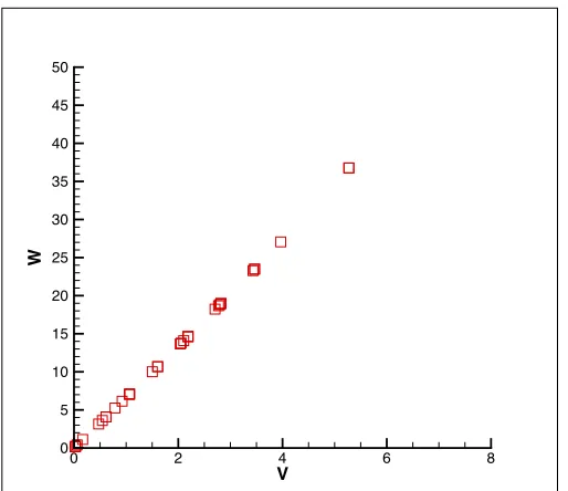
Figure 3.9: Optimal Designs in Weight (lbs.) and Volume (gal.) for Value Function Manipulation
V
W
0 2 4 6 8
The figure shows that there are a large number of different optimum designs possible
as the different value functions are used in the optimization. It is important to note that
certain designs appear more often than others. These designs are noted by the boldness of the
squares representing them. It is also interesting that designs follow a pretty linear pattern in
the performance space. The optimum designs represent the technology possible frontier of
best possible designs. The “perfect design” exists at the bottom right of the plot, having high
volume and low weight. However, due to the limitations placed on the problem not allowing
designs that will rupture, the best designs exist on this frontier. The designs, while varied due
not fill out the entire region between the lower left design and the upper right design. The
plot shows only 21 different distinct designs, whereas the simulation found optimum designs
for 100 different value function combinations.
To understand how the individual value function combinations influenced the
optimum design, the value functions were broken down as risk averse, risk neutral, or risk
prone for each of the performance attributes. Figure 3.10 shows the difference between the
different risk profiles that will be referenced from here on. The figure is for an attribute
Figure 3.10: Risk Profiles
In order to group the different risk profiles for the two performance attributes (weight
and volume) nine different designer types were created. The different designer types show
how the different value functions for each of the performance attributes affect the optimum
design. Table 3.2 below shows the breakdown for the nine different designer types. 0 10 20 30 40 50 60 70 80 90 100
0 10 20 30 40 50 60 70 80 90 100
Performance Attribute
Value ($)
Risk Neutral Risk Averse
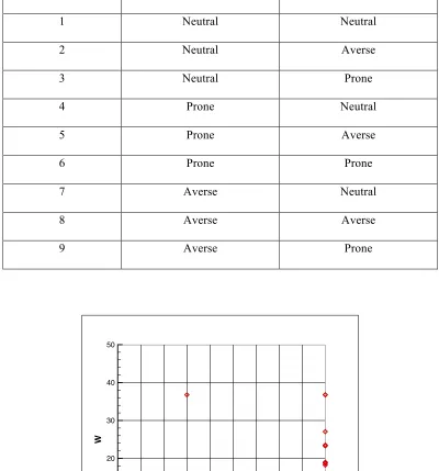
Table 3.2: Designer Types
Designer Type Volume Function Risk Type Weight Function Risk Type
1 Neutral Neutral
2 Neutral Averse
3 Neutral Prone
4 Prone Neutral
5 Prone Averse
6 Prone Prone
7 Averse Neutral
8 Averse Averse
9 Averse Prone
Figure 3.11: Designer Type Effect on Weight (lbs.)
Designer Type
W
0 1 2 3 4 5 6 7 8 9
Figure 3.11 shows how the different designer types affect the weight of the optimum
design. As the figure shows, five of the designer types have all of their designs located at the
zero weight point. The reason for this is due to the nature of the problem formulation,
specifically the maximum value being normalized to $100 for each of the performance
attributes. In this pressure vessel problem the cost is derived from the weight, thereby giving
extra incentive to drive the vessel toward a zero weight solution. For example, designer type
one is neutral for each of the performance attributes, using a linear value function. Since the
model aggregates each of the performance attributes equally in this problem, the value
formula becomes.
!"#$% $ = 0.5∗ !"#$!!"#$!!+!"#$!!"#$%& −!"#$# (3.7)
Other interesting parts of this figure to note are the designer types that have a wide
variety of weights for the optimum designs. Designer type three is risk neutral in volume and
risk prone in weight. The risk prone weight encompasses the functions below the linear
function. This means the designer is neutral towards the volume but the does not feel that
there is much value until the weight is very low. This set up leads to some designs that are
not located at the zero weight point, including the design with the highest overall volume
found for this study. The designer type that leads to all of the designs located above the zero
weight point are designer type nine. This designer type is risk averse in volume and risk
prone in weight. For this designer, having a larger than average volume is very important,
while he doesn’t attribute much value to designs unless they are low in weight. This leads to
a large range of designs that range from 6 lbs. up to 37 lbs. The next important idea to look at
3.3.1.2 Value Model Aggregation Structure Manipulation
The next important item to explore in VDD is how much of an effect changing the
aggregation structure can have on the optimal design. Changing the aggregation structure
allows the designer to change the scaling of each individual value function so that one
becomes more important than the other. For this study, a linear value function was used for
both of the performance attributes. The use of linear value functions for this study is an
arbitrary decision, and could be replaced by numerous other function forms.
Figure 3.12: Optimal Designs in Weight (lbs.) and Volume (gal.) for Aggregation Structure Manipulation
This figure shows the optimum designs, in performance space, found when the
aggregation model was altered. Similar to the study altering the value functions, there are
multiple optimum designs found when the relationship between the value functions is
V
W
0 2 4 6 8
changes. However, there is a much larger distinction between the designs in the design space,
and a lower number of unique optimum designs. As Figure 3.12 shows, there are only 8
unique designs compared to the 21 unique designs found by altering the value functions. This
occurs because there is only one value function being used for each of the performance
attributes, which does not allow for as much nuance between designs with slightly difference
performance. As the Figure 3.13 shows, there are a large number of designs at essentially the
0 weight, 0 volume location.
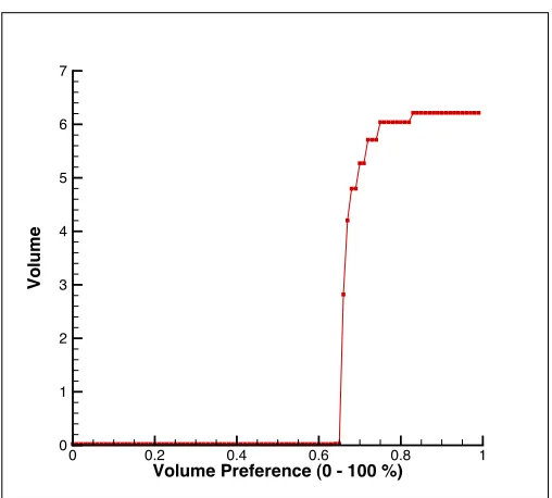
Figure 3.13: Volume (gal.) Preference Effect on Optimum Design
Figure 3.13 further shows that the optimum design stays at the zero point until the
weight applied to the volume function becomes greater than 65%. This was found to occur
due to the inclusion of cost in VDD and the manner in which it was implemented in this case Volume Preference (0 - 100 %)
Vo
lu
m
e
0 0.2 0.4 0.6 0.8 1
study. Recall that the cost was a function of the amount of material used, which becomes a
scaled restatement of the weight. It is believed that this problem is case specific as the weight
is given double the importance in the value model.
3.3.2 Model Rocket
In the second case study a more complicated problem was chosen involving the
design of a model rocket. The idea behind this problem is to make a rocket with the highest
overall value using a set rocket motor. The rocket design is based on the ability to change
eleven variables, altering the shape and materials of the different rocket parts. The rocket was
broken down into three main components: nose cone, tube body, and fins. Simplifying
assumptions made to ease the computation time were that the nose is a cone, the tube body is
the same diameter as the nose cone, and the fins are rectangular in shape with a rounded front
edge. The rocket variables are shown in Table 3.3.
Table 3.3: Model Rocket Variables
Variable Description
X-1 Rocket Diameter
X-2 Nose Cone Length
X-3 Nose Cone Thickness
X-4 Nose Cone Material
X-5 Tube Body Length
X-6 Tube Body Thickness
X-7 Tube Body Material
X-8 Fins Chord Length
X-9 Fins Height
X-10 Fins Thickness