Characterization of Traffic Flow Consumption
Pattern and Subscribers’ Behaviour
D. E. Bassey, B. E. Okon, F. O. Faith-Praise, E. E. Eyime
Senior Lecturer, Electronics and Computer Technology Unit, Department of Physics, University of Calabar, Calabar, Nigeria
Ph.D Student, Electronics and Computer Technology Unit, Department of Physics, University of Calabar, Calabar, Nigeria
Lecturer 1, Electronics and Computer Technology Unit, Dept. of Physics, University of Calabar,Calabar, Nigeria
Ph.D Student, Electronics and Computer Technology Unit, Department of Physics, University of Calabar, Calabar, Nigeria
ABSTRACT: This paper examines a series of behavioural patterns of telecommunications’ subscribers, in order to achieve better service delivery and network cost control. The use of peak values and elementary formulae used in dimensioning network elements were employed to make simple assumptions about subscriber behaviour. Printed data were coded to identify observations on low and high day control limits. Analyses of attempts from service-requests show that even when grade of service offered is satisfactory, only about 60 per cent of service-attempts were delivered to subscribers’ satisfaction. However, the obvious difference in reality is that some of these concepts when implemented do not satisfy the current subscribers’ attitude. One important features to emerge from these study is the frequency with which unsuccessful service-request are reattempted. In almost all the observations, the Grade of success was less than 0.6, and frequently less than 0.5.In addition, the grade of perseverance was not surprisingly strongly dependent onthe cause of failure. Subscribers’ calling rates vary as does their persistence in re-attempting. It is also revealing that one area which is being exploited by network operators is the deliberate manipulation of demand by the adjustment of tariff structures. Tariff schemes are designed to alter subscribers’ behavior. This affects the network’s traffic and help to smoothen out busy-hour peaks and improve the efficiency of equipment utilization. However, a balance must be achieved through deliberate policy in order to guarantee a good QoS.The study shows evidently that seasonal influences are possible. For instance, traffic increases in touristic resorts during holidays. It further noted that Call Completion Rate as a determinant for teletrafficQoS and GoS, should be reviewed as these factors do not truly certify service delivery to the satisfaction of the subscriber.
KEYWORDS: Call completion rate, Grade of service, Quality of Service, Subscribers’ behaviour, Traffic Flow.
I. INTRODUCTION
Before the explosion of digital electronics, the only way of monitoring subscribers’ behaviour was by employing personnel to observe a random sample of subscribers’ lines and to record the full details of the first call to arrive after their last observation. According to Le Gall, this method leads to an extremely biased sample of call attempts and subscribers’ behaviour; which gives a gross underestimate, in many cases of the number of unsuccessful attempts [1, 5]. Although, the time at which the attempt is observed is random, the attempts observed will not be chosen at random from all attempts. Unsuccessful repetitions tend to be bunched and omitted from the sample. However, recently, developments of high-speed electronic monitoring devices and computershave enacted a wider amount of observations to be made of all service-attempts at selected interconnection points [8].
calls handled. The number of switching nodes and links in a network depends on the number of switching devices, control devices, incoming and outgoing junctions and transmission channels [2].
In recognizing this significant role, CCITT/ITU-T structured tele-traffic domain into four major sections: Traffic modeling, Traffic performance, Dimensioning methods and Traffic measurements [1].
All subscribers of a communication network can use the services of the network at any moment of the day or night. Service usage occurs at random and independently of each other. Traffic is generated by subscribers. Not every transaction results in route occupancy or transaction; because [9]:
THE CALLED PARTY CAN BE ABSENT, THE CALLED PARTY CAN BE BUSY,
THE TRANSACTION CAN BE TERMINATED BEFORE THE PATH IS ESTABLISHED,
A CALLER CAN BE UNABLE TO ESTABLISH A CONNECTION BECAUSE NO SERVER IS FREE AT THAT MOMENT OR EQUIPMENT FAILURE. ALL THESE ATTRIBUTES CAN BE ANALYSED TO INTERPRET SUBSCRIBERS’ BEHAVIOUR.
II. RELATED WORK
Before the digital trend, simple elementary formulae used in dimensioning teletraffic networks made simple assumptions about subscribers’ behavior [4, 12]. Few examples are:
i) Full availability group: – loss system that assumes that lost calls are cleared. Each subscriber’s line has a constant calling rate when free. If a call fails, no second attempt is made.
ii) Queues at common control devices: delay system where delayed calls are assumed to wait until served. iii) Jabacus models for link system.
A. Busy Hour Call Attempts
Call attempts that are made during the peak traffic hour are busy hour call attempts (BHCA). Normally all traffic data refer to the busy hour.
Traffic, being treated by electronic microprocessors usually use call attempts per second. This refers to call attempts made during the busy hour (CAPS) [7].
CAPS = A/tm (1)
Wherein A is traffic in Erlang,
tm is average holding time of call attempts in seconds.
The relationship between CAPS and BHCA is:
CAPS = BHCA
(2) 3600 sec/hr
And
BHCA = CAPS X 3600 sec/hr (3)
B. Holding Time: In general, the call holding for a successful call is equal to the total time between the moment that the calling party picks up the service and the moment that the connection is interrupted. Holding time consists of the following:
- After lifting the service-set and the dial tone is received, the time needed to dial the number, switching time, ringing time, duration of the conversation or data/video service duration and the time needed to interrupt the connection.
For voice traffic calculations, holding time is considered to be constant [3]. Therefore, an average duration is calculated per type of voice service and per switch or network. This average voice duration refers to the arithmetic mean of the duration of a BHCA. Usually different average voice durations can be considered for voice attempts made to subscriber lines in:
- the same taxation area
- adjacent areas
- distant areas
C. Traffic:
Traffic in a network switch is the total duration of all service seizures handled by that switch. This traffic represents a time factor that can be expressed in any time unit (seconds, minute or hours). In practice, the hour (usually busy hour) is used as time unit, while traffic is expressed in Erlang.
Erlang (E, Erl) gives the total busy time of traffic sources and servers during one hour [3]. Erlang is also referred to as occupancy. A server can carry maximum of 1E. A traffic source can generate maximum of 1E. Both refer to a traffic load of 100 per cent.
The Erlang is used as the international unit for telecommunication service traffic since 1946, in memory of the Danish Mathematician, A. K. Erlang. [13]
Traffic Intensity:The quantity of traffic handled per unit time (generally the busy hour) is traffic intensity. The dimension of traffic intensity is call attempts per unit time [5].
A = Y/T = C x tm/T (4)
Where
A = traffic intensity in Erlang Y = traffic volume in Erlang-hour
C = number of busy hour call attempts (BHCA) tm = mean duration of a call attempt
D. Grade of Service
Knowledge of traffic data alone gives no indication about the service quality that the network offers. Grade of service (GoS) is a measure for the deterioration of the traffic performance of a switching system or a telecommunication network [7]. GoS of a route in a group of switching stage is the probability that a call attempt from this group will find all servers busy. GoS is a measure given from the point of view of the sufficiency of a switching equipment, referring to the probability of loss in a fault free system, or network; while the Quality of Service (QoS), refers to the network performance under error conditions. In a direct switching system configured with loss systems with infinite number of sources, a call that cannot be served is lost. The term loss probability is used and the GoS offered to subscribers is expressed by the loss probability P:
offered traffic
lost traffic
offered attempts
call
lost attempts
call
P
(5)
GOS offered
A lost A
(6)
Loss is determined by the probability of not being able to establish a connection when service attempts are made. GoS is required in any switching network to show the determined percentage allowed to be lost during the busy hour.
The permitted loss probability per switching stage or line-group in an electromechanical switch varies usually between 0.5 percent and 0.1 per cent. Digital switching systems have an extremely low loss probability (virtual non-blocking). In other networks, loss probabilities of 2 per cent to 0.5 per cent are often used (there is a trend towards lower loss probabilities in networks (GoS< 0.1per cent) [11]. Increment of the number of servers decreases the loss probability, and service quality improves.
A blocking probability of 1 per cent means that 1 per cent of traffic offered can be lost during the busy hour. The overall GoS in case of systems in series approximately equals the sum of the grade of service of each separate stage.This scenario is illustrated in Fig. 1.
FIG. 1: Link servers in series connection.
Link a
Link b
Switch a = AB – GOS = 0.01 (= 1 per cent) = Pa (7)
Switch b = BC – GOS = 0.01 (= 1 per cent) = Pb (8)
Overall loss probability = overall GOS = P
P = Pa x Pb (not mutually exclusive) (9)
1 – P = (1 – Pa) (1 – Pb) = 1 – Pa – Pb + PaPb (10)
P = Pa + Pb - PaPb (11)
Since the product, PaPb is very small, it can be neglected,
P = Pa + Pb in the example above gives:
P = 0.01 + 0.01 = 0.02 (12)
The term congestion is also used to indicate a loss probability, while time congestion is the proportion of time during which all servers are buy.
Service congestion is the proportion of the total number of service attempts that find all switches busy.
Traffic offered: The traffic value that is presented to the incoming circuits of a system or group of server is the traffic offered.
Traffic lost:Traffic that cannot be handled by the equipment or the capacity of the servers is traffic lost. Traffic that probably will be lost equals traffic offered multiplied by loss probability.
Alost = Aoff x En (Aoff) (13)
Traffic carried:Traffic that is handled by the servers is the traffic carried. The traffic carried is the traffic offered minus traffic lost:
Acan = Aoff – Acost (14)
= Aoff {1-En (Aoff)} (15)
Traffic carried per server can be considered as the efficiency: i) For loss systems, Efficiency = Acar/N (16)
Efficiency = Aoff/N is a simplification that is only meaningful in case the loss probability is low (< 3 per cent).
For routing in voice networks the route efficiency is important (60 per cent or better is usually aimed at) ii) For delay systems: Efficiency = Aoff/N (17)
(no traffic is lost in waiting systems, traffic is only delayed).
Waiting Systems
In common control configured switching systems, when a service attempt arrives when all servers are occupied, the service is delayed. The delayed service is queued until a server is free. The term delay probability or waiting probability is used:E2 (N,A) [7]
When E2 is waiting (or delay) probability
N is the number of circuits/servers A is the traffic offered in Erlang
It means delay probability, E, when traffic, A is offered to N servers. A waiting probability of 1 per cent means that a service attempt has a probability of 1 per cent delay.
III. NETWORK OBSERVATION PATTERN
This facility consists of switching system hardware, external line plant terminal of 960 subscribers interface (Subscriber Line Modules), 2,000 digital communication pots, Operation and Maintenance Terminal, a in or Plug-out terminal with Plug-output registers for Line Trunk Group Modules located in the Central Equipment room. The facility is located at the Calabar Export Processing Zone, Calabar-Nigeria. It serves both foreigners and indigenous workers. Through these devices, a deliberate step-by-step monitor of subscriber details were made for three months, and a measure of the proportion of time that all the subscriber line modules were found busy in each Line Trunk Group noted. The measurement out-put is stored in a selected register of the traffic terminal.
Call Detail Recorders, in conjunction with Artificial Traffic Generators which generate calls to various test numbers and monitor their progress were used as additional tools to access the behavioral pattern of selected subscribers. These instruments are valuable in indicating subscribers’ calling rates, holding times, traffic dispersion and observed quality of service. Traffic carried to the last choice circuit was estimated from the meter readings in the busy hour (heavy period), light period (non busy-hour period) and week-ends by using:
T=n1h (18)
Here, n1 is the LCCM reading and h the average call holding time
Or
T = n2/120 (19)
Where n2 is the LCUM reading.
Thus, the critical figures for these meters are n1 = T/h and (20)
n2=120T (21)
The EWSD–2000, switching system, used for this study routinely provides various reports without user intervention. Reports on each peak value observation was compared with control limits which are functions of the extreme engineering value distribution. Printed data were coded to identify observation on low and high day control limits. The rejection of a high day service usage by the switch is critical; and thus, the high day control limit of the switch counter was set at P (highest of N peaks > x) = 1 – PN(x) < 0.2. The counter is incremented once for each value either exceeding the 14–day peak load threshold. or the 14–day peak usage capacity which is a function of the number of facilities provided and the service criteria. For any observation lower than these the counter is decremented by one to a lower limit of zero. This standard is the universal engineering teletraffic practice that is hereby considered obsolete and may be modified in line with the findings of this study. The modification can form the basis for further studies on configuration of mega-traffic networks by stake holders.
III. RESULTS AND DISCUSSION OF OBSERVATIONS
A. Classification of Calls
Table 1, Table 2 and Table 3 give the mean values of probability of success and failure for different levels of trials for service connections with classification as indicated in each table.
Table 1: Probability of Success and Failures on Trials for Services to Subscribers within the Locality (Intra-city).
Number of trials 1Trial 2Trials 3Trials 4Trials 5 Trials Successful Service Delivery .55 .42 .39 .29 .44 Unsuccessful Service Delivery .44 .58 .61 .61 .55 Unsuccessful Service Delivery with long dist.
Blocked
.17 .29 .33 .30 .27
Unsuccessful Service Delivery with B-subscriber busy
Unsuccessful Service Delivery with A-subscriber error
.06 .05 .07 .04 .06
Unsuccessful Service Delivery without answer of B-subscriber
.09 .07 .05 .05 .07
Total Number of Trials 500
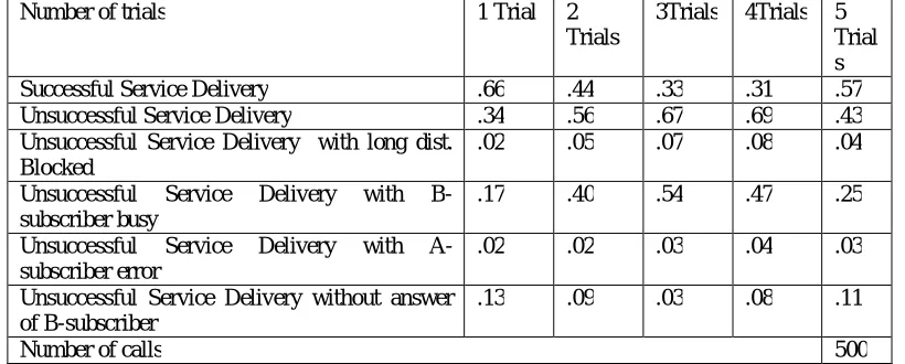
Table 2: Probability of Success and Failures on Trials for Services to Subscribers within the CEPZ Complex (Internal)
Number of trials 1 Trial 2 Trials
3Trials 4Trials 5 Trial s Successful Service Delivery .66 .44 .33 .31 .57 Unsuccessful Service Delivery .34 .56 .67 .69 .43 Unsuccessful Service Delivery with long dist.
Blocked
.02 .05 .07 .08 .04
Unsuccessful Service Delivery with B-subscriber busy
.17 .40 .54 .47 .25
Unsuccessful Service Delivery with A-subscriber error
.02 .02 .03 .04 .03
Unsuccessful Service Delivery without answer of B-subscriber
.13 .09 .03 .08 .11
Number of calls 500
Table 3: Probability of Success or Failure on Trials for Services to Intercity Subscribers (External Distance Routes) Number of trials 1Trial 2Trials 3Trials 4Trials 5Trials Successful Service Delivery .38 .33 .20 .16 .25 Unsuccessful Service Delivery .62 .67 .80 .84 .75 Unsuccessful Service Delivery with long dist. Blocked .38 .52 .59 .63 .56 Unsuccessful Service Delivery with B-subscriber busy .12 .07 .10 .13 .10 Unsuccessful Service Delivery with A-subscriber error .08 .03 .07 .03 .06 Unsuccessful Service Delivery without answer of
B-subscriber
.04 .05 .04 .05 .03
Number of calls 500
In each Table (Table 1, Table 2 and Table 3), the probability of success and failure for different reasons of failure are indicated. The probability of failure has its highest values with long distance inter-city connections and the lowest with internal connections. In each case, it increases with increment in the number of attempts; except the 5th trial, indicating release of occupied circuits as subscribers keep trying for access.B. Service Delivery for Long Distance Routes under Varying Network Congestion Period
Tables 4, 5, 6, 7 and 8 showmean values of probability of success and failure with different reasons of failure in periods of high network load, low network load and extreme high network load for long distance connections.
Table 4: Probability of Success or Failure during Periods of Heavy Load (Working Days- 8.00am to 12.00noon), Number of trials 1 trial 2 trials 3
trials
4 trials
Successful Service Delivery .44 .34 .50 .42 Unsuccessful Service Delivery with long dist blocked .31 .37 .24 .26 Unsuccessful Service Delivery with B-subscriber busy .06 .11 .07 .10 Unsuccessful Service Delivery with A-subscriber error .08 .09 .07 .10 Unsuccessful Service Delivery without answer of B-subscriber .11 .09 .12 .12
Table 5: Probability of Success or Failure during Periods of Light Load (Working Days –13.00pm to 22.00 pm) Number of trials 1trial 2 trials 3 trials 4 trials Successful Service Delivery .62 .54 .48 .37 Unsuccessful Service Delivery with long dist blocked .20 .29 .25 .28 Unsuccessful Service Delivery with B-subscriber busy .9 .11 .19 .17 Unsuccessful Service Delivery with A-subscriber error .06 .04 .02 .05 Unsuccessful Service Delivery without answer of B-subscriber .03 .02 .06 .13
No. of numbers 400
Table 6: Probability of Success and Failure during Periods of Heavy Load (week-end- 8.00hrs to18.00hrs), Number of trials 1 trial 2 trials 3 trials 4 trials Successful Service Delivery .73 .68 .57 .51 Unsuccessful Service Delivery with long dist blocked .07 .04 .09 .11 Unsuccessful Service Delivery with B-subscriber busy .13 .14 .18 .16
Unsuccessful Service Delivery with A-subscriber error .04 .05 .07 .06 Unsuccessful Service Delivery without answer of B-subscriber .03 .13 .09 .16 No. of numbers 400
Table 7: Probability of Success and Failure during Periods of Light Load (Week-end – 18.00hrs to 0800hrs) Number of trials 1 trial 2 trials 3 trials 4 trials Successful Service Delivery .78 .71 .66 .59 Unsuccessful Service Delivery with long dist blocked .03 .05 .03 .03 Unsuccessful Service Delivery with B-subscriber busy .14 .21 .23 .29 Unsuccessful Service Delivery with A-subscriber error .00 .01 .02 .02 Unsuccessful Service Delivery without answer of B-subscriber .05 .02 .06 .07
No. of numbers 400
Table 8: Probability of Success or Failure during Period of Extreme Heavy Load (Christmas day – 0800hrs to 1300hrs) Number of trials 1 trial 2 trials 3 trials 4 trials Successful Service Delivery .20 .15 .47 .34 Unsuccessful Service Delivery with long dist blocked .56 .66 .29 .45 Unsuccessful Service Delivery with B-subscriber busy .19 .10 .14 .17 Unsuccessful Service Delivery with A-subscriber error .4 .02 .03 .01 Unsuccessful Service Delivery without answer of B-subscriber .01 .07 .07 .03
No. of numbers 400
Table 9: Mean Values (secs) of Time Intervals between End of Dialling and Termination of Unsuccessful Trials.
Unsuccessful trials for local and internal connections (light load). Local calls (secs)
Long dist. Connection (secs)
Internal calls (secs) Unsuccessful Service Delivery with network blocked 2.7 - - Unsuccessful Service Delivery with B-subscriber busy 4.3 - 3.6 Unsuccessful Service Delivery with A-subscriber error 3.9 - 25.8 Unsuccessful Service Delivery without answer of B-subscriber 37.5 - 21.2 Unsuccessful Service Delivery 9.2 - 15.6 Unsuccessful Trials for Local, Long Dist., and Internal Connections(heavy load)
Unsuccessful Service Delivery with network blocked 3.3 2.6 2.3 Unsuccessful Service Delivery with B-subscriber busy 6.1 4.8 3.1 Unsuccessful Service Delivery with A-subscriber error 7.7 3.8 3.0 Unsuccessful Service Delivery without answer of B-subscriber 33.1 37.7 22.4 Unsuccessful Service Delivery 16.3 9.4 11.2
Intervals from End of Dialling to Start of Conversation:
Light load period 13.2
11.6 9.3
Heavy load period 14.8 7.6
Times of conversation
Light load period 211.0
187.3 101.3
Heavy load period 187.4 70.6
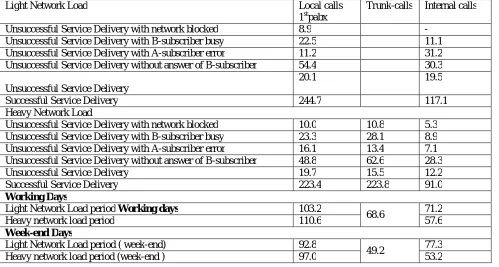
Table 10 presents the holding – times. Difference between the periods of light network load and periods of heavy network load are not significant for Unsuccessful Service Delivery with network blocked. However, for Unsuccessful Service Delivery with subscriber busy, Unsuccessful Service Delivery with A-subscriber error- and Unsuccessful Service Delivery without answer of B-subscriber calls, they are significant.
Table 10: Mean Values of Holding-times (secs)
Light Network Load Local calls 1stpabx
Trunk-calls Internal calls
Unsuccessful Service Delivery with network blocked 8.9 - Unsuccessful Service Delivery with B-subscriber busy 22.5 11.1 Unsuccessful Service Delivery with A-subscriber error 11.2 31.2 Unsuccessful Service Delivery without answer of B-subscriber 54.4 30.3
Unsuccessful Service Delivery
20.1 19.5
Successful Service Delivery 244.7 117.1 Heavy Network Load
Unsuccessful Service Delivery with network blocked 10.0 10.8 5.3 Unsuccessful Service Delivery with B-subscriber busy 23.3 28.1 8.9 Unsuccessful Service Delivery with A-subscriber error 16.1 13.4 7.1 Unsuccessful Service Delivery without answer of B-subscriber 48.8 62.6 28.3 Unsuccessful Service Delivery 19.7 15.5 12.2 Successful Service Delivery 223.4 223.8 91.0
Working Days
Light Network Load period Working days 103.2
68.6 71.2 Heavy network load period 110.6 57.6
Week-end Days
Light Network Load period ( week-end) 92.8
In the Tables presented above, some of the most interesting results obtained were analyzed. It is worth noting that two summarizing statistics can interestingly be reviewed as follows: one of the important features to emerge from these observations is the frequency with which unsuccessful service-request are reattempted.
In almost all the observations, the Grade of Success was less than 0.6, and frequently less than 0.5. The grade of perseverance was not surprisingly strongly dependent on the cause of failure. Those subscribers whose attempts failed because they met system congestion or subscriber busy tend to repeat quickly and often. Those whose attempts met subscribers who did not answer tend to abandon the service; though, there were few exceptions.
It is also revealing that one area which is being exploited by network operators is the deliberate manipulation of demand by the adjustment of tariff structures. Tariff schemes are designed to alter subscriber behavior which can affect the network: if no charge is made for service, equipment usage is maximized. If a unit rate per service is made, then, service-request times are made longer and number of service may be less than with timed service. Subscribers then increase conversation-times with the resultant burden on control equipment. If a scheme of varying charge-rates at different times is adopted, then, some traffic may be diverted from the expensive period to the cheap period; and this may help to smoothen out busy-hour peaks and improve the efficiency of equipment utilization.
The study showed evidently that seasonal influences are possible. For instance, the traffic increases in touristic resorts during holidays. This was reflected in Table 8. Telephone traffic fluctuates in the course of one day; from week to week and from season to season. It is therefore uneconomical to install so much materials in an interconnect centre as to enable it handle the highest traffic peaks. On the other hand, it is inadmissible to install only enough equipment to handle the average daily traffic density. A balance must be achieved through deliberate policy.
V. CONCLUSION
According to the study, subscribers usually re-attempt if a service-request fails before dialling is complete or if ring-tone of an engaged service-request is not obtained. Subscribers’ calling rates vary as does their persistence in reattempting. Typically, a subscriber may attempt a group of services, one after another and then make no further use of the network for a long time, or resort to network substitution. Human errors in dialling (incomplete or erroneous) and premature service disconnection without waiting for control equipment, lead to a considerable number of unsuccessful attempts. In addition, service-request which are connected to subscribers who do not answer, or to busy subscriber are usually reckoned unsuccessful for the intending subscriber; even when the call completion rate recorded successfully terminated. Call Completion Rate as a determinant for teletrafficQoS and GoS, should be reviewed as these factors do not truly certify service delivery to the satisfaction of the subscriber.
The reaction of subscribers to unsuccessful service-attempts is not the only way in which human nature impinges on the system. The study showed that all the social and economic factors in the variation of demand for the provision of satisfactory services remain unexploited; and may be too wide for this study.
REFERENCES
1. Bassey, D. E., Ogbulezie, J. C. and R. Umunnah, ‘Empirical Review of Basic Concepts of Teletraffic Postulates’, International Journal of Scientific & Engineering Research, Vol. 7 Issue 3, pp. 1171-1186, 2016.
2. Bassey, D. E., Okon, B. E. and FaithPraise, F. O., ‘Design and Construction of a GSM-Based Multipurpose Measuring Device for UHF Signal Strength Levels’, International Journal of Science, Engineering & Technology Research, Vol 5, Issue 3, pp. 841-846, 2016.
3. Bassey, D. E., Okon, B. E. and Effiom, E. O., ‘Broadband Network Penetration and Growth Pattern in North Eastern Part of Nigeria’ International Journal of Scientific & Engineering Research, Vol 7, Issue 3, pp. 1156-1170, 2016.
4. Bassey, D. E., Okoro, R. C. and Okon, B. E., ‘Issues Associated with Decimeter Waves Propagation at 0.6, 1.0 and 2.0 Peak Fresnel Zone Levels. International Journal of Science and Research Vol 5, Issue 2, pp. 159-164, 2016.
5. Bassey, D. E., Okoro, R. C. and Okon, B. E., ‘Issues of Variance of Extreme Values in a HeterogenousTeletraffic Environment’ International Journal of Science & Research, Vol 5, Issue 2, pp. 164-169, 2016.
6. Bassey, D. E., Ogbulezie, J. C. and Effiom, E. O., ‘Local Area Network (LAN) Mock-up and the Prevention of Cybernetics Related Crimes in Nigermills Company using Firewall Security Device’, International Journal of Scientific & Engineering Research, Vol 7, Issue 3, pp. 1124-1130, 2016.
7. Bassey, D. E., Ogbulezie, J. C. and Okon, B. E., ‘Modeling a Low Latency IP Network in Nigeria’ International Journal of Science, Engineering & Technology Research. Vol 5, Issue 3, pp. 830-834, 2016.
8. Bassey, D. E., Okoro, R. C. and Okon, B E., ‘Modeling of Radio Waves Transmission of Building Located around Niger Delta Urban Microcell Environment Using " Ray Tracing Techniques", International Journal of Science & Research, Vol 5, Issue 2, pp. 337-346, 2016. 9. Bassey, D. E., Okon, B. E. and Effiom, E. O., ‘Pilot Case Study of GSM - Network Load Measurement in Ikeja – Nigeria’ International
10. Bassey, D. E., Okon, B. E. and Umunnah, R., ‘The Security Implications of Virtual Local Area Network (VLAN), Niger Mills, Calabar, Nigeria’, International Journal of Scientific & Engineering Research. Vol 7, Issue 3, pp. 1187-1194, 2016.
11. Bassey, D. E and Okon, B. E., ‘Comparative Studies Between Reduction of Discrete Frequency Ranges and Radiated Sound Levels (A Case Study of 50 kVA Diesel Engine Cooling Fan’, International Journal of Engineering Research & Technology, Vol 4, Issue 9, pp. 429-437, 2016.
12. Bassey, D. E., Okoro, R. C and Ogbulezie, J. C., ‘Design Considerations of Different Segments of UHF Wireless Network in Cross River State, Nigeria’, International Journal of Science, Engineering & Technology Research, Vol 5, Issue 3, pp. 835-840, 2016.
13. Bassey, D. E., Akpan, Aniefiok O. and Udoeno, E., ‘UHF Wave Propagation Losses Beyond 40 Percent Fresnel Zone Radius in South-South Nigeria’, International Journal of Science & Research (IJSR), Vol 5, Issue 2, pp. 470-475, 2016.
14. Bassey, D. E., Okon, B. E and Effiom, E. O., ‘Pilot Case Study of GSM - Network Load Measurement in Ikeja – Nigeria’, International Journal of Science, Engineering & Technology Research, Vol 5, Issue 3, pp. 824-829, 2016.
BIOGRAPHY