University of Windsor University of Windsor
Scholarship at UWindsor
Scholarship at UWindsor
Electronic Theses and Dissertations Theses, Dissertations, and Major Papers
7-17-1969
Theoretical and experimental studies of supercritical flow over
Theoretical and experimental studies of supercritical flow over
baffles.
baffles.
M. K. Giratalla University of Windsor
Follow this and additional works at: https://scholar.uwindsor.ca/etd
Recommended Citation Recommended Citation
Giratalla, M. K., "Theoretical and experimental studies of supercritical flow over baffles." (1969). Electronic Theses and Dissertations. 6562.
https://scholar.uwindsor.ca/etd/6562
This online database contains the full-text of PhD dissertations and Masters’ theses of University of Windsor students from 1954 forward. These documents are made available for personal study and research purposes only, in accordance with the Canadian Copyright Act and the Creative Commons license—CC BY-NC-ND (Attribution, Non-Commercial, No Derivative Works). Under this license, works must always be attributed to the copyright holder (original author), cannot be used for any commercial purposes, and may not be altered. Any other use would require the permission of the copyright holder. Students may inquire about withdrawing their dissertation and/or thesis from this database. For additional inquiries, please contact the repository administrator via email
INFORMATION TO USERS
This manuscript has been reproduced from the microfilm master. UMI films
the text directly from the original or copy submitted. Thus, some thesis and
dissertation copies are in typewriter face, while others may be from any type of
computer printer.
The quality of this reproduction is dependent upon the quality of the
copy submitted. Broken or indistinct print, colored or poor quality illustrations
and photographs, print bleedthrough, substandard margins, and improper
alignment can adversely affect reproduction.
In the unlikely event that the author did not send UMI a complete manuscript
and there are missing pages, these will be noted. Also, if unauthorized
copyright material had to be removed, a note will indicate the deletion.
Oversize materials (e.g., maps, drawings, charts) are reproduced by
sectioning the original, beginning at the upper left-hand comer and continuing
from left to right in equal sections with small overlaps.
ProQuest Information and Learning
300 North Zeeb Road, Ann Arbor, Ml 48106-1346 USA 800-521-0600
NOTE TO USERS
This reproduction is the best copy available.
UMI’
THEORETICAL AND EXPERIMENTAL STUDIES
OF SUPERCRITICAL FLOW OVER BAFFLES
A THESIS
SUBMITTED TO THE FACULTY OF GRADUATE STUDIES THROUGH
THE DEPARTMENT OF CIVIL ENGINEERING IN PARTIAL
FULFILMENT OF THE REQUIREMENTS FOR THE
DEGREE OF MASTER OF APPLIED SCIENCE
AT THE UNIVERSITY OF WINDSOR
BY
M. K. GIRATALLA
WINDSOR, ONTARIO, CANADA
1969
UMI Number:EC52745
®
U M I
UMI Microform EC52745
Copyright 2007 by ProQuest Information and Learning Company. All rights reserved. This microform edition is protected against
unauthorized copying under Title 17, United States Code.
ProQuest Information and Learning Company 789 East Eisenhower Parkway
ft&QSftlS
APPROVED BY:
S', p . & 0 s 2 s z _
•5^ •
<Svs
^Ui?^
270728
ABSTRACT
A theoretical and experimental analysis of supercritical flow
over baffles is presented. Velocity distributions in the region of
dentated sills were investigated. Flow profiles were achieved by applying
the finite element method, with a systematic trial and error procedure
to adjust the free surface.
Baffle drag coefficients were calculated from experimental
readings of piezometric heads on dentated and continuous sills. Also
the drag coefficients were derived theoretically by the conformal mapping
method and numerically by the finite element method. A comparison of
drag coefficients obtained from the three independent methods, showed a
satisfactory agreement. The experimental results of drag coefficients
for dentated and continuous sills suggested the conclusion of using two
dimensional theories for the dentated sills.
Angles of deflection of the water jet measured experimentally
are compared with the deflection angles derived from conformal mapping
and those obtained from finite element method.
The conformal mapping method gave higher angles of deflection
than those obtained experimentally and theoretically by the finite element,
method, for the same ratio of the height of the impinging jet to the baffle
height.
The drag coefficients for the submerged flow previously investigated
are compared with the drag coefficients for the sweep-out condition. The
possibility of using these coefficients in determining baffle forces in the
ACKNOWLEDGEMENTS
The author wishes to express his sincere gratitude to Professor
J. A. McCorquodale (Assistant Professor of the Civil Engineering Depart
ment at the University of Windsor), under whom this thesis was written.
His suggestions, guidance and encouragement during this study and
his constructive criticism in the writing of this thesis are gratefully
acknowledged.
The financial assistance offered by the National Research
Council is greatly appreciated.
iv
TABLE OF CONTENTS
. Page
.ABSTRACT iii
.ACKNOWLEDGMENTS iv
TABLE OF CONTENTS V
LIST OF FIGURES vi-vii
LIST OF TABLES viii
.LIST OF PHOTOGRAPHS ‘ ix
CHAPTER ONE: INTRODUCTION 1
CHAPTER TWO: LITERATURE SURVEY 3
CHAPTER THREE: THEORY AND DEVELOPMENT
3.1. The Euler Equations and Conformal Mapping • . 11
3.2. Finite Element Method 18
3.3. The Relation Between Width of Flow 31
Upstream'and Between Baffles
CHAPTER FOUR: THE EXPERIMENTAL STUDY
4.1. Facilities and Equipment 33
4.2. Experimental Procedure 35
4.3. Experimental Results 36
CHAPTER FIVE: ANALYSIS AND DISCUSSION OF RESULTS
5.1. Static and Stagnation Pressures 47
5.2. Baffle Force and Drag Coefficient 49
5.3. Angle of Deflection " 5 7
CHAPTER SIX: ASSESSMENT OF ERRORS AND SCATTER IN THE EXPERIMENTAL 58 WORK
CHAPTER SEVEN: CONCLUSIONS 60
APPENDIX (I): FLOW CHARTS AND COMPUTER PROGRAMS 98
APPENDIX (II) : PHOTOGRAPHS FOR DIFFERENT FLOW CONDITIONS 117
APPENDIX (III): REFERENCES AND BIBLIOGRAPHY 125
APPENDIX (IV): NOMENCLATURE 128
LIST OF FIGURES
Figure Page
1 Flow past a plate held perpendicularly in the 15
middle of a free jet.
2 The characteristics of a triangular element 20
3 Curved boundary stream line 30
4 Flow between baffles 31
5 Schematic layout of project 38
6 Dimensions of flume'and headbox 39
7 Piezometer 40
8 Pitot tube 48
9 Illustrated plan showing the two tested transverse 48
sections (i) and (ii)
10 Distribution of piezometric taps on the upstream 50
face of the hollow baffle
11 Supercritical flow over baffle 52
12 Typical arrangement>of triangular elements 62
13-18 Flow profiles achieved by the finite element method 63-68
19-21 Variation of static and stagnation pressure 69-74
heads and the velocity in the longitudnal direction for different flow conditions.
22-24 Variation of static and stagnation pressure 75-80
heads and the velocity in the transverse direction for different flow conditions
25 Variation of pressure distribution on baffle 81
with increase of velocity of jet
26 Variation of pressure»Jdistribution on baffle 82
with increase of gate opening
27 Experimental results of drag coefficient 83
vi
28 Drag coefficient from different methods 84
29 Experimental drag coefficients for submerged 85
and sweep-out conditions
30 Experimental results of angle of deflection 86
31 Angle of deflection from different methods 87
32 Flow chart for finite element solution and 98
free surface adjustment
33 Flow chart for stifness matrix 99
34 Flow chart for assemble equations 100
35 Flow chart for solve for PSl(I$* ) 101
36 Flow chart for free surface adjustment 102
37 Flow chart for force and drag coefficient 113
List' UP TABLES
Table
1
2
3
4
5
6
7
I
8
9
10
Page
Typical values of angle of deflection (oc) against t^e 17 ratio of initial water depth to the baffle height (^) •
Observed readings of stagnation and Static Pressure 88 heads along the longitudnal centre line of flume.
Observed readings of stagnation and static pressure 89 heads in the transverse direction.
Observed readings of piezometric heads and the 90
calculated forces with their corresponding drag, coefficients for the dentated sill.
Observed readings of piezometric heads and the 92
calculated forces with their corresponding drag coefficients for the continuous sill.
Estimated values of correction factor (C^). 51
Drag coefficient (CD), and the ratio of initial 94 depth to baffle height (y/h^), for different angles of deflection (oc), by conformal mapping.
Angles of deflection, forces and drag coefficients 95 by the finite element method.
Mean, standard deviation of observations, standard 96 deviation of the mean and corrected and uncorrected means, of drag coefficients for different gate openings.
Mean, standard deviation of observations and standard 97 deviation of the mean, of angles of deflection, for different gate opening.
viii
LIST OF PHOTOGRAPHS
Photograph Page
1 Magnetic Flow Meter Chart 41
2 Side View of Equipment 42
3 Downstream View of Channel 42
4 Upstream View of the Continuous Sill 43
5 Downstream View of the Continuous Sill 44
6 View of the Pitot Tube 45
7 View of the Manometer Board 46
23 Typical Jet Profiles for Different Flow Conditions 117-124
CHAPTER ONE
INTRODUCTION
The purpose of this project is to further study the mechanics
of the forced hydraulic jump.
The velocity distributions in the vicinity of dentated sills
were studied experimentally. Static and stagnation pressure heads
in the longitudnal direction along the centre line of flume and in
the transverse direction between two baffles were measured, by means of
a pitot static tube connected to two vertical piezometer tubes. Graphs to
show the variation of velocity are plotted.
The profiles of supercritical flow over baffles were studied
:theoretically. The numerical approach in determining the flow profiles
is based on the finite element method, where the stream function at
some selected points in the region, subjected to certain boundary
conditions, are to be determined. Adjustments in the free surface
are made to make total computed energy consistent with the given
initial energy of the incoming,flow. From the finite element solution:
1) angles of jet deflection are determined; and
2) the forces on the baffle with the corresponding drag
coefficients are calculated for the different flow conditions.
The angles of deflection and drag coefficients are also determined
theoretically by the conformal mapping method, assuming no gravity and no
friction effects.
1
:The drag coefficients for both dentated and continuous sills
were obtained experimentally by measuring the piezometric pressures
-on the front and rear of one of the baffles. The forces were calcu
lated by summing the pressure forces over the normal area of the baffle.
-Actual angles of deflection of water jet were measured from photographs
•which were taken for'the different flow conditions.
The results of drag coefficients and angles of deflection obtained
from experimental results, the finite element method and conformal
— mapping are compared. Also a comparison of results of previous investi
gators is made. The possibility of using baffle drag coefficients
of supercritical flow over baffles in the forced hydraulic jump is
(Considered.
A comparison is made of the experimental results obtained from
dentated and continuous sills for different flow conditions, to check
the possibility of applying two dimensional theories to the three
dimensional flow over dentated sills. An approximate theory’ to support
CHAPTER TWO
LITERATURE SURVEY
Since the work of Bidone (l), 1820,.there has been a great increase
of knowledge pertaining to the hydraulic jump. The use of hydraulic
jump to dissipate the energy below hydraulic structures has been the
supercritical to the subcritical range causes a considerable portion
of the initial kinetic energy of the flow to be dissipated through
turbulent energy and ultimately into heat.
The effect of appurtenances such as chute blocks, baffle piers and
end sills have been used to Increase the performance of a stilling basin
to increase the dissipation of energy and reduce the required length
of the basin to prevent erosion and scouring in a natural channel section.
Bakhmeteff and Matzke (2), 1936, studied the free hydraulic.'
jump theoretically and experimentally. Their theoretical approach
used the momentum principle, which states that the rate of change
of momentum between the initial and sequential depths equals the differ
ence in hydrostatic forces, assuming that the boundary friction is
negligible. From this assumption the relation:
Their experimental work was presented in a generalized dimensionless
form, relating the kinetic flow factor 'A.', which is simply the square of accepted practice because the sudden reduction of velocity from the
1 , was developed
where: y^ — initial depth of incoming flow
y^ = sequential depth
F^ = Froude number of the incoming flow
3
the Froude number of the incoming flow, with the horizontal and vertical,
-.elements of the hydraulic jump.
• The first attempt to formulate a theory.; for forced hydraulic
jump was made by Froster and Skrinde (3), in 1950. They studied the
^forced jump formed by a sharp'-crested baffle wall and by an abrupt
i
•jrise in the floor of the channel. In the first case, a sharp crested,
aon-aerated and unsubmerged weir produced the sequent depth. A uniform
velocity distribution was assumed at the weir section. From experiments,
t r
it was found that good agreement with.theory was obtained only
•iWhen the baffle was located towards the end of the jump. For the second
case a hydrostatic pressure distribution was assumed on the abrupt
rise when the rise was situated towards the end of the jump. Fairly
good experimental correlation was obtained only when the height of rise
was relatively small.
Weaver (4) has reported interesting experiments using strain
gauges for measuring the force exerted on the baffle inside the jump.
These measurements have shown that the force exerted on a baffle wall
inside the jump decreases as the wall is moved away from the toe to a
minimum value near the end of the roller and then increases to assume
a constant value.
The second attempt at a rational solution was made by Harleman (5)
in 1955. Using the momentum equation, he developed an expression in
terms of the force exerted on the baffle piers, for calculating the
aequent depth reduction of the forced jump. He conducted experiments
on two types of baffle piers in various positions. He also measured
the force on the baffle piers by means of n device which is similar in
pointed out that the velocity is a function of the distance to the
baffles and this indicates the necessity of an analysis in which the
:drag force should be related to the flow conditions in the neighbourhood
of the baffle, rather than to that flow at the entrance section of the
stilling basin.
Bradely and Peterka (7) in 1957, summarized the work of the
United States Bureau of Reclamation in a group of six papers on the
.hydraulic design of stilling basins and their associated appurtenances.
The first paper was an academic study of the hydraulic jump on a flat
floor. The second paper covered the design of a short hydraulic jump
•stilling basin having an end sill and chute blocks. The third paper
.described a shorter stilling basin which utilizes baffle piers. This
.basin was developed for a class of smaller structures in which the
velocity at the entrance to the basin is moderate or small. The fourth
paper described a special type of hydraulic jump basin when the Froude
..number of the incoming flow is low (2.5 to 4.5). This jump produces
waves in the downstream channel. Various types of wave suppressors were devel
oped. The fifth paper described the design of a stilling basin having
a sloping apron. The last paper concerned with the design of impact
basins for large discharges and high velocities.
Moore (8) in 1957, studied the hydraulic jump and the stabilizing
1
of its position by an abrupt drop.
Rouse, Siao and Nagaratnam (9) in 1958, studied the turbulence
in the hydraulic jump by simulating the flow pattern of the jump in an
air duct and using the hot-wire anemometer to measure the corresponding
pattern of turbulence for different Froude numbers. This way, they
5
succeeded in overcoming the difficulties resulting from discontin
uities produced by entrapped air in the hydraulic jump in water.
Argyropoulos (10) in 1962, presented a generalized analysis
of hydraulic jump in sloping prismatic channels for any cross sectional
shape. The effect of the weight of water on the behaviour of the
hydraulic jump was considered, and its component in the direction
of flow was included in the analysis.
Silvester (ll) in 1964 provided exact solutions for the conju
gate depth and energy loss for hydraulic jumps in all shapes of horiz
ontal channels.
Govinda Rao and Rajaratnam (12) in 1963 presented an investigation
on the submerged hydraulic jump. They noticed that high velocities
continued along the bottom for considerable distances. Therefore they
concluded that the submerged jump was not preferred to the free jump
for energy dissipation purposes.
Later, in 1965 Rajaratnam (.13, 14) published two papers. The first
one was an attempt to solve the submerged hydraulic jump as the case
of a plane turbulent wall jet under an adverse pressure gradient over
which a backward flow has been placed. 'He, succeeded in predicting the
surface profile, velocity distribution, pressure plus momentum and energy
at any section in a given submerged jump. His second paper was an
application of the case of a plane turbulert wall jet under adverse
pressure gradient for the free hydraulic jump.
The Progress Report of the ASCE Task Force on energy dissipators for
efforts of several researchers, extended over a period of several years.
It gives a summary of discussions on the hydraulic jump and roller
bucket types of stilling basins.
Pillai and Unny (16) in 1964, studied the effect of different shapes
for appurtenances in stilling basins. They stated that blocks with an
upstream angle of 120 degrees provides best performance and help to
increase the energy dissipation and shorten length of the jump. Also
the modified shape gave less cavitation damage.
Rajaratnam (17) in 1964, developed a general theory for the forced
hydraulic jump by introducing the basin drag equation into the momentum
equation. He used seven different arrangements of baffle piers and
baffle blocks in his experimental studies. He classified the forced
jump under six major types which may be predicted either by the drag
coefficient 'CD' or by the ratio of the relative location of baffles
from the toe of the forced jump to length of the roller of the free
jump. He presented a design chart for practical design for single
baffle basin to indicate the.variation of drag coefficient with the
relative location. It was found that -the drag coefficient decreased
from about 0..1) to a minimum of 0.01 near the end of the roller, then
increasing to assume a constant value of 0.12. He also presented other
interesting studies for basins with baffle blocks, for basins with two
rows of baffles and for sunken basins.
Walter and Streeter (18) in 1964 developed a general theory for
flow over sills of various configuration in the bottom of open channels.
Methods were given for determining the velocity and pressure at any
point in the flow, as well as the location of the free surface.
7
Solutions were found by mapping conformally the planes representing
the physical flow, the complex potential and the complex velocity
onto an appropriate intermediate plane.
Rand (19, 20, 21) presented three papers on the forced hydraulic
jump. The first two papers described the flow transition in relation
ship to the boundary geometry, covering their entire physically meaningful
range. The third paper dealt with the stability of the forced hydraulic
jump and the degree of energy dissipation.
In his first paper (19) presented in 1965, he studied flow over
a vertical sill in an open channel. He concluded that such flow can be
concisely described by a set of five dimensionless variables. He also
studied the force on the sill, where he related the coefficient of drag
as a function of the Froude number, defined dimensionless variable of
the flow and the ratio of downstream depth to the initial depth. Rand
found that the drag coefficient varies from close to zero to close to
0.6, which compares well with Rajaratnam Cl?) studies oii the forced
hydraulic jump.
In his second paper (20) presented in 1966, Rand.studied the flow
over a dentated sill and concluded that the flow in this case can be
described by the same set of dimensionless variables as in the case of
continuous sill. He found that the continuous sill is the more efficient
of the two, in stabilizing the forced hydraulic jump, in reducing the
required subcritical tail water depth.and in producing a relatively
••In his third paper (21) presented in 1967,. Rand found that the
minimum possible loss over the transition length occurs at zero height
of sillji.e.j the natural jump. He found that the efficiency-of a
.forced hydraulic jump, induced by a continuous sill, in increasing the
-energy dissipation increases slightly with the Froude number and decreases
~with the increasing distance of the sill from the entrance. He noted
that the forced jump induced by the dentated sill is comparatively less
-efficient in dissipating flow energy than that induced by a continuous
one.
McCorquodale and Regts (22, 23) in (1967-68) developed a theory
. for the sequent depth of the forced hydraulic jump for a horizontal
stilling basin with a single row of baffles. The drag force was
related to the flow in the neighbourhood of the baffles. The velocity
at the baffle was determined by analysing the incoming flow as an
expanding jet. They stated, that the drag coefficient depends on the
baffle shape, the baffle height relative to the height of the impinging
jet, the baffle spacing and the Reynold's number. For fixed spacing
and shape, and for sufficiently high Reynold's number to obtain a stable
separation pattern, they developed a semi-theoretical curve, relating
the drag coefficient with the ratio of impinging flaw to the baffle
height. The two limits of their curve are as follows:
For: y ^ l ^ » 1 CD = 1.16
yb/hb = 0 CD = 2.0
Where: y^ = depth of flow just upstream the baffle
h^ = baffle height
CD = drag coefficient
9
They used a dynamometer to measure the force on the baffles. Dimension
less plots were presented to be used for design purposes.
Sweetman (24) in 1968, investigated experimentally the drag
coefficients for baffle piers in the forced hydraulic jump stilling
basin, for sweep-out and highly submerged conditions. He found that
the drag coefficients in his study follow the same trend as found by
Regts (23). Sweetman noted that for values of (y^/h^) of about 0.75
or less, the drag coefficients for sweep-out and submerged conditions
are almost the same. For (y^/li^) ) 0.75, the submerged condition
gives higher drag coefficients than the sweep-out.
Koloseus and Ahmad Daud (25) in 1969 studied the circular hydraulic
jump, i.e., the jump being circular in plan. The theoretical analysis
was based on the application of the continuity and momentum principles
to a sector of the jump. They found that the sequent depth ratio for
the same Froude number and initial depth is less for the circular
jump than that for the rectangular jump, at the same time the head loss
in a circular jump is greater than that in a rectangular jump, and the
length of the circular jump is appreciably less than the corresponding
CHAPTER THREE
THEORY AND DEVELOPMENT ■
I ' 1 ' • '
3.1. THE EULER EQUATIONS AND CONFORMAL MAPPING
Zarantonell (26) applied a theoretical method to solve problems
of a free jet of water impinging on an obstacle held vertically by
mapping conformally the planes representing, the physical flow onto an
.^appropriate intermediate plane. We note that this method is used
with the assumption that there are no gravity or friction effects.
In the case of liquid jets in air and of cavity flow, the
conformal mapping can be carried through successfully, at least in a
simple case of a horizontal free jet of water on a baffle held vertic
ally in the direction of flow, especially if the flow is rapid enough
-for gravity to be negligible and for viscosity effects to be confined
to a thin boundary layer. i.
In this case, Euler's partial differential equations for non- '
viscous flow are applicable, and one can use the free boundary conditions
of constant pressure on the liquid-gas interface to locate the free
boundary. Thus in the case of liquid jets in air, the potential theory
can be used, and P = Patm (atmospheric pressure) on the free boundary.
Zarantonell (26) summarized the conditions, under which Euler's
partial differential equations for incompressible non-viscous flow
are valid, as follows:
The vector velocity_u_is a function of vector position^• and time t, which
11 • i
possesses continuous derivatives except perhaps on exceptional surfaces
of discontinuity.
Thus in tensor notation:
■
~
(
x^
j x 2*x 3 *
— - - - - — ^ ~
^ — - - — _ C ^
A mathematically defined flow is called volume conserving or incom
pressible if and only if it satisfies the identity:
Div u ~.lL £ii za Oj for all x, t ________ [2] "S?—
i
At speeds up to 20 $ of the speed of sound (e.g. up to 220 feet per
second in air, and 950 feet per second in water), real flows are nearly
volume conserving.
Euler's equations of motion for a non-viscous, incompressible are
= _ M * p § i '__________ C3]
OXi •
Where: g = g(x) is the vector gravity
1 p = density
p .= pressure
A vector field (flow) jAx;t) is called irrotational if- it has a velocity,
potential $(xjt) whose gradient is u(x;t) so that,
u. = S<5. or u = _____________[4]
' 1 ^
Such an irrotational flow is evidently volume conserving if and only if: P' ou^
St
It is easily verified that an irrotational volume conserving
flow satisfies equation [3], if and only if the associated pressure
p(xjt) satisfies the Bernoulli's equation:
! • •
. p + .5 p 7 \§
7
$+ p. + pG = P(t) - _ ,___________ £6j,where: G = G(x) is the gravitational potential, such that g — -VG.
Such a flow, satisfying equations [4] to [6], will be called
an ideal or Euler flow.
Free Streamlines and Ideal Plane Flows:
The Bernoulli's equation [6] implies that the velocity is
constant on the boundary“for steady Euler flows ( i.e. ^ = 0,
in any steady Euler flow). Therefore, if g is negligible (i.e. if the
Froude number^=|- is sufficiently large), the two boundary conditions
are':
5$ = 0, on the fixed boundary ____________________ [7a]
dn ■
| 7 § | = constant, on the free boundary_____ __ [7b]
r
To determine complete ideal (Euler) flows satisfying equations [5],
[7a] and [7b] more advanced methods are needed. The simplest case
• is that of ideal plane flows, which is the only case in which an
extensive exact theory exists.
In plane flows, position in the physical plane may be represented
by a single complex co-ordinate Z = x + iy. The complex conjugate of
the velocity vector may be denoted by § ■+ i r\»- so thatjf =
' ! 13
and r\ ~ ~u2} w^ere ui an<* u2 are C^e va^ues obtained from equation [l]
for i = 1 and 2 respectively.
If the complex potential W is defined as § + iijf, where § is the
velocity potential and iff the stream function, then a classic result
for ideal plane flows is that W(Z) is a complex analytic function
where:
= § so that z = ,f § 1 [8]
Hence conditions [7a] and [7b] reduces to:
t|t = constant on the fixed boundary_____________________________ [8a]
dW dZ
§ I = | 4r I = constant on the free b o u n d a r y ________________ [8b]
Ideal plane flows satisfying [8], [8a] and [8b] can be found
by conformal mapping.
Circular Sector Hodographs
Zarantonell (26) stated that the mathematical theory of ideal
plane flows involves three complex quantities:
The position Z = x + iy
The complex potential W = ■§ + iljr
and the conjugate § =j£ + iT) of the complex velocity
* y, § = P "iT|
dW „ -1
We also have that : ~ = where Z = J § d W __________________[8]
The hodograph of such a flow is simply the locus of the values
-streamlines will consist of radial segments and circular arcs, centered
at § = 0.
If we assume that there is at most one stagnation point, it
.follows that flow boundary is mapped onto the boundary of a circular
sector in the hodograph plane. We can assume that this sector is
(after a change of units and co-ordinate axes)
T : 0 <; | § | £ 1 0 s; arg § £ £ _________-_________________ [9]
It is also assumed that:
i) The hodograph is simply covered (i.e., given § inside Tj there
*\ is just one point Z where the velocity is § ).
ii) Defining the W diagram of an Euler flow as the locus of all W(Z),
we shall also make the customary assumption that the W-diagram is
simply connected and simply covered.
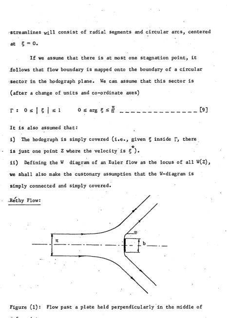
<x-Figure (l): Flow past a plate held perpendicularly in the middle of
a free jet.
15 •
Consider half the flow past a plate (of width b) held symmetrically
in a free jet of width k, as shown in Figure (l). Its W-diagram is an
infinite strip and its hodograph is a circular sector. Such a flow
is called a "Re^hy" flow.
Re'thy (26) developed an equation comprising b, n and °e in the
form:
b = 7t (1-cos =) - 2 sin o= log^ tan (^ - ~ ) _____________ ;_____ [10a]
where « is the asymptotic jet angle.
Equation [10a] can be transferred to give the relation between
the angle of deflection (cc),?and the ratio of initial water depth to
the baffle height (^), in the form:
= 1/ [ (1—cos ce ) - sin « loge tan (~ - | ) ] __________ [10b]
By assigning different values of <x3 solving to get (^), a table of
results such as shown in table (l) can be computed.
*
Refer to Selected Papers of Richard Von Mises, Volume 1, pp. 401-452
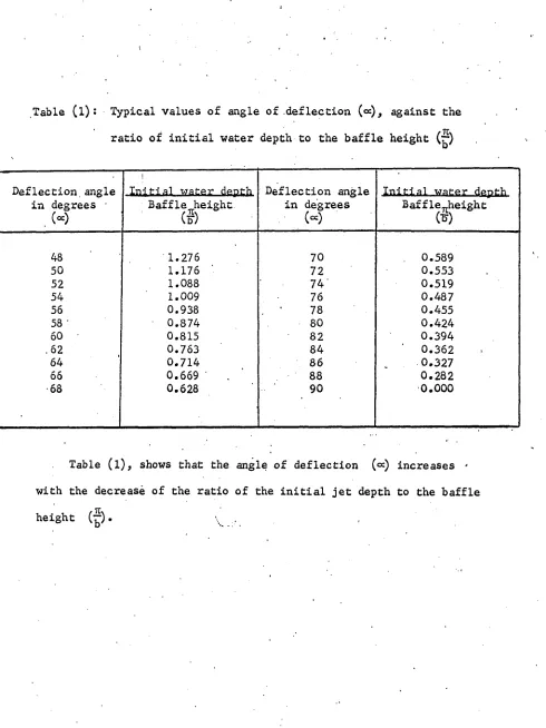
Table (l): Typical values of angle of deflection («), against the
ratio of initial water depth to the baffle height (^)
Deflection angle in degrees •
»
!
Initial water depth Deflection angle in degrees
(«)
Initial water depth Baffle height
(f)
Baffle^height
fr)
48 1.276 70 0.589
50 1.176 72 0.553
52 1.088 74' 0.519
54 1.009 76 0.487
56 0.938 78 0.455
58 ' 0.874 80 0.424
60 0.815 82 0.394
.62 0.763 84 0.362
64 0.714 86 0.327
66 0.669 ' 88 0.282
68 0.628 90 0.000
Table (l), shows that the angle of deflection («) increases *
with the decrease of the ratio of the initial jet depth to the baffle
height (^).
3.2. FINITE ELEMENT METHOD
General Remarks
One of the methods that can be used to solve the problem of super
critical flow over baffles, is the finite element method. This method
was developed originally as a concept of structural analysis (27).
However, the method is applicable to problems dealing with heat conduc
tion and fluid flow' problems. This method has been applied by
Zienkiewiez (28) in problems of seepage through porous media and irrota
tional flow of an ideal fluid, which belongs to our field of interest.
We should notice that the finite element method limits the real
system with an infinite degrees of freedom to a finite number of
degrees of freedom so that the computer solutions can be obtained.
The basic idea of the finite element formulation is the solution for
the flow field by minimizing the total kinetic energy of the system,
taking into account the boundary conditions.
The solution of such a problem is governed by a general quasi
harmonic differential equation which embraces Laplace and Poission
equations.
Theoretical Derivations
The general quasi-harmonic equation governing the behaviour of
some unknown physical quantity § can be written as:
where ;i is the unknown function assumed to be single valued within the
.>
region of the solution*
-The terms K , K , K and Q are known specified functions of x, y, zi ^ y ; * ■
f
The physical conditions of the problem impose certain boundary .
conditions, e.gi, the value of § may be specified on the boundary
Equation [ll] with the boundary conditions specifies the problem in
.a unique manner.
By the calculus of variations, we can verify that the equivalent
.formulation to equation [ll]j is the requirement that the volume
integral given in equation [12] below and taken over the whole region,
should be minimized
.X = Ky ( ^ ) 2 + K?C|J)2} - Q } > d y d * _ J _ _ [12:
For irrotational ideal two dimensional flow:
i) ' Partial derivatives with respect £0 z are zero
ii) Q = 0
iii) Kx = Ky = 1
iv) § represents the stream function =' Tjp
Therefore equation [11] reduces to
A + 1- (ft) = 0 _________ [11a]
dx 3x oy 3y
•---19
The corresponding equation to be minimized is
X = // [ .5 [(g) 2 + ( g ) 2} -] dx d y --- _ [12a]
•The procedure used to derive the necessary matrix formulation
of the problem was described by Zienkiewicz (28) and is summarized
here.
The region was divided into triangular elements or in other words
the continuum was separated by imaginary lines into a number of triang
ular finite elements. These triangular elements were assumed to be
interconnected at three discrete nodal points situated on their bound
aries.
Consider the characteristics of a triangular element. Figure (2)
shows a typical triangular element with the
nodes i, j, k numbered in an anti-clockwise
order.
If the three nodal values of define’
the function within each element, then ^
can be expresses as:
— X
t t } e
-t,
lip Figure- (2) The characteristics of a
triangular element
in the form:
ijf = a +
px
+ y Y [ 1 4 ]Then for each node, we can write
f = oc + BX. +tfY.
i * x x
= oc + SX. +'# Y.
j J J
\ = « + | 3 \ + * \
•P-^a]
[14b]
,[l4c]
Solving for °=,(3 and in terms of the nodal values i|J\, ^
and ^ by the method of determinants assuming:
1 X.
X Y.l
2A = det. 1 X.
J Yi = 2 (area of triangle i, j, k) ___ [15]
1
\ \
, il;i X.1 Y.l
^ '= det.
X . •J Y J
I I 1 1 1 1 1 1 1 1 1 1 1 t~» >—* ON
_
11x k Y k
21
A„ = det.
2
A 3 = det.
1 t. Y.
X
1 tj Y.
J
1
\
1 X.
X ' '•I*'.
1 X.
J
i|r.
1 X k
t k
[16b]
[16c]
Then: « — 1 2A
P
= t l 2A[17a]
[17b]
* = ^3
2A [17c]
Substituting the values of equations [17a], [17b] and [l7c]in
equation [14], we get finally
^ = & [(ai + biX + CiY)1i + (aj + bjX + °jY) ^ + (ak + bkX+GkY)tkJ [L8^
In which: a. — X.Y. - X Y.
i j k k j
b, = Y. - Y. = Y..
i J k jk
c = X, - X. = X, .
1 k J kj
[19a]
[19b]
[19c]
■ „ a. :+ b X 4- C.Y
Let N - l i_____ i _
a. + b.X + c.Y
N. = J J ,3
J 2A [20b]
■
k 2A
+ b, X + c, Y
k k
[20c]
Then t can be expressed in matrix form
t = CNa, Nj, Nk] Tjff
t.
t,_
.[
21]
by defining the nodal values of t throughout the region, equation
[12a] can be minimized. To achieve this we should evaluate first
the contributions of a typical element to each differential such as
5 v
dty. and then we add all such contributions and equate the differ?
f entiations to zero.
We note that only the elements adjacent to the node i will
contribute to
Equation [22] below is the differentiation of equation [12a]
with respect to t. •
a x
at. 3y' at.
23
Substituting equation [21 ] in equation [22] and arranging I
we can iwrite equation [23.].
' e ■ . ! |
^ =
T
2&)2
JT ^
^ iV bk ‘ ] W e v *
[ci*°y
cic3 £t}e
C ^ d x d y [23]For each element,, we have three differentials for the three nodes i.e.
£ f r
sxe
-ijr --- ,--- .--- C24]
'st
The final equation for one element can be written, in >a matrix
form as:
f | $ } = W ' C t J 6
_____________ :_;___________._______ [25]Where:
bibi b b j i b» b .k x c ci f Cj°i ckci
1—
1
CT
*
1
_
1
II
bibj
b.b
J j K h -k j
- i
■ ■ CiCJ Cj°j ckcjb b
A
b b k k °iCkCA
V kEquation (25) is derived for one element, to obtain the equation
of the minimization.of the whole region, we have to assemble all the
differentials of \ and equate each to zero i.e.
= T -$_X- = o
8 b ^ [27]
The summation is taken over all the elements. We note here
that, because Kx = = 1 for the whole region, the axes are the same,
for all the elements.
Slope Matrix
We are not only interested in the values of 1Jj', but also of its
gradients, which are equivalent to the components of velocity of
flow i.e.
Vy X
dx dy
-The two gradients can be developed from equation [21]-i.e.,
{grad^}
-’s j f dx
a T|r
b. . b. b.
1 . J k
c. i
1—
■ X
%
J
\
1 .
k
*
£
_
— [28]
25
Finite Element Solution and Free Surface Adjustment
A computer program to determine the stream function (i^) at some
particular points of the supercritical flow over baffle using the
finite element method, was run in the computer centre of the University
of Windsor on the IBM 360/40 computer. A systematic trial and
error solution to fix the free surface of flow was used. The compu
tation procedure was as follows:
1) For a given gate opening and discharge, the streamlines with
their values of stream function ('■jj') were assumed by choosing a
suitable trial angle of deflection. The entrance and exit
sections of the examined flow were choosen at 10.0 and 5.0 inches
respectively upstream and downstream from the baffle.
2) The region was divided into triangular elements by connecting the
adjacent nodal points. Figure (12) shows a typical arrangement
for one of the flows studied. The number of elements are forty-
nine. The number of nodal points are thirty-seven, twelve out of
i
. them are surface nodes.
3) The flow chart for the whole program is shown in figure (32),
which shows that the program could be divided into four main
parts:
A) Form Stifness Matrix: Equation (26) for each element is
l
calculated. The procedure of calculation is shown in the flow
chart figure (33). Components of velocity and the velocity
head for each element are also included in this part.
dLn the unknown Olf), equal to the number of nodal points
excluding those on the streamline or uniform flow boundaries,
-are set. The number of equations obtained was sixteen.
Procedure of calculation is shown in flow chart figure (34)
C) Solve for the unknown values of ("40 : The sixteen linear
simultaneous equations obtained in part (B) were solved to
-give the (t|f) values at the nodes not on the boundaries. An
■overrelaxation iteration method was used to solve the equations.
-The relaxation parameter (OMEGA) and tolerance factor (EPS)
were choosen as 1.5 and .00001 respectively. Steps of the
•method used are shown in flow chart figure (35).
D) The free surface was adjusted by comparing the total computed
energy at the surface elements with the known energy at the
entrance section (assuming no loss of energy in the system).
The final solution was achieved when the differences between
the computed energies at all the surface elements and the
initial energy was acceptable. Procedure of adjusting the
free surface was as follows:
i) The differences M dGn > between the computed energies at
all the surface nodes and the known energy at the entrance
section, for the assumed profile, were calculated where:
n = 1, 2, 3, . . . . L N H
LNT1 = Number of surface nodes to be adjusted;
ii) Each surface node was increased separately by an increment
(Ay), choosen as a fraction of the initial depth;
27
iii) The effect of each change of surface node (Ay), on the energy
was calculated;
iv) From calculus, we can write a set of (LNTl) simultaneous
equations of the form,
<?£, dy + !£l dy, dy [29-1]
^ 1 3y2 V Syn
and so on,
d g ^ ^ H dy + dy + + d , ... [29_n ]
^ 2 Syn
where:
dy1, dy^, . . . . dyn are the unknown first adjustments of the free
surface, and, d(^, d ^ j » • * d ^ are defined and calculated as in
step (i).
The partial derivatives (^ *) can be calculated as the rate of
change of energy differences from the true energy, as obtained from
the differences after and before applying the increment (Ay), with
respect to (Ay) e.ig.)
=
-c; - c;
SyL aYi Ay 1 [30]
where: ~ difference between the known initial energy at the
entrance section and computed energy, at the first surface node,
= difference between the known initial energy at the entrance
section and computed energy at the first surface node before applying
the increment (Ay).
A subroutine was used to solve the linear simultaneous equations
in the unknown (dy). It was based on elimination using largest pivotal
divisor. Each stage of elimination consists of interchanging rows
when necessary to avoid division by zero or small elements.
V) The new free surface is found by adding a fraction, determined
by the adjustment factor of the (dy) to the previous surface (y). If
the energy line of the new free surface is consistent with the known
initial energy, solution is complete, otherwise steps (i) to (iv)
are repeated. Procedure of adjustment is shown in flow chart figure
'(36)
The typical finite element computer programme with the free
. surface adjustment is given in Appendix I. The input data are also
shown for the various runs.
4) The program was run for three different ratios of gate opening to
baffle height. The selected ratios were 1, 3/4, 1/2. For each
ratio, two discharges were used. Figures (13 to 18) show the
final solutions obtained for the six different cases examined.
Remarks on Achieving and Improving a Convergent Solution
1) A suitable arrangement of triangular elements should be choosen.
The best arrangement appears to be that in which the elements in
regions of greatest velocities have smallest areas and vice-versa.
29
2) The convergence of the program was strongly dependent on the
choice of the deflecting angle. In other words for deflection
angles far away from the co.rrect solution} the program was
always divergent.
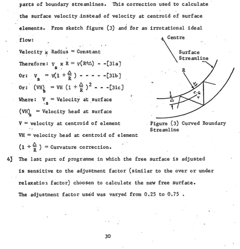
3) An improvement in the accuracy of the free surface adjustment can
be achieved if a curvature correction is applied for curved
parts of boundary streamlines. This correction used to calculate
the surface velocity .instead of velocity at centroid of surface
elements. From sketch figure (3) and for an irrotational ideal
flow:
Velocity x Radius = Constant
Therefore: v_ x R = v ( R f A ) [31a]
--- [31b] Or: V = v(l + r )
S
Or: (VH^ = VH (l + | )2 ---[31c]
Where: V = Velocity at surface -s
(VH)g = Velocity head at surface
V = velocity at centroid of element
VH = velocity head at centroid of element
A
+ Centre
Surface Streamline
Figure (3) Curved Boundary Streamline
(l + ~ ) = Curvature correction.
4} The last part of programme in which the free surface is adjusted
is sensitive to the adjustment factor (similar to the over or under
relaxation factor) choosen to calculate the new free surface.
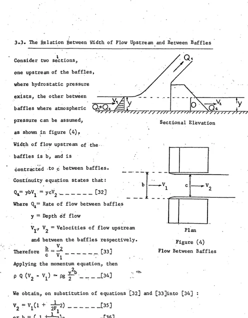
3»3. The Relation Between Width of Flow Upstream and Between Baffles
Consider two sections,
one upstream of the baffles,
where hydrostatic pressure
exists, the other between
baffles where atmospheric Q-i+Q
pressure can be assumed,
as shown in figure (4).
Width of flow upstream of the-
baffles is b, and is
contracted to c between baffles. ____
Continuity equation states that:
Qx= ybV^ = ycV2 ___________ [32]
Where Q = Rate of flow between baffles
y = Depth of flow
V^,, V2 = Velocities of flow upstream
and between the baffles respectively.
'/ / s ' s * // / // // //// //;///>//’?? / //, // / // j 'j,
Sectional Elevation
-*-V„
Therefore [33]
Plan
Figure (4)
Flow Between Baffles
Applying the momentum equation, then
2b
P Q (V2 - VL) =» pg f- _ _ _ _[34]
We obtain, on substitution of equations [32] and [33]into [34]
V = V Cl + — ^— 2}
2 1'
or b = (. 1
2F'2)c
.[35]
ir-[36]
31
For higher Froude numbers, the contraction of flow between baffles
is negligible - which means:
i) The discharge upstream the space between the baffles and the
discharge between baffles is almost the same.
ii) The discharge upstream of and over baffles is almost the same.
iii) The X-component of momentum upstream from the space between the
baffles is approximately the same as between the baffles,
From this we can conclude that the two dimensional theories
CHAPTER FOUR
THE EXPERIMENTAL STUDY
4.1. Facilities and Equipment
General Layout
The experimental part of the study of supercritical flow over
baffles was carried out in the University of Windsor Hydraulics
Laboratory. A schematic layout of the equipment is shown in figure
(5).
The flow was measured by means of a magnetic flow meter graduated
up to 2500 gallons per minute. Photograph (l) shows a view of the
magnetic flow meter chart. For discharges more than 2500 gallons
per minute, a calibrated pitot tube was used to measure the velocity
of inflow. The flow was discharged into a rectangular headbox,
where a screen was fixed between the outlet pipe and the sluice
gate to minimize the turbulence in the flume. The flow entering
the flume was regulated by an aluminum sluice gate of one foot
radius to eliminate any contraction that might occur downstream
the gate. A screw mechanism on the top of the gate, was used to
adjust the gate opening. Finally the flow was discharged through the
test section and into the sump and hence re-circulated.
Equipment
A) Flume and Headbox:
The flume and headbox were constructed from plywood with a
five feet plexiglass wall so that photographs could be taken.
Photographs (2) to (5) show views of the entire set-up. The flume was
33
placed on wooden blocks of 18 inches height. The dimensions of
the flume and headbox are shown in figure (6).
B) Baffles:
Two arrangements of baffles were examined:
i) Dentated Baffles:
Four equal baffles were attached to a movable plexiglass
floor at 65.0 centimeters from the entrance as shown in photograph
(3). Two of the four baffles were constructed from brass. One of
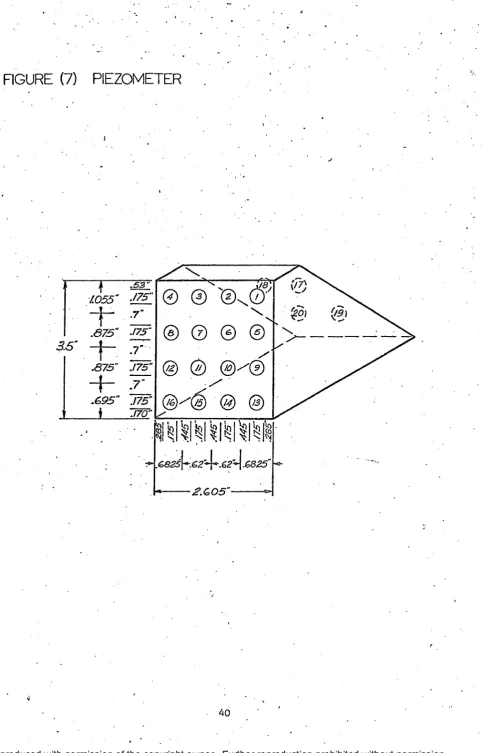
them was hollow with piezometer taps, as shown in photograph (4),
connected to the manometer board. The dimensions of the hollow
baffle with the piezometer openings are shown in figure (7). The
other brass baffle was part of a dynamometer. The other two baffles
were constructed from plexiglass,
ii) Continuous Baffle (Sill): Pieces of plywood were cut to fill
the gaps between the four baffles to constitute one continuous
baffle or sill of 3.5 inches height and 21.0 inches width (flume
width). Photographs (4) and (5) show upstream arid downstream views
of the continuous baffle. '
C) Pi tot Static Tube . . - ;
A pitot static tube of 0,12 inch external diameter and 0,046 inch
internal diameter was used to measure the stagnation and static
pressure heads in the vicinity of dentated baffles. The pitot static tube
was also used to measure velocities of inflow for discharges greater
than 2500 gallons per minute and up to 3500 gallons per minute.
The stagnation and static pressure heads were read on the vertical
D) Manometer Board
Twenty vertical piezometer tubes were attached to a graduated
plexiglass frame. Sixteen tubes were connected to the piezometer
openings in the hollow baffle to measure the pressures on the upstream
face of baffles. Two tubes were connected to the pitot static tube to measure
static and stagnation pressure heads. Photograph (7) shows a view
of the manometer board. -- •
-4.2. EXPERIMENTAL PROCEDURE
4.2.1. Static and Stagnation Pressures Measurements:
Static and stagnation pressures, in the region around the dentated
sill, were measured by means of the pitot tube. Readings were taken
at:
A) the center line between two baffles and along the longitudnal
center line of the flume at five different flow depths.
B) two sections in the transverse direction between two baffles.
The first section, with the tip of pitot tube flushes with the
upstream face of baffles, and the second with the pitot tube
one inch downstream from the first position. The measurements
were taken at the same five'flow depths used in case (A).
The pressure readings were taken for three gate openings 1.5,
^ 2.0 and 3.0 inches and discharges 1125, 1500 and 2250 gallons
per minute respectively.
35
4.2.2. Baffle Force Measurements:
The piezometric heads on the upstream face of the hollow baffle
were measured by the piezometers connected to the manometer board.
Both the dentated and continuous sills were tested.
The pressure readings were taken for nine gate openings starting
from 0.75 inch up to 4.5 inches. For each gate opening^ three different
discharges were used.
4.2.3. Angle of Deflection Measurements
The actual angle of deflection of jet was estimated from photo
graphs which were taken for different gate openings with different
discharges for the dentated and continuous sills. Some photographs
for different flow conditions are shown in Appendix II.
4.3. Experimental Results:
4.3.1. Static and Stagnation Pressures:
Table (2)* shows the observed readings of stagnation and static
pressure heads in the longitudnal direction.
Table (3), shows the observed readings of stagnation and static
pressure heads in the transverse direction.
Figures (19) to (21) show the variation of static and stagnation
pressure heads in the longitudnal direction.
Figures (22) to (24) show the variation of static arid stagnation
4.3.2* Baffle Force
Table (4) shows the observed readings of the piezometric heads
in inches of water for the dentated sill.
Table (5) shows the observed readings of the piezometric heads
in inches of water for the continuous sill.
Figure (25), shows the variation of pressure distribution on
baffle with the gate opening, at constant velocity for dentated and
continuous sills.
Figure (26), shows the variation of pressure distribution on
baffle with velocity of jet, at constant gate opening, for dentated
and continuous sills.
4.3.3. Angle of Deflection
Figure (30), shows the variation of angle of deflection (ce)
in degrees with the ratio of initial water depth to the baffle
height. Angles of deflection were estimated from photographs.
37
R e p ro d u c e d w ith p e rm is s io n of th e c o p y rig h t o w n e r. F u rt h e r re p ro d u c tio n p roh ibit ed w ith o u t p e rm is
00 s
FIGURE (5) SCHEMATIC LAYOUT OF PROJECT
PUMP
T
MAGNETIC FLOW
METER
VALVE
PITOT TUBE
FLUME
HEAD
BOX
SLUICE
GATE
\ \ V X ' \ W v T
LULU _ l CL Z i
U LlI
>< Z
9 o
CQ M
q
y
2 5 1
H
Q
Z
<
LU 2
3
Lu
Ul
O
uQ
Z
0
in
z
lu
1 Q
eg
LU
cr
Z> o
CE
U
" . . . 39 ' '
R eproduced with permission of the copyright owner. Further reproduction prohibited without permission.
S
E
C
T
IO
N
C
FIGURE (7) PIEZOMETER
3
.5
'♦
7
.055
' .53
" .175
"—j — .
7
“.
675
“ .175
“~ h .
7
“.
675
" .175
“+ - .
7
“.
0
,95
" .175
’* .
170
“\
©
©
\
\®
0
© ©
0 ® ^ ®
.&S25\~\&2 &2"\g825"
Phonograph, (l). Magnetic Ploi? Me t e r Chart
41
Photograph (2). Side V i e w of Equipmen
Photograph (3). Downstream View of Channel
Photograph (4). Upstream Viev of the Continuous Sill
43
•Photograph (5). Downstream View of the Continuoxis Sill
Photograph (6). Vie-w of the Pitot Tube
tfi <•#
45
Photograph (7). View of the Manometer Board
CHAPTER FIVE
ANALYSIS AND DISCUSSION OF RESULTS
5.1. Static and Stagnation Pressures
The variation of static and stagnation pressure heads in inches
of water at the centre line between two baffles and along the longi-
tudnal centre line of the flume for different flow conditions are
plotted in figures (19 to 21).
The velocity in feet per second at every point was calculated
from equation [37].
V - “static) ‘ 12 — --- :
Where:
1 V = velocity of flow in feet per second.
^stag = sta8nat^on Pressure head in inches of water
H _ = static pressure head in inches of water
static r
2 g = gravitational acceleration in ft./sec. .
The variation of velocity is also shown on figures (19 to 21).
We notice that:
1) The velocity at entrance and exit sections is nearly the same,
which means that there is a very little change in the X-component
of momentum of flow before and after the baffle.
. 4 7
2) The velocity just upstream of the baffle is less than the velocities
iat the entrance and exit sections. This is most likely caused by
the interference of flow as a result of the adjacent baffles.
.This phenomenon is more pronounced near the bottom of flume.
H
J
static
stag cn w rf if ft (W
H* 3
0 0>
It
H-d o
a> 3 ta 01 * 3
C ^
l-J ID
(0 CO
. 01
1 c
' s
I p
tl.5 U '
Figure (8)
Pitot Static Tube
| Flow 3) A downstream displacement of
-0.5 inch was considered in
^plotting the static pressure
heads. This displacement was
done, because the static
pressure was measured at points 0.5
inch downstream the measured stag
nation pressure, as shown in
figure (8).
The experimental results of
static and stagnation pressure
heads in the transverse direction at ,
the two sections, shorn in the
illustrated plan figure (9),
were plotted in figures (22 to 24).
The velocity of flow at every point was
calculated by equation [ 3 7 and plotted
on figures (22 to 24). These figures
show:
1) There is symmetry in the results with respect to the centre line
between the two adjacent baffles for any particular case.
Section (i
r
Section J.
(ii)
BAFFLE BAFFLE
Figure (9)
2) For the same discharge and gate opening, and at a fixed depth,
there is not much difference in velocity profiles between
the two transverse sections mentioned above.
3) Static pressure is almost constant in the transverse direction
between the two baffles for. a given discharge and gate opening,
, and at a fixed depth.
4) For the same discharge and gate opening, it was noticed that:
i) At higher depths, the stagnation pressure is almost constant
except near the two baffles, where it suddenly dropped to a
value equal or little higher than the corresponding static pressure,
which means that the velocity is almost constant between baffles •
and suddenly vanishes near the baffle walls. This indicates
that the contraction of flow path while passing between baffles
is very small.
ii) At lower depths, stagnation pressure starts increasing,
towards the baffle walls, with a decreasing rate, from its value
at centre line between the two baffles. When approaching the
baffle walls, the stagnation pressure decreases to a value equal
or little higher than the corresponding static pressure. This
means that the centre line velocity at lower depths is less than
velocities at both sides, then finally approaches zero near the
baffle walls. . • .
5.2. Baffle Force and Drag Coefficient
The forces on the baffles and drag coefficients were obtained
49 '
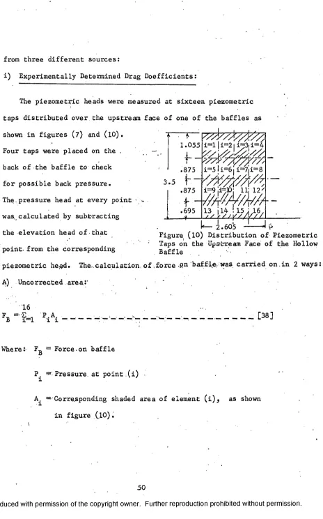
from three different sources:
i) Experimentally Determined Drag Doefficients:
The piezometric heads were measured at sixteen piexometric
taps distributed over the upstream face of one of the baffles as
shown in figures (7) and (10).
Four taps were placed on the .
back of the baffle to check
for possible back pressure.
The.pressure head at every point
was. calculated by subtracting
the elevation head of that
point, from the corresponding
1.055
f “
.875
i=l Ii~21 i=3i i=^f
i=5 I i=61 i=7ii=8
3.5
*“ '> i=9 I±=1D: 11: 12' .875
f
.695 -+
13 114 ! 15; 16/
// r / J Y~/ A/ / /
2.605
Figure (10) Distribution of Piezometric Taps on the Upstream Face of the Hollow Baffle .
piezometric he$d« The...calculation, of .force .pn baffle was carried on,in 2 ways
A) Uncorrected areas' ‘
16
FB ="?=1 P.A
Where:- F^ = Force-on baffle
P_^ ^'Pressure, at point.(i) •
A. = Corresponding shaded area of element (i)5 as shown
B) Corrected area:
16
F = 2 C P. A __________ ;__________________________ [39] i=l
Where: C = Correction factor to the areas. The correction i
factors were estimated from both the observed and assumed pressure
distribution along every row or column of piezometers.
Table (6), gives the selected values of (C^)
Table (6): Estimated values of correction factor (6^)
i C.
i i C. i C.i i. C.i
1 0.70 5 0.88 9 0.88 13 0.82
2 0.88 6 1.00 . 10 1.00 14 0.97
3 0.88 7 ' 1.00 11 1.00 15 0.97
4 0.70 8 : 0.88 12 0.88 16 0.82
Drag coefficients were calculated from equation [40].
2
Fg = CD x p x “ x A .__ ______ ____________
Where: F^ = force on the baffle in pounds
pF= density of water in slugs per cubic feet
v = initial mean velocity of flow in feet per second.
A = effective baffle area in square feet.
51
R eproduced with permission of the copyright owner. Further reproduction prohibited without permission.