HSU, CHIH-CHIEH. Efficient Evaluation of Highly Available Services: Fast Simulation and Testing. (Under the direction of Professor Michael Devetsikiotis).
Modern technologies have provided us with highly available services. Systems such as optical backbone networks, robust web servers, and reliable software can provide a service with unavailability probability lower than 10−6. Although rare, service unavailability can cause serious problems such as significant performance drop, or violation of Service Level Agreements (SLA). Moreover, providers of these services need to know the value of service unavailability probability so they can provide reasonable SLAs and corresponding Quality of Service (QoS). However, due to the extremely low values of the service unavailability probabilities, estimating them using traditional simulation or testing methods can require a vast amount of time to obtain a satisfactory confidence interval. As a result, efficient evaluation techniques are necessary.
by
Chih-Chieh Hsu
A dissertation submitted to the Graduate Faculty of North Carolina State University
in partial fulfillment of the requirements for the Degree of
Doctor of Philosophy
Computer Engineering
Raleigh, NC 2006
Approved By:
Dr. Do Young Eun Dr. Harry Perros
Dr. Yannis Viniotis Dr. Stephen Roberts
Biography
Acknowledgements
First and foremost, I would like to give my sincere appreciation to my advisor, Dr. Michael Devetsikiotis, for his guidance, patience, and support in every way during my PhD study. Dr. Devetsikiotis has brought me into the real world of academic research, and together we solved many interesting problems. This would undoubtedly be the most precious experience for my future career.
I would also like to express my gratitude to all the members in my advisory committee: Dr. Do Young Eun enriched my mathematical background, Dr. Steve Roberts solidified my basic and advanced simulation techniques, Dr. Harry Perros helped me verify my proposed methods against the numerical examples done by his team, and Dr. Yannis Viniotis helped to provide the testbed environment for me to apply my methods on. Without the help and valuable advises from them, my PhD research would be impossible to finish.
In addition, I would like to thank many people from IBM, especially Dr. Andy Rindos and Dr. Steve Woolet. During our cooperation, they shared their knowledge and expe-riences on practical software performance testing with me and enriched the scope of this dissertation.
Contents
List of Figures vii
List of Tables ix
1 Introduction 1
1.1 Highly Available Services . . . 2
1.1.1 Optical networks . . . 2
1.1.2 Robust network servers . . . 5
1.1.3 Reliable software . . . 6
1.2 Motivation . . . 8
1.3 Contributions of this Dissertation . . . 9
1.4 Outline . . . 10
2 Importance Sampling and Efficient Simulation 13 2.1 Basic idea of importance sampling . . . 13
2.2 Optimal biasing parameter and criteria for a good biasing . . . 15
2.2.1 Bounded relative error (BRE) . . . 15
2.2.2 Asymptotic efficient . . . 16
2.3 Overbiasing problem . . . 17
2.4 Dynamic IS simulation techniques . . . 18
2.4.1 Stochastic gradient techniques . . . 18
2.4.2 Stochastic optimization techniques . . . 19
2.5 Regeneration and A-cycle methods . . . 19
2.6 Conclusions . . . 21
3 Static and Adaptive Importance Sampling for Highly Available Services 22 3.1 Multi-service loss network modeling . . . 23
3.2 Existing IS methods for highly available services modeled as loss systems . 25 3.3 Static importance sampling using standard clock method (S-ISSC) . . . 26
3.3.1 Asymptotic efficient biasing for a single queue . . . 26
3.3.2 S-ISSC for multi-service loss networks . . . 26
3.4 Adaptive-ISSC (A-ISSC) . . . 31
3.5 Simulation model and results . . . 35
3.5.1 Simulation Models . . . 35
3.5.2 Simulation Results . . . 39
3.6 Conclusions . . . 46
4 Stochastically Optimized Importance Sampling Method 47 4.1 Performance Model for Optical Burst Switching Networks . . . 48
4.2 Simulated Annealing Optimized Importance Sampling Method . . . 50
4.2.1 Simulated Annealing . . . 51
4.2.2 Simulated Annealing Optimized IS . . . 51
4.3 Simulation model and results . . . 52
4.3.1 IS Model for OBS Network Simulation . . . 52
4.3.2 Simulation results and analysis . . . 54
4.4 Conclusions . . . 58
5 Performance Optimization Framework using Importance Sampling and the Response Surface Method 59 5.1 The Response Surface-Importance Sampling (RS-IS) Framework . . . 61
5.1.1 Response Surface Methodology . . . 61
5.1.2 The Response Surface-Importance Sampling Framework . . . 63
5.2 Simulation Model and Results . . . 65
5.2.1 Simulation Model . . . 65
5.2.2 Simulation Results . . . 66
5.3 Conclusions . . . 69
6 Summary of the Dissertation and Future Work 70 6.1 Summary of achievements . . . 70
6.2 Future work . . . 71
List of Figures
1.1 A seven-node optical network with all possible routes . . . 3
1.2 OBS network operation. . . 4
1.3 An example of robust network servers. . . 6
1.4 A simple example of Markov usage model. . . 7
1.5 Queueing model of a three server software. . . 7
1.6 The overview structure of this dissertation. . . 11
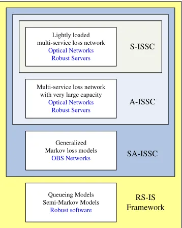
1.7 The relationship of models and evaluation methods in this dissertation. . . 11
2.1 Schematic illustration of the concept of IS. . . 14
2.2 “Backbone and rib” A-cycle Method. . . 21
3.1 Multi-service loss network. . . 23
3.2 Adaptive Importance Sampling. . . 32
3.3 Server breakdown probability caused by different kinds of error,λ=0.5. . . 39
3.4 Server breakdown probability caused by different kinds of error,λ=1. . . . 40
3.5 Relative error versus breakdown probability. . . 40
3.6 Blocking probabilities for routes using one link. . . 41
3.7 Blocking probabilities for routes using two links. . . 42
3.8 Blocking probabilities for routes using three links. . . 43
3.9 Blocking probabilities for routes using four to six links. . . 43
3.10 Relative error versus blocking probability. . . 44
3.11 Relative error versus blocking probability. . . 44
3.12 Efficiency versus blocking probability. . . 45
4.1 Decomposition of an OBS network into two sub systems. . . 49
4.2 OBS model used in this chapter. . . 50
4.3 State Evolution of SA-ISSC for a Single OBS Node. . . 56
4.4 State Evolution of SA-ISSC for a 5-Node OBS Network. . . 56
4.5 State Evolution of SA-ISSC for a 5-Node OBS Network. . . 56
4.6 Variance Evolution of SA-ISSC for a Single OBS Node. . . 57
4.7 Variance Evolution of SA-ISSC for a 5-Node OBS Network. . . 57
List of Tables
3.1 Error types in robust server simulation. . . 37
3.2 Error arrival rates in robust server simulation . . . 37
3.3 Call arrival rates in the simulated network. . . 38
3.4 Blocking probabilities and relative errors of Route 11, type 1. . . 41
3.5 Blocking probabilities and relative errors of Route 11, type 2. . . 42
Chapter 1
Introduction
Modern communication and computer systems are, or required to be, able to provide highly available services [55]. Examples of such systems include robust network servers, optical networks, reliable software, next generation wireless networks, and large computing grids. In such systems, high availability can be achieved either by low component failure rates (also in the sense that average fault recover time is much smaller than mean time between component failures), or by using a very large capacity or redundancy of resources. In systems that provide highly available services, unavailability due to complete system failure or lack of capacity can become rare events (in fact, this is routinely expected from such systems). In such cases, simulation or actual system testing based on standard Monte-Carlo methods may require an extremely long runtime, and usually incurs large relative errors. Importance Sampling (see [28]) has been known as a technique to improve the accuracy of estimates of stochastic events, which permits large speed-ups of estimation of extremely low failure probabilities. The system under study is simulated or emulated in a way that the “important” events occur more frequently by “biasing” the underlying probability distribution. In this dissertation, we explore and propose methods based on importance sampling for efficient simulation and testing of systems that provide highly available services.
will be illustrated in the last section.
1.1
Highly Available Services
Highly available services are usually encountered in systems which can provide ser-vices with very low unavailability probabilities, generally between 10−6 and 10−9, or even less. In this section, several illustrations of highly available services are introduced, includ-ing optical networks, robust servers, and reliable software. These illustrations of highly available services will be used as examples and for simulation experiments throughout this dissertation.
1.1.1 Optical networks
Traffic groomed optical networks
Modern optical techniques such as wavelength division multiplexing (WDM) have enabled the capability of carrying several Terabits per second by using multiple wavelengths, each of which can carry traffic streams at the order of Gigabits per second, in each fiber. However, in many cases, a traffic stream may only need a small fraction of the wavelength.
Traffic grooming (see [16]) technique allows the bandwidth of a wavelength to be divided
into smaller sub-rate capacities called sub-wavelength units. A customer can require one or more sub-wavelengths to a maximum of the bandwidth of a wavelength. The nodes that connect the links are add/drop multiplexors (ADMs). An ADM is the place where some of the traffic goes through while some other is dropped, which means that the traffic stream is directed to local traffic. Meanwhile, new traffic may be added from local sources, if there is sufficient capacity remaining.
either the very low call arrival rate, or to the very large capacity of the network.
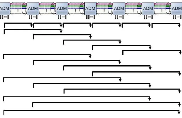
An example of a traffic groomed optical network can be found in [31]. For validation with numerical methods as in [59], consider a tandem network of multi-rate loss models with simultaneous resource possession. For example, Figure 1.1 illustrates an optical network with seven nodes and six links. In our simulation method, this topology can be extended to a more generalized mesh network without any difficulty.
Figure 1.1 also shows the possible routes in the network; that is, traffic of a call may arrive at any nodea, and leave at any other nodeb, wherebis to the right ofa. An incoming call may require one or more sub-wavelength units along its path, depending on the demand of that call. All of these sub-wavelength units are assigned to the call simultaneously at the time it is accepted. If a call is not accepted, it is considered blocked. When a call departs, all sub-wavelength units on all of the links along its route are simultaneously released.
Figure 1.1: A seven-node optical network with all possible routes
Optical burst switching networks
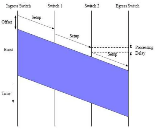
Figure 1.2: OBS network operation.
resources can be assigned and released dynamically as the traffic of the call travels, which is referred to as dynamic simultaneous resource possession. For example, in a relatively new optical switching scheme known as optical burst switching (OBS), multiple but not all resources can be reserved simultaneously [5].
In an OBS network, data packets are aggregated into various sizes of “bursts” at the edge routers, according to their destination. A burst could be a number of IP packets, an entire file, or frames from a video. Before a burst is transmitted, a control (or setup) signal, which contains the information of the burst such as burst length and expected arrival time, is sent along the same route to the destination as the burst itself to reserve the bandwidth (wavelength) along this route. A node in this route will reserve a wavelength for this burst at or after the control packet arrives, according to the reservation method used. After a time offset, the burst itself will be sent without having any acknowledgement from any of the nodes along the path. Figure 1.2 shows the basic operation of an OBS network.
when the burst fully passes one of the end nodes of that link.
If a burst is long enough, it is possible that the burst may occupy more than one links simultaneously. That is, it is possible that the burst may occupy a link between adjacent nodes A and B, and at the same time a link between adjacent nodes B and C. As the burst travels through the network, it will release the link that the whole burst has traversed and pick up a new link ahead. Therefore a burst may occupy two or more successive links, but these links change as the burst moves through the network, and thus the resources are dynamically simultaneously possessed.
If we assume that the network has large numbers of wavelengths, such an “one way” reservation mechanism would not sacrifice much performance drop due to burst losses while gain a lot from saving an one-way delay time from the destination to the source. OBS network architecture has been a hot topic for recent years, and there are many different implementation suggests for wavelength reservation and offset setting. However, a dropped burst usually contains mass amount of data and therefore burst dropping probability is considered an important index of service unavailability.
1.1.2 Robust network servers
Following the fast growth of demand for Internet services, network servers have been playing an increasingly important role. For a service provider, a server breakdown event may cause the service unavailable to requests, and possibly huge amounts of capital loss. As a result, redundancy is usually used to prevent servers from breaking down. Techniques such as server clusters [56] are introduced for risk diversification and load balancing. In the meanwhile, even for a single server in the cluster, techniques such as duplicated processors and network interfaces, disk arrays, and backup power sources have become standard in recent network servers. Together with physical redundancy, fast repair teams can also help making breakdown events rare.
Processors
Data Bus
Network Controller and Interfaces
Disk Array 1 Disk Array 2 Disk Array 3 Power
Modules
Power Line
Figure 1.3: An example of robust network servers.
failure of a power supply may also burn out several disks and processors. A single repair team or different teams can be assigned for a multiple component failure, and components failed together can be brought online again together when all failed parts are repaired, or one by one.
1.1.3 Reliable software
Performance evaluation of software could be performed by testing without assuming any model of the software. However, for modern software programs that are highly available and have very low request dropping rates, the use of direct testing could cost a lot of time while still not yielding satisfactory confidence intervals. The use of modeling has several benefits. First, efficient testing techniques could be used by the help of these models. Moreover, if real testing is expensive, simulation using the performance model can be used to assist real testing, so online capacity planning or performance evaluation would be more feasible.
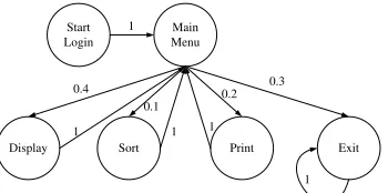
One of the most widely used performance models is the Markov usage model [24]. In this model, a Markov chain is constructed according to standard user behaviors, called
operational profiles, and the functions provided by the software. Figure 1.4 shows a Markov usage model of a software tool for displaying, sorting and printing items.
Start Login
Exit Print
Sort Display
Main Menu 1
1 1 1
1 0.1
0.4 0.2 0.3
Figure 1.4: A simple example of Markov usage model.
ȝ1 ȝ2
Requests Arrival
Events Arrival
User Interface Server
Event Server
Database Server
Ȝ1
ȝ3
Ȝ2
Figure 1.5: Queueing model of a three server software.
software under evaluation. Performance simulation using various techniques can then be applied. However, at the time of evaluation one may not be able to know the detailed behavior of the users. Moreover, the model can be complicated to build, especially when the software is distributed among several physical machines, which is becoming common in modern server software.
1.2
Motivation
For highly available services, including those introduced in the previous section, the service unavailability probability is an important indicator of quality. Due to the rarity of unavailability events, traditional simulation / testing methods are usually not suitable for estimating their probability. Numerical approximation methods have been developed to solve for these indicators. For example, [59] and [6] focus on solving the new call blocking probabilities of optical networks. We would like to develop ways that are both easy to use and accurate in estimating such quality of service indicators, based on Monte Carlo methods and Importance Sampling.
Multi service loss networks are widely used in modeling systems that provide highly available services. For example, [49, 40, 37], and [38] used multi service loss networks to describe these systems. One advantage of such a model is that the likelihood function of importance sampling is easier to calculate, provided that the arrival and service distributions are not too complicated. As a result, we would like to first consider using multi-service loss models in our development of efficient simulation methods.
There are many criteria and goals for the design of importance sampling methods that simulate rare events. Most of these criteria focus on the asymptotic performance of importance sampling methods as the value to be estimated approaches zero. We would like to explore such metrics of performances of our method if possible. On the other hand, since the value to be estimated does not usually approach zero asymptotically, there may exist methods that are better for practical values. In this dissertation we also put efforts in developing methods with these characteristics, especially for those models that are more complex.
1.3
Contributions of this Dissertation
The main contributions of this dissertation can be listed as the following:
• Analytically proven IS method for multiple-class, heterogeneous-demand
loss systems
Many highly available services of interest can be modeled as multi-service loss net-works, which will be introduced in Chapter 3. For such models, several methods have been proposed to use Importance Sampling in estimating the blocking probabilities, e.g., [49] and [40] focused on the estimation of the most likely blocking link; and Las-sila et al. [37, 38] provided methods for the cases in which more than one link may have contribution to the blocking probability. These methods are based on a product form solution and may need to calculate the very large table of transition probabilities or rates before the simulation begins.
In [58], the authors proposed Importance Sampling applied to the Standard Clock method (ISSC) and showed that in the single-class, homogeneous demand case, when the arrival rates approach zero, ISSC has bounded relative error in the estimation. In this dissertation, we extend this result to amulti-class service model with hetero-geneous demands, and therefore allow different types of simultaneous failures in the system. We prove this extended Static ISSC method still has the bounded relative error property and, thus, can be applied to efficiently evaluate models that are more complex.
• Better heuristic near-optimum IS method
For the case in which the failure rates do not tend to zero, we propose usingAdaptive ISSC, that tunes the probability distribution toward the most possible target in each step. Using A-ISSC, we avoid calculating excessively large tables in advance and we can extend existing methods for single link failure to more general cases, while still having very low relative estimation errors in the simulation. We also compare our proposed method with existing IS methods on different simulation cases, and prove empirically that our method can produce accurate estimation, and is more efficient than other methods that have already been published.
There are cases in which the importance sampling biasing can be done, but due to the complicated system model or incomplete knowledge of the system, minimizing the estimation variance becomes very hard, if not impossible. For such cases, we propose minimizing the variance directly using a stochastic optimization method, namely simulated annealing [1]. The proposed Simulated Annealing optimized ISSC (SA-ISSC) can be applied to almost any models, as well as the likelyhood of the IS method can be calculated correctly. Moreover, SA-ISSC is very easy to apply and can produce favorable results.
• Automatic metamodeling and optimization framework with efficient trace
reuse
It is not uncommon that one may want to know the performance of a system for more than single parameter configurations. One could even want to find an optimal configuration of the system that optimizes the performance or related indices. To deal with this, metamodeling methods, such as Response Surface Methodology [9], have been proposed for a long time. On the other hand, it is rarely seen that efficient evaluation techniques being used together with such metamodeling methods. In this dissertation, we propose a combined Response Surface-Importance Sampling (RS-IS) framework that automatically models and even optimizes the performance index of interest. Moreover, due to the nature of local sampling in the response surface method, we also propose a novel IS trace reuse strategy that saves even more evaluation time, while still produces very accurate solutions.
1.4
Outline
Figure 1.6 shows the basic structure of this thesis. The left-hand side of the figure shows some examples of highly available services we will evaluate, and the models used to describe these services. The right-hand side, on the other hand, shows the importance sampling-based methods we develop in this thesis to efficiently evaluate these services de-scribed by the models.
Traffic Groomed Optical Networks
Highly Available Services
Optical Burst Switched Networks
Robust Network Servers
Reliable Software
Multi Service Loss Networks
Markovian Loss Networks
Importance Sampling
Static IS Methods
Adaptive IS Methods
Dynamic IS Methods
Metamodeling Ω IS Frameworks Evaluate By
Simulation / Testing
Systemwide Evaluation / Optimization Queueing Networks
Figure 1.6: The overview structure of this dissertation.
Lightly loaded multi-service loss network
Optical Networks Robust Servers
Multi-service loss network with very large capacity
Optical Networks Robust Servers
Generalized Markov loss models
OBS Networks
Queueing Models Semi-Markov Models
Robust software
S-ISSC
A-ISSC
SA-ISSC
RS-IS Framework
the range covered by each rectangle implies the models that such a method can be applied to. Throughout the paper it will be shown that although a method covering more services and models could be applied on all of them, for the models also covered by another smaller rectangle, this more general method is usually not as efficient as the methods denoted by smaller rectangles, for they are generally been optimized according to the model.
Chapter 2
Importance Sampling and Efficient
Simulation
2.1
Basic idea of importance sampling
Importance Sampling (IS) is a Monte Carlo (MC) estimation technique which aims to reduce the variance or other cost function of a given simulation estimator. Figure 2.1 illustrates the concept of importance sampling. Assume we want to measure the two-dimensional area of region B by simulation. Traditional Monte-Carlo (MC) simulation generates points in A from a uniform distribution, and the estimation of region B would be
b
B = NB
N , where NB is the number of “hits” within area B, and N is the total number of
A=1 B C A=1 B C D
Figure 2.1: Schematic illustration of the concept of IS.
Consider a case in which we want to estimate the probabilityP(X∈B) for a random variable X with probability density function (pdf) f(·). Traditional Monte-Carlo simula-tion method generates samples of X and counts the number in B, that is, by estimating E[1{X∈B}],where1{} is the indicator function, and E£1{x∈B}¤=P(x∈B). If P(X ∈B) is very small, it would require a large number of samples for the estimator to be accurate. This is because the relative error, which is defined to be the standard deviation divided by the mean,
√
P(X∈B)(1−P(X∈B))
√
nP(X∈B) =
q
(1−P(X∈B))
nP(X∈B) goes to infinity as P(X ∈ B) → 0.Using IS, we generate samples with abiased pdff∗(·) withP∗(X ∈B)> P(X∈B).If each time we observe an x within B, we increment our count by ff∗((xx)) instead of 1, then, effectively,
we are constructing a new “weighted” random variable, the expectation of which is also equal toP(X ∈B):
Z
x∈B
f(x)
f∗(x)f∗(x)dx=
Z
x∈B
f(x)dx=P(X∈B).
The function L(x) , f(x)
f∗(x) is called the Radon-Nikodym derivative, or the likelihood ratio.
For a Markovian-type system, if we have a sample pathxwithM steps, the Radon-Nikodym derivative would be product of the Radon-Nikodym derivative in each step alongx, that is,
L(x) = f(x)
f∗(x) =
MY−1
k=0
f(xk, xk+1)
f∗(xk,xk+1) (2.1) where f(xk, xk+1) and f∗(xk, xk+1) denote the original and biased transition probability from state xk toxk+1,wherexk is the system state at the kth step.
whenever f(x) > 0, then we must also have f∗(x) > 0), the IS estimator is statistically unbiased. However, deciding how to choose an appropriate L(x) so that the simulation is most efficient and results in smallest variance is far from trivial, depending on the system of application.
2.2
Optimal biasing parameter and criteria for a good biasing
Consider the following change of measure.
f∗(x) =
f(x)
P(X∈B), x∈B
0, otherwise .
In other words, this new distribution is simply the original one conditioned on the oc-curing of the rare event we are interested in estimating. By doing this, we haveL(x)1{x∈B}=
P(X ∈B) for anyx obtained in the new sampling distribution, and, thus, the variance will be 0, and only one sample gives usP(X ∈B) exactly. Therefore,f∗(x) is the optimal change of measure. Actually, this optimalf(x) can be easily derived directly by using Jensen’s in-equality [54]. However, sincef∗(x) explicitly depends onP(X∈B), the unknown quantity that we are trying to estimate, this change of measure is can not be practically used. If
P(X ∈ B) were known, there would be no need to run the simulation experiment at all. Nevertheless, in the development of efficient importance sampling methods, this “Optimal Biasing” can be used as a guideline in choosingf∗(x). This leads to the following principles for a good f∗(x):
• Choose f∗(x) so that we “hit” the events of interest A as often as possible.
• Choose f∗(x) so that the more likely or higher probability regions ofB will be “hit” more often during the simulation than the lower probability or less likely regions of
B. That is, we want to find af∗(x) that the “relative probabilities” of elements inside setB are kept the most.
2.2.1 Bounded relative error (BRE)
an IS estimator is to determine if it has bounded relative error (BRE), which checks if the relative error, defined as the standard deviation of the estimator divided by the estimator itself, can be bounded as the probability to be estimated approaches zero (see [52] and [28]). The definition is as follows:
Definition 1 Assume we would like to estimate the probability Pε(X ∈B) of a rare event, wherePε(X ∈B)→0asε→0.An unbiased IS estimator forPε(X ∈B)=E[L(X)1{X∈B}],
has bounded relative error (BRE) under f∗(x) if there are constants δ < ∞, ǫ0 > 0 such
that
sup
ǫ≤ǫ0
q
Var∗[L(X)1{X∈B}]
Pε(X ∈B) ≤ δ.
The following lemma is a direct consequence of the above definition [11].
Lemma 2 If there are constantsα, βandγsuch thatPε(X ∈B)≥αεγandL(X)1{X∈B}≤
βεγ a.s., then the IS estimator for Pε(X∈B) has BRE.
We can see that the relative error is actually proportional to the relative half-width of the confidence interval in the simulation. As a result, having an estimator that has BRE is indeed very preferable, since one always needs only a fixed number of iterations to obtain a target relative confidence interval, no matter how rare the corresponding event is.
2.2.2 Asymptotic efficient
Generally, it is not easy to find an IS estimator that has bounded relative error. Another widely used criteria for a good IS estimator isasymptotical efficiency. The idea of asymptotically efficient comes from large deviation theory.
As stated in earlier sections,
N V ar(P(\X∈B))n= h
En12{X∈B}L(X)o−P(X ∈B)2i
n ,¡FB−P(X∈B)2¢
wheren is a rarity index. That is,P(X∈B) goes to 0 asn goes to infinity. From large deviation theory, we have (under some assumptions)
lim
n→∞
1
nlog(P(X ∈B))n=−I
lim
n→∞
1
nlog(P(X ∈B))n=−R
Since variance is always greater or equal to zero, we have R≤2I. IfR = 2I, this IS method is said to beAsymptotic Efficient.
In other words, asymptotic efficient means the relative error will not grow exponentially as the value to be estimated approaches zero.
2.3
Overbiasing problem
When applying importance sampling, choosing of the biasing distributions must be done with care. Carelessly chosen biasing methods may not result in a satisfactory variance reduction. A bad IS design can even enlarge the estimation variance! This is sometimes called a “backfire” in variance reduction methods. In importance sampling, such a problem can be referred to as “overbiasing”. Overbiasing is dangerous, since it not only potentially increase the estimating variance, it can even cause error if the simulation is carelessly performed.
For example, consider the following examples. Let A={x1, x2},is the area we would like to estimate, whereP(x1) = 10−5,andP(x2) = 2·10−5. P(A) = 3·10−5.
The “optimal” biasing that will give us zero variance is
P∗(x1) = 1 3, P
∗(x2) = 2 3, in which both likelihood ratios is equal to 3·10−5. However, if we use the following biasing,
P∗(x1) = 0.9999, P∗(x2) = 0.0001 we have
Although this estimator is still statistically unbiased, in practical we will getx1 most of the time. If the simulation is not performed long enough, one may have an estimation that P(A) = 10−5 with a very low variance, while in fact this estimation is not even near the actual value.
2.4
Dynamic IS simulation techniques
To use importance sampling in rare event simulations, it is good to have an impor-tance sampling distribution with bounded relative error or asymptotical efficient property. However, to have such an distribution, it is usually required to have a good understanding of the system, or the large deviation behavior of the rare event of interest. Therefore, there are many research which aims directly on minimization of the variance of the estimator (for example,[34, 17, 14]). Such techniques are called dynamic IS techniques, or sometimes, adaptive IS techniques.
2.4.1 Stochastic gradient techniques
Let fθ(x) denote the family of candidate distributions to be used in importance
sam-pling. To minimize the variance of importance sampling simulation for PA = P(X ∈ A)
under the original pdf f(x) can be formulated as
min
θ V arfθ[1{X∈A}Lθ(X)]
where Lθ(x) = ffθ((xx)).Since
V arfθ[1{X∈A}Lθ(X)] = Efθ[1{X∈A}Lθ(X)
2]−E
fθ[1{X∈A}Lθ(X)]
2 = Efθ[1{X∈A}Lθ(X)
2]
−PA2,
the variance-minimization problem is equivalent to
min
θ Efθ[1{X∈A}Lθ(X)
2],
R-M algorithm uses the following recursion to obtain the optimal θ:
θn+1= ΠΘ(θn− a
n+ 1▽ch(θn))
,where ΠΘ is the projection operator onto Θ, h(·) is the objective function (that is, Efθ[1{X∈A}Lθ(X)
2]) and ▽ch(θ
n) is an estimate of ▽h at θn. To get ▽ch(θn), several
techniques such as infinitesimal perturbation analysis [20], likelihood ratio methods [22], Conditional Monte Carlo [19], and the “push-out” approach [50] can be applied. K-W algorithm also uses the same recursion formula, but use different method to estimate▽h(θn).
Using importance sampling for accelerating simulation by finding an approximate min-imizer of variance of the estimator has been applied in various applications, especially in queueing and reliability models; see, e.g. [2, 14, 13].
2.4.2 Stochastic optimization techniques
Simulated annealing (SA) [36] is a widely used optimization method that can avoid being trapped in local optimum. In simulated annealing, in addition to the moves that decrease the cost function, a move which causes an increasing cost of ∆C will be taken with some probability related to a parameterc, which is called thetemperature. From time to time, the temperature is lowered from Tmax to Tmin, thus lowering the probability of accepting uphill moves and forcing the system into a global minimum.
Simulated annealing can be used to minimize IS variance. In [14], a variation of SA, Mean field annealing (MFA) [8], is used to obtain minimum variance of importance sampling simulation for a single queue. The MFA algorithm keeps the ability of SA to avoid local minima, and converges faster than SA, but is not guaranteed to converge.
2.5
Regeneration and A-cycle methods
We are often interested in steady-state properties in simulations of stochastic systems. For example, in queueing models, one might be interested inP(Q > x) whereQis the steady state queue size distribution. If the system is regenerative, we can use the “regenerative
method” to estimate steady state QoS parameters. In a regenerative system, there exists
distribution, as if the process were started at the state. The system evolution between two consecutive visits of this state is called aregenerative cycle. LetTi denote the length of the ith regenerative cycle. If E[Ti]<∞, the system has steady state distribution X. Let h(·)
be a function on the state space and define Yi = Rithcycleh(Xt)dt, where Xt denotes the
sample in timet. Then
E[h(X)] = E[Yi]
E[Ti] .
For a highly available service, usually a non-zero Yi is a rare event. Therefore,
im-portance sampling can be applied to estimate the numerator. Imim-portance sampling is used until a non-zero value of Yi, occurs, and then it is “turned off”, and the system will then
return to the regenerative state naturally. The denominator is simply the expected cycle time, so it is not necessary to use importance sampling to estimate the denominator. If under importance sampling, the system is still regenerative, importance sampling may be left “on” when the rare event occurs. However, in many cases the importance sampling distribution is chosen so that the system will not regenerate (even unstable). In such cases, importance sampling should be turned off in order to permit regeneration. In [14], the authors even use another set of importance sampling distribution to force the regeneration to happen.
In some applications, the model may not be regenerative, but a similar formula still exists. For a quasi-regenerative set Awhich will be visited infinitely often, define A-cycles to begin whenever the process entersA. Then
E[h(X)] = E[Yi(A)]
E[Ti(A)] .
whereYi= R
ithAcycleh(Xt)dtandTi(A) is the length ofithA-cycle. Similarly,
impor-tance sampling can be used to estimate the numerator, while standard simulation can be used to estimate the denominator. Such method is usually called A-cycle method.
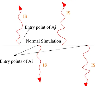
Figure 2.2: “Backbone and rib” A-cycle Method.
the entry points for the different IS simulations. For confidence interval in this method, Jackknife technique may be used.
2.6
Conclusions
Chapter 3
Static and Adaptive Importance
Sampling for Highly Available
Services
Most of the importance sampling techniques mentioned in previous chapter focus on estimating bit error rate or overflow probability in a queue. In other words, there is only one objective that is of interest. For example, if we are interested in the buffer overflow probability of one certain queue in a feed forward queueing network, we will try to change the measure so that buffer overflow in that queue will not be a rare event. This procedure may not be true in real-world highly available services, where a rare event we are interested in may happen in more than one place. For example, an highly available optical network will be well designed so that there will not likely to be a single bottleneck for a call that uses multiple links. Instead, the call blocking, which is a rare event, could happen because any of the links it uses does not have enough wavelengths available.
Resource 1 Resource 2 Resource 3 Resource 4 Resource 5 Resource 6
Figure 3.1: Multi-service loss network.
a brief survey of existing importance sampling methods for highly available services will be introduced. Then, we propose two importance sampling methods that can be used to estimate the blocking probability of the multi-service loss model. The generalized Static Importance Sampling using Standard Clock (S-ISSC) method is first introduced and proven to have BRE property, even under a multi-class service model with heterogeneous demands. Then the Adaptive Importance Sampling using Standard Clock (A-ISSC) method, which is based on the approximation of the “optimal biasing”, is introduced.
3.1
Multi-service loss network modeling
Among the services introduced in the first chapter, the traffic groomed optical network, the robust server, and many other similar services can be modeled as multi-service loss networks. This allows us to unify the notation and the features of the importance sampling technique that we will present in the following sections.
Figure 3.1 shows a loss network with sixtypes of resources, each with possibly different capacities, and with several possible call demands, shown as arrowed lines. A call can require two or more types of resources that are not physically connected. An arriving call may require different numbers of units from different types of resources, depending on the
in an optical network, or to an event of the network server being in the breakdown mode. In both cases, this means the service is unavailable.
Assume there are R ∈ N types of calls and L ∈ N types of resources, each type
r, r = 1,2, . . . , R call has a demand of dr,l ∈ Z+ units of type l, l = 1,2, . . . , L resource
when it arrives. An arriving call of type r will be accepted only when every resource type
lin thedemand set, Dr ,{l:dr,l>0},that the call needs has at leastdr,l units available.
If a call is not accepted as the time it arrives, it will be blocked. A blocked call will simply be discarded, and the system state will not change.
In general, we assume that resource type l in the loss network has a capacity of Wl
∈ N units. Type r calls arrive at rate λr ∈ R, and all calls have a mean call duration of
1
µ, µ ∈R. In this dissertation, we assume that both inter-arrival times and call durations
are exponentially distributed. This could be relaxed in the future. As noted, a call of type
r will be accepted only if there are at leastdr,l units of resource type l available, ∀l∈Dr.
For an optical network, traffic demands for a type of call are usually the same for each type of resource (optical link), that is, dr,l are equal for all l ∈ Dr. This is referred to as
homogeneous demand here in this dissertation. Moreover, for optical networks Dr always
forms a “route” that is physically connected. Therefore, we may also categorize the calls according to the route and the class of a call.
In practice, the call blocking probability for each type of call is important in the case of optical networks, since a large unavailability probability can mean violation of the service contract (or “SLA”, server level agreement) for a certain type of call. For robust servers, knowing the probability of a certain failure type being the last failure to cause system breakdown may also be important, since this relates to the possible cost of recovering from the breakdown. Moreover, if we know the probability of breakdown seen by every type of error, the overall service unavailability probability will be easy to calculate.
3.2
Existing IS methods for highly available services modeled
as loss systems
Methods for accelerating the simulation of packet-based networks of queues have been known for a while (see [28, 53, 17] and references therein). For reliable systems that can be modeled as Markov chains, there have been several publications regarding fast performance evaluation of highly . See [44] for a survey of such methods. The general idea of these methods is to change the “weights” of every possible path to failure state. Several of them are proven to have the BRE property. However, as mentioned in the introduction, when the system grows large, the number of states of the Markov chain can be very large, and similarly when multiple component failures are allowed. Since this complicates the transition of the Markov chain, such methods may become inefficient. By using loss networks, one has only to consider ways to “fill” the resources, rather than to account for every path to failure states, and therefore loss networks could offer a preferable model for such cases.
Consider a multi-service loss network as stated in section 2.3. In the demand set of a type of call, if call blocking events happen for a certain type of resource, say l′, far more frequently than in all of the other types of resources, we can estimate the call blocking probability by changing the distribution under importance sampling (also calledbiasing the distribution) towards overwhelming resource typel′.This can be called asingle target system
3.3
Static importance sampling using standard clock method
(S-ISSC)
In this section, we introduce an importance sampling simulation technique called static IS using standard clock (ISSC). The original static ISSC method is introduced in [58] to estimate the call blocking probability in a cellular telephone network with dynamic channel assignment. In [4], a dynamic method is used to estimate the call blocking probability in wavelength continuous WDM networks with single wavelength demand.
3.3.1 Asymptotic efficient biasing for a single queue
The idea of static ISSC comes from the asymptotically efficient exponential IS biasing methods in single server queues. In an M/M/1 queue, this method is simply exchange of arrival rate and service rates. As a result, in static ISSC we would like to extend this method to exchange of arrival and service rates of calls that have relationship with the call that we are interested in.
3.3.2 S-ISSC for multi-service loss networks
In this section, we generalize the formulation of the static ISSC method from [58] to include multi-class systems and prove that the method still exhibits a BRE in this more general setting, allowing us to apply the method to the large class of loss systems outlined in the previous sections.
Using a similar but generalized notation as in [4], we defineSl as the union of all call
types that use the resource type l, and Cr, which is called cluster r, to be the union of all
call types that use any resource call type r also uses. That is,
Sl={call type i:l∈Di}, Cr ={call type i:Dr∩Di 6=∅}.
If we define an event to be either an arrival or a departure of a call, we can use Nr
P
r(Nr·dr,l) ≤ Wl, ∀l = 1, . . . , L}, where, as defined in Section 2, dr,l represents units of
resource typela typercall demands, and Wl stands for the capacity of resource typel. In
other words, a system state N is said to be valid if every type of resource does not exceed its capacity. Finally, for type r calls, the system reaches a blocking state if any resource type l has less than dr,l units unused. Since a blocked call will be discarded and will not
change the system state, a system starting from any valid state will remain in the set of valid states.
Assume inter-arrival times and service times are exponentially distributed. Under
theStandard Clock simulation approach [57], consider applying Importance Sampling. We
would like to change the arrival rates and service rates of some calls, so the blocking prob-ability for the call typer, in which we are interested, becomes a non-rare event. Theevent rate for the system at state N before applying IS is
ΛN = R X
i=1
λi+µ R X
i=1
Ni.
Consider the change of measure that swaps the aggregate arrival rate of calls in cluster
r, λ= P
i∈Cr
λi, with service rate µ [58]. That is, the new inter-arrival times of call type i, i ∈ Cr, are exponentially distributed with rate λ∗i = λλiµ. As a result, the total arrival
rate of calls in Cr becomes λ∗ = µ. Service times for these calls are now exponentially
distributed with rate µ∗ = λ. Inter-arrival and service times outside the cluster have the original exponential distributions. The new event rate at stateN becomes
Λ∗N =µ+X
i /∈Cr
λi+λ X
i∈Cr
Ni
+µX
i /∈Cr
Ni.
Now consider a system with IS “turning ON” at event “0”, which is the event immedi-ately before the “first event” in the following discussion. UsingN(j) ={N1(j), N2(j), . . . , NR(j)}
to denote the system state just after the jth event, the corresponding Radon-Nikodym derivative at themth event is
L(m) =
mY−1
j=0
ΛN(j)e−ΛN(j)Tj+1
Λ∗
N(j)e
−Λ∗ N(j)Tj+1
×
mY−1
j=0
Λ∗N(j)
where Tj is the time between the (j−1)th event and the jth event, and
H(j) =
λ µ, j
th event = arrival of call typei, i∈C
r µ
λ, j
th event = departure of call typei, i∈C
r
1, otherwise.
Letabe the total number of arrivals to clusterr inm events, anddbe the total number of departures to clusterr inm events. We can rewrite L(m) as
L(m) =e− mP−1
j=0
(ΛN(j)−Λ∗N(j))Tj+1µλ
µ
¶a³ µ λ
´d .
Moreover,
Λ∗N(j)−ΛN(j)=µ+
X
i /∈Cr
λi+λ X
i∈Cr
Ni(j)
+µX
i /∈Cr
Ni(j)− Ã R
X
i=1
λi+ R X
i=1
Ni(j)µ !
=−(µ−λ)(X
i∈Cr
Ni(j)−1).
Therefore,
L(m) =e−
(µ−λ)
"
mP−1
j=0
( P
i∈Cr
Ni(j)−1)Tj+1
# µ
λ µ
¶a−d
. (3.1)
Finally, assuming that Br is the event that the system is in any blocking state for call
type r in steady state, and M is the random number of events just after the system first enters a blocking state while using IS, then we have
P(Br) =E[1(Br)]
=E∗[L(M)·1(Br)]
whereE∗[·] means the expectation with respect to the IS biasing distributions.
For the simulation, we use the quasi-regenerative (orA-cycle) technique introduced in the precious chapter. If an A-cycle is started from the stationary distribution conditioned on the process just entering A, the blocking probability can be expressed as
P(Br) = E[TB] E[TA]
= E[TB|AB]P(AB)
where TA, TB and AB are the A-cycle length, time spent in blocking states of call type r
in an A-cycle, and the event that an A-cycle contains any blocking state or call type r, respectively.
These quantities (A, TA, TB,andAB) should all be related tor,the type of the call we
are interested in, but here we omit therfor simplicity. We can estimateP(AB) by “turning
ON” IS when the system state reaches A from A′, and until it reaches a blocking state. Then we “turn off” IS and perform ordinary simulation from this point until the system leaves the set A, and E[TB|AB] can be estimated. Moreover, since it is not rare for the
system to be in anA cycle (A-cycles typically have a significant, non-infinitesimal length), we can simply use ordinary simulation to estimate E[TA] without IS.
As mentioned above, an A-cycle should be started from the stationary distribution conditioned on the process just enteringA.However, IS changes the underlying distribution and therefore the simulation run after an ISA-cycle cannot be re-used for anotherA-cycle. A “splitting” technique [28] can be used, in which an ordinary simulation is run in parallel to the IS to provide entry-points for IS A-cycles. Each IS simulation starts at one of these entry points with IS “turned on”, then “turns off” IS when the system reaches a blocking state, and finally ends as the system leaves setA. Actually this ordinary simulation can be run in advance, and can also be used to estimate E[TA]. For different call types that have
different definitions of the set A, the same ordinary simulation can be re-used for all the entry points of theseA-cycles. In this chapter, we define set A for call typer to be the set of all states in which the number of calls in cluster Cr is greater than zero.
3.3.3 BRE property of S-ISSC
In the following, we extend our result from [31], which follows a generalized procedure as in [58], to prove that under lightly loaded situation, the static ISSC method will have Bounded Relative Error (BRE).
Theorem 3 Assume there are constants ǫ, ϕi ∈ R such that λi = ϕiǫ, ∀i,and µ > λ = P
i∈Cr
Proof Without loss of generality, assume that we are interested in estimatingP(AB)
of call type r. We would like to prove the BRE using Lemma 2. Consider a blocking state of typer calls that need the least number of active calls in clusterr. For each resource type
l ∈Dr,the demand set of call r, let
bl1=
Wl
max
i di,l
, r1 ,arg max
i di,l
bl2 =
Wl−bl1·dr1,l
max
i,i6=r1
di,l
, r2 ,arg max
i,i6=r1
di,l
.. . until minis.t. X
i
bli·dri,l ≥Wl−dr,l
bl= X
i bli,
and
b= min
l∈Sr
bl.
In other words, we exhaust resource type l by first using bl1 call arrivals of the type which needs the most units of resource type l, until no more such calls can be accepted.
Then the second-most demanding type of calls are used to exhaust the resource type, and repeated until reaching a blocking state for typer calls.Minimizing overl∈Sr,we obtain
the minimal number of active calls needed for a blocking state for type r calls.
From the definition above, we know that if the system reaches a blocking state for type r calls just after themth event happens, there are at leastb active calls within cluster
r. Moreover, from the definition of A, the active calls within cluster r will be at least one. Since µ > λ and P
i∈Cr
Ni(j)≥1 in setA, we have
(µ−λ)
mX−1
j=0
à X
i∈Cr
Ni(j)−1 !
Tj+1
≥0.
Furthermore, since a−d≥band µ > λ,we have
µ
λ µ
From (3.1), we obtain
L(m)1{AB} ≤
µ λ µ ¶b =αǫγ, where α= Ã X
i∈Cr
ϕi/µ !b
,
and
γ =b.
Next, we need to show that P(AB)≥βǫγ =βǫb.Consider a sample path to reach the
state of active calls mentioned above, by arrival events only. This will bring the system into a blocking state of call type r, and the probability of this sample path is a lower bound of
P(AB).
Usingλ(j) to denote the arrival rate of the call type which arrives as thejthevent, we
have
P(AB)≥
bY−1
j=0
µ
λ(j+ 1) ΛN(j)
≥
µ
minjλ(j+ 1)
maxjΛN(j)
¶b
≥
µ
minjϕjǫ bµ+Piλi
¶b
=βǫb
whereβ =³ minjϕj
bµ+Piλi
´b .
From all of the above and Lemma 3.2, it follows that static ISSC has bounded relative error (BRE).
3.4
Adaptive-ISSC (A-ISSC)
Blocking at Resource 1
Current State
Call Type 1
C al l T y p e 2 B lo ck in g a t R es o u rc e 4 Sample Target Resource
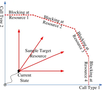
Figure 3.2: Adaptive Importance Sampling.
together with ISSC and theA-cycle method described in the previous section, we introduce Adaptive ISSC (A-ISSC) in this section.
Assume that we want to estimate the blocking probability in a multi-target system, where the blocking could happen due to the lack of more than one type of resource. The idea of adaptive biasing is introduced in [26] for multi-class, homogeneous demand networks, where an arriving call requires the same number of units among the resource types in its demand set. In [27], this method is applied to non-homogeneous demands, and calls with different priorities.
In this section, we use the basic idea from [27] but introduce a simpler resource sam-pling approach and a different biasing method, and apply them to the general loss network model for highly available services, with multiple classes and non-homogeneous demands.
Our method works as follows: First pick a type of resource from a probability distribu-tion that reflects the relativeimportance of each resource type that could lead to a blocking state. Then the system is biased using importance sampling, as if the sampled resource type is the only target. After anevent, another sampling of resource types is done, and the IS biasing distribution is changed again to bias the system toward the newly selected type of resource. These steps are repeated until the system reaches a blocking state for the call type in which we are interested. The idea is shown in Figure 3.2, where a simplified model of four types of resources and two types of calls are shown.
state. It is known (see [28]) that if we want to use IS to estimate the probability that a random variableX, with pdf f(x),is in a setB, theoptimal IS distribution f∗(x) is:
f∗(x) =
f(x)
R
x∈Bf(x)dx
x∈B
0 otherwise.
That is, sample only the elements inBand also preserve the relative probabilities of elements in B. It is obvious that this distribution requires the understanding of the probability we want to estimate and, thus, is not feasible. However, biasing the probability distribution so that the relative probabilities of elements in the importance set can be preserved does help one prevent over-biasing problems and reduce the estimator variance [28]. In a dynamic case like our loss network, it is usual that even the relative probabilities cannot be easily estimated. As a result, we would likefbN(l) to be a distribution that approximately preserves
the relative probabilities the system will be in the blocking states of call typer, due to the lack of resource type l, starting from state N. We can estimatefbN(l) by calculating how
easily the blocking state of resource type lcan be achieved from the current stateN.
In [25], methods are suggested for calculating fbN(l), which are based on a weight for
eachl that is a product ofcontribution and likelihood. In [26], a more complex algorithm is suggested. In [12], the author suggest using cross entropy as the guide to do the sampling. Here we propose using the probability of theshortest path from stateN to a blocking state that is due to the lack of resource typel as the weight of type l. fbN(l) is a probability
distribution that is proportional to the weight of resource type l. Similar ideas using IS based on shortest paths can also be found in simulating reliability systems (see [3] and [10]) To calculate the weight, consider the most likely path to reach a blocking state for call type r from current state N. For a system with arrival and service rates independent of system states, such as the model we use in this chapter, the shortest path would correspond to successive arrivals of call of traffic typei, whosedi,lλµi is the largest among all call types
that use class l, until the system reaches the blocking state of call type r. Since di,lλµi is
independent of system states, this can be calculated in advance; and in each step, we only need to calculate kDrk weights, where kDrk is the number of resource types in Dr, one
for each type of resource used by the call type in which we are interested. Our simulation result shows that using this method, fbN(l) can be calculated efficiently (as in the following
algorithm), while the estimation of blocking probability is still accurate.
the call duration rates are dependent on the system state. For such cases, we have to consider all possible sample paths, which may require an excessive amount of computing time. One possibility is to choose the largest di,lλµii((NN)) for each step and use this resulting
path as the shortest path, whereλi(N) andµi(N) are arrival and service rates for call type i in system state N. This method requires O(kDrk ·N(c)) computations, where N(c) is
the mean value of the number of call types that use resource typel over thekDrk resource
types that the call type of interest, r, is using.
After the target resource type bl is decided, we can then bias the system toward that type of resource. Exponential biasing, which is often suggested in single target systems, can be used. For exponentially distributed inter-arrival and service times, a interchange of the aggregate arrival rate of the call types that use resource type bl with the aggregate service rate of the active calls that use resource typebl, may also be used (a biasing which is asymptotically optimal in single-class systems).
In a system with very large capacity, a modification of the dynamic method provided in [58] could be applied for biasing the system toward resource typebl. Let the number of active calls that uses resource typeblbeNe(bl), and consider the following change of measure:
λ∗(Ne(bl)) =bλ+Ne(bl)(µ−µ∗(Ne(bl)))
µ∗(Ne(bl) + 1) = bλµ
λ∗(Ne(bl)), wherebλ=Pi∈S
lλ,andµ
∗(0) = 0.This method is proved to be optimal in a single resource type, single call type case, and to have the BRE property in a single target case with multiple classes of call demands.
Our Adaptive ISSC algorithm to estimate the blocking probability for call type r, starting from an entry point of an A-cycle, which has the same definition as in the previous section, works as follows:
1. For each resource type,l, l ∈Dr, find the shortest path from the current state N to
the blocking state of type r call due to the lack of the resource type l,and calculate the probability of this path. Call this probabilitywN(l). Note thatwN(l) = 0 for all l /∈Dr.
2. Sample a target resource typeblfrom the distribution that fbN(l) = P wN(l) k∈DrwN(k)
3. Bias the system in favor ofbl,then sum up the arrival and departure rates, and sample the next event and determine its attributes.
4. Calculate the Radon-Nikodym derivative for this new event (assume this new event to be themth event) as
b
L(m) = ΛN(m−1)e
−ΛN(m−1)Tm
Λ∗N(m−1)e−Λ∗N(m−1)Tm ×
Λ∗
N(m−1)
ΛN(m)
(H(m))
=e(ΛN(m−1)−Λ∗N(m−1))TmH(m),
whereN(k) is the system state just after thekthevent, T
m denotes the time from the
(m−1)th event to the mth event,and H(m) differs according to the biasing method used. For example, if we switch the aggregate arrival rate to bl with the aggregate inverse average call duration atbl,
H(m) =
λ
µ, them
th event is an arrival tobl
µ
λ, them
th event is a departure frombl 1, o.w.
5. Repeat steps 1-4 until the system reaches any of the blocking states. The overall Radon-Nikodym derivative of this sample path is the product of the derivatives of all steps.
As in the previous section, the IS biasing is then “turned off” and simulation continues to estimate E[TB|AB], until the system leaves the A-cycle.
3.5
Simulation model and results
3.5.1 Simulation Models
Monte-Carlo simulation and the adaptive biasing method introduced in [27]. For the sec-ond scenario, we will be comparing the performance of A-ISSC against the adaptive biasing method, and also the dynamic ISSC method introduced in [58].
Robust network server
Consider a robust server as in Figure 1.3. Assume there are four processors, three sets of disk arrays with ten disks in each array, a five-interface network controller, and three duplicated power sources for this server. Components can fail one at a time, or
simulta-neously with the same or different kinds of other components. Errors happen according
to Poisson distributions with different arrival rates. Table 3.1 shows the twelve types of errors considered here, and table 3.2 shows the arrival rates of these types of errors and the numbers of each kind of server components they correspond to.
Repair times for different fail types are exponentially distributed with rate µ = 130.
Two values ofλ, 1 and 0.5, are used in this simulation. A group repair policy, as stated in section 2, is applied. If all components of the same kind fail, the system is considered in breakdown and unavailable to service requests.
To obtain a comprehensive comparison, the Static ISSC, Adaptive ISSC, traditional Monte Carlo, and adaptive biasing (denoted as AB) methods are used to simulate the system breakdown probability of this server. For ISSC methods,A-cycles are defined to be the time between the beginning of two consecutive busy periods of cluster r, as stated in the previous sections. An ordinary simulation is performed for the entry point and average
A-cycle length for theA-cycle method for each type of error. The first 100,000 entry points of the ordinary simulation are used for ISSC methods. The Jackknife method is used to estimate the relative error of the estimators.
Traffic groomed optical network
Table 3.1: Error types in robust server simulation.
Type Processor Disk 1 Disk 2 Disk 3 Net port Power
1 1 0 0 0 0 0
2 0 1 0 0 0 0
3 0 0 1 0 0 0
4 0 0 0 1 0 0
5 0 0 0 0 1 0
6 0 0 0 0 0 1
7 1 3 3 3 1 1
8 0 2 2 3 2 1
9 0 2 4 3 0 0
10 1 0 0 0 2 0
11 1 4 2 3 0 1
12 1 0 0 0 1 1
Table 3.2: Error arrival rates in robust server simulation
Error type 1 2 3 4 5 6 7 8 9 10 11 12
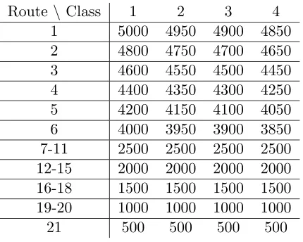
Table 3.3: Call arrival rates in the simulated network.
Route\ Class 1 2 3 4
1 5000 4950 4900 4850
2 4800 4750 4700 4650
3 4600 4550 4500 4450
4 4400 4350 4300 4250
5 4200 4150 4100 4050
6 4000 3950 3900 3850
7-11 2500 2500 2500 2500 12-15 2000 2000 2000 2000 16-18 1500 1500 1500 1500 19-20 1000 1000 1000 1000
21 500 500 500 500
In the simulation model, all 21 possible routes are considered, that is , u = 1. . .21, and for each route assume there are 4 classes of traffic, that is, k = 1. . .4. The demands for sub-wavelength units of the four classes ared1= 2, d2 = 4, d3= 6,and d4 = 8.
Assume that the routes in Figure 1.1 are numbered from 1 to 21 from the top-left route to the very bottom one. For example, the route between the first and the second nodes to the left is route 1, the route between the first and the third nodes to the left is route 7, and the route that uses all of the links is route 21, and so on. The arrival rates (calls per second) are assigned as shown in Table 3.3.
The service rate for all calls is set to be 500 calls per second. Inter-arrival times and call duration for all call types are assumed to be exponentially distributed with the above rates.
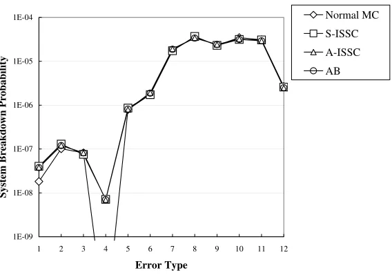
1E-09 1E-08 1E-07 1E-06 1E-05 1E-04
1 2 3 4 5 6 7 8 9 10 11 12
Error Type S y st em B re a k d o w n P ro b a b il it y Normal MC S-ISSC A-ISSC AB
Figure 3.3: Server breakdown probability caused by different kinds of error, λ=0.5.
A-ISSC method. The first 100,000 entry points of the ordinary simulation are used.
3.5.2 Simulation Results
Robust network server
Figure 3.3 and 3.4 show the server breakdown probability seen by each type of error under the two different service rates. From these figures, we can see that for λ= 0.5, the breakdown probability for error type 4 is too small for ordinary MC to estimate. In cases other than this, results from the all the simulation methods agree well with each other. Thus we can conclude that the methods we propose generate accurate and unbiased estimates.
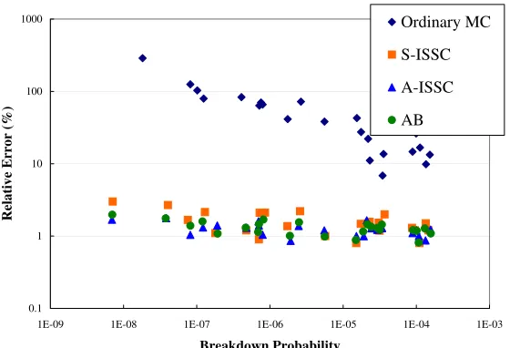
For the performance of these methods, Figure 3.5 shows the relative error, which is the standard deviation divided by the mean value of the estimate, versus the breakdown probabilities, for all the breakdown probabilities estimated in this system, including bothλ
1E-08 1E-07 1E-06 1E-05 1E-04 1E-03
1 2 3 4 5 6 7 8 9 10 11 12
Error Type S y st em B re a k d o w n P ro b a b il it y Normal MC S-ISSC A-ISSC AB
Figure 3.4: Server breakdown probability caused by different kinds of error,λ=1.
0.1 1 10 100 1000
1E-09 1E-08 1E-07 1E-06 1E-05 1E-04 1E-03
Breakdown Probability Relative Error (%) Ordinary MC S-ISSC A-ISSC AB
1E-25 1E-20 1E-15 1E-10 1E-05 1E+00
1 2 3 4 5 6
Route B lo ck in g P ro b a b il it y
Class 1, A-ISSC
Class 2, A-ISSC
Class 3, A-ISSC
Class 4, A-ISSC
Class 1, AB
Class 2, AB
Class 3, AB
Class 4, AB
Class 1, D-ISSC
Class 2, D-ISSC
Class 3, D-ISSC
Class 4, D-ISSC
Figure 3.6: Blocking probabilities for routes using one link.
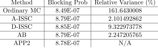
Table 3.4: Blocking probabilities and relative errors of Route 11, type 1. Method Blocking Prob Relative Variance (%)
Ordinary MC 8.49E-07 161.6430008
A-ISSC 8.79E-07 2.101492862
D-ISSC 8.85E-07 9.322973778
AB 8.79E-07 2.247205765
APP2 8.78E-07 N/A
AB method) has not been shown to have the BRE property.
From the efficiency point of view, since all three IS methods provide accurate estimates, the method that requires the least CPU time to generate an event would be the most preferable. Static ISSC would be the one in this case, since it does not require any extra effort to calculate the arrival rates throughout the simulation.
Traffic groomed optical network
1E-07 1E-06 1E-05 1E-04 1E-03 1E-02 1E-01
7 8 9 10 11
Route
B
lo
ck
in
g
P
ro
b
a
b
il
it
y
Class 1, A-ISSC
Class 2, A-ISSC
Class 3, A-ISSC Class 4, A-ISSC
Class 1, AB
Class 2, AB Class 3, AB
Class 4, AB
Class 1, D-ISSC Class 2, D-ISSC
Class 3, D-ISSC
Class 4, D-ISSC
Figure 3.7: Blocking probabilities for routes using two links.
Table 3.5: Blocking probabilities and relative errors of Route 11, type 2. Method Blocking Prob Relative Variance (%)
Ordinary MC 2.35E-06 117.2955219
A-ISSC 2.32E-06 1.750831756
D-ISSC 2.31E-06 8.386684392
AB 2.32E-06 1.863236585