Efficient steady-state solution techniques for variably saturated groundwater flow<

Efficient Steady-State Solution Techniques for

Variably Saturated Groundwater Flow

Matthew W. Farthing,

∗

Christopher E. Kees,

Todd S. Coffey,

C.T. Kelley

Cass T. Miller

a_{Center for the Advanced Study of the Environment, Department of}

Environmental Sciences and Engineering, University of North Carolina, Chapel

Hill, North Carolina 27599-7431, USA

b_{Center for Research in Scientific Computation, Department of Mathematics,}

North Carolina State University, Raleigh, North Carolina, 27695-8205, USA

c_{Mathematical Information and Computational Sciences, Sandia National}

Laboratories, Albuquerque, New Mexico, 87185-1110, USA

Abstract

We consider the simulation of steady-state variably saturated groundwater flow

us-ing Richards’ equation (RE). The difficulties associated with solvus-ing RE numerically

are well known. Most discretization approaches for RE lead to nonlinear systems

that are large and difficult to solve. The solution of nonlinear systems for

steady-state problems can be particularly challenging, since a good initial guess for the

steady-state solution is often hard to obtain, and the resulting linear systems may

be poorly scaled. Common approaches like Picard iteration or variations of

New-ton’s method have their advantages but perform poorly with standard globalization

techniques under certain conditions.

some time to obtain steady-state solutions for problems in which Newton’s method

with standard line-search strategies fails. It combines aspects of backward Euler time

integration and Newton’s method to select intermediate estimates of the

steady-state solution. Here, we examine the use of pseudo-transient continuation as well as

Newton’s method combined with standard globalization techniques for steady-state

problems in heterogeneous domains. We investigate the methods’ performance with

direct and preconditioned Krylov iterative linear solvers. We then make

recommen-dations for robust and efficient approaches to obtain steady-state solutions for RE

under a range of conditions.

Notation

Roman Letters

A accumulation term for pressure head form of RE

A accumulation term contribution to Jacobian

J Jacobian

C scaling factor for Dirichlet boundary conditions

F nonlinear function for DAE formulation, semi-discrete

G nonlinear function for DAE formulation, discrete

Ks saturated hydraulic conductivity

Ks

s surface saturated hydraulic conductivity

∗ _{Corresponding author}

Email addresses: matthew [email protected] (Matthew W. Farthing,),

chris [email protected](Christopher E. Kees,),[email protected] (Todd S.

Coffey,), tim [email protected](C.T. Kelley), casey [email protected](Cass T.

Ke effective hydraulic conductivity

Nmax maximum number of iterations for nonlinear solution methods

Od discrete spatial operator

R discrete spatial operator and source term

Se effective saturation

T extent of temporal domain

Xd extent of spatial domain along xd axis

f source term for the aqueous phase evaluated at cell centers

f source term for the aqueous phase

g gravitational vector

gu unit vector, g/kgk

ki intrinsic permeability

kr relative permeability

mv parameter for VGM

n unit outward normal for Ω

ne total number of nodes

nv parameter for VGM

nxd number of nodes along xd axis

p pressure of the aqueous phase

t time coordinate

u mass flux

ub _{Neumann boundary value}

ur _{precipitation rate}

y variable for DAE formulation

y0 _{temporal derivative for DAE formulation}

ymin lower bound for solution in test for evaluation error

Greek Letters

∆t time step for Ψtc methods

∆tmax maximum time step for Ψtc methods

∆xd spatial increment in xd direction

∆y Newton increment

Γ boundary of physical domain

ΓD portion of Γ for which Dirichlet boundary conditions are set

ΓN portion of Γ for which Neumann boundary conditions are set

Ω physical domain

αv parameter for VGM

β compressibility of the aqueous phase

²c switching tolerance in hybrid Newton-Picard method

²s sufficient decrease parameter for Armijo line search

θ volume fraction of the aqueous phase

θr residual volumetric water content

θs saturated volumetric water content

λ line-search scaling factor

λ+ intermediate scaling factor for quadratic line search µ viscosity of the aqueous phase

% density of the aqueous phase

ρ normalized density of the aqueous phase

σmin bound parameter for quadratic line search

σmax bound parameter for quadratic line search

τ TTE parameter for truncation error estimate bound

ψ pressure head

ψ0 _{initial condition for ψ}

Subscripts and Superscripts

d coordinate axis identifier (subscript)

i cell qualifier along x1 axis (subscript)

j cell qualifier along x2 axis (subscript)

l global identifier for solution unknowns (subscript)

n time level identifier (superscript)

sn nonlinear iteration index (superscript)

Abbreviations

Clock wall clock time (seconds) DAE differential algebraic equation Feval function evaluation

HAS two-level hybrid additive Schwarz domain decomposition precon-ditioner

Jeval Jacobian evaluation LF linear iteration failure LI linear iteration

LU-B banded LU decomposition from LAPACK

LU-S sparse LU decomposition from SPOOLES (version 2.2) NILS Newton’s method with a quadratic line search

NLF nonlinear iteration failure NLI nonlinear iteration

PIH Newton-Picard hybrid approach RE Richards’ equation

SER switched evolution relaxation Ψtc approach Steps attempted iterations for method

TTE temporal truncation errror Ψtc approach

VGM combined van Genuchten and Mualem p-S-k relation

p-S-k pressure-saturation-relative permeability constitutive relation Ψtc pseudo-transient continuation

1 Introduction

Variably saturated groundwater flow is commonly modeled using Richards’ equation (RE) along with a set of constitutive relations describing the interde-pendence among fluid pressures, saturations, and relative permeabilities (p-S

-k relations). While analytical and semi-analytical approximations for variably saturated flow exist, these are valid for limited sets of auxiliary conditions and domains [30]. As a result, significant effort has focused on developing robust techniques for solving RE numerically [9, 38, 29, 32, 27, 34, 36, 37]. Obtaining solutions for RE for many realistic physical conditions remains a challenge. Infiltration problems are often characterized by sharp fronts in both space and time. Steady-state solution is often nontrivial as well, since the volume fraction can vary steeply for problems with realistic boundary conditions and heterogeneous porous media.

associ-ated with resolving this nonlinear behavior have received attention. These in-clude solution variable transformations [4, 36], the evaluation ofp-S-krelations [33], approximation of interface conductivities in standard low-order spatial discretizations [38, 27], choice of dependent variable [37], and time discretiza-tion approach [9, 31, 33, 19]. Since the majority of time discretizadiscretiza-tions are implicit, both transient and steady-state problems typically lead to the solu-tion of a system of discrete nonlinear equasolu-tions. These systems can be quite large and difficult to solve, especially for problems with heterogeneous domains in two and three spatial dimensions.

The nonlinear system solution method used can then have a strong impact on the overall success of a simulator for RE. The most common approaches have been Picard iteration [9, 10, 19] or a variant of Newton’s method [34, 37, 21]. Each of these methods has its strengths and weaknesses, and several works have compared the robustness and efficiency of Picard and Newton approaches for a variety of problems [29, 25, 27, 8]. Newton’s method combined with glob-alization techniques like a line search, reduction of time step (backtracking), or the use of Picard iteration to obtain an initial guess has proven more reli-able and efficient than Picard iteration for several problems [29, 27]. However, both Newton and Picard approaches have been shown to perform poorly un-der certain conditions. The solution of nonlinear systems can be particularly difficult for steady-state problems due to the increased difficulty of obtaining a good initial guess for the steady-state solution. In addition, the scaling of the linearized systems is typically worse [15], and there is no longer recourse to reducing time steps when convergence breaks down [29].

Newton’s method with standard line-search strategies fails [23, 24, 11]. Ψtc combines features of backward Euler time integration and Newton’s method with the idea of using information about the transient physical problem to guide selection of intermediate iterates to the steady-state solution [15]. Since it uses information from a time-dependent problem, Ψtc can be more robust than standard line-search strategies, while incurring less computational ex-pense than full integration of the transient problem [23].

In this work, we seek effective techniques for obtaining steady-state solutions to RE. We examine the use of Ψtc methods as well as Newton’s method combined with standard globalization techniques for steady-state problems in homogeneous and heterogeneous domains. We investigate the methods’ per-formance with both direct and preconditioned Krylov iterative linear solvers. We then make recommendations for robust and efficient approaches to obtain steady-state solutions for RE under various conditions.

2 Background

is solved only approximately using, for example, a Krylov-type iterative linear solver [18]. Or, only an approximate Jacobian may be used in the Newton update. Common approaches for approximating the full Jacobian are to use finite differences (a numerical Jacobian) [14] or to lag its evaluation over a number of iterates (chord or modified Newton’s method) [33].

Like the hybrid Newton-Picard algorithm, Ψtc attempts to combine the rapid convergence of Newton’s method near the steady-state solution with a more robust iteration far from the solution. Ψtc employs a time-stepping approach when the iteration is far from the steady state, and thus exploits the rela-tionship between the nonlinear system for the steady-state problem and the initial value problem from which it is derived. The time-stepping algorithm used in Ψtc has properties similar to forward Euler with simple heuristics, which makes it both unstable and inaccurate as a time-integration method for stiff ordinary differential equations (ODE’s). Nevertheless, Ψtc can effectively maintain certain important qualities of the transient solution of some prob-lems such as enforcing a CFL condition, and has been shown to be effective in reaching the steady state for models with discontinuous transient phenomena such as shocks. While RE does not exhibit shocks under physically realistic choices of parameters, it does exhibit sharp fronts due to the nonlinearities as well as steep gradients due to discontinuities in the porous media properties.

3 Approach

3.1 Formulation

satu-rated conditions [26] gives

∂(ρθ)

∂t =∇ ·ρKe(∇ψ−ρgu) +f in Ω×[0, T] (1)

with

% =%0eβ(p−p0) ρ =%/%0 ψ = _% p

0kgk

gu = _kg_gk

Ks = %0k_µgkki

Ke =kr(ψ)Ks

(2)

Herep,%, andµare the pressure, density, and viscosity of the aqueous phase,

θis the volume fraction, andf is a source term for the aqueous phase.%0 is the density at p0,β is the compressibility of the aqueous phase, ψ is the pressure head, and g is a vector accounting for the acceleration of gravity. Ke is the

effective hydraulic conductivity, Ks is the saturated hydraulic conductivity,

and ki is the intrinsic permeability of the porous medium. Ω ⊂ IR2 is the

spatial domain, and [0, T] is the temporal domain.

The auxiliary conditions for eqn (1) are given by

ψ =ψb on ΓD, t∈[0, T] (3)

u·n=ub on ΓN, t∈[0, T] (4)

ψ =ψ0 in Ω, t= 0 (5)

where

is the mass flux,ψb_{, and u}b _{are boundary condition functions.ψ}0 _{is the initial}

condition, andnis the unit outward normal for Ω. We have also set Γ =∂Ω = ΓD∪ΓN with ΓD ∩ΓN =∅.

The steady-state form of eqn (1) is

−∇ ·ρKe(∇ψ−ρgu) = f in Ω (7)

with auxiliary data given by eqns (3) and (4) without temporal dependence. We use non-hysteretic forms of the p-S-k relations of van Genuchten [35] and Mualem [28] (VGM). For ψ <0, these are given by

Se=

(θ−θr)

(θs−θr)

(8)

Se= [1 + (αv|ψ|)nv]−mv (9)

kr=

q Se

h

1−(1−S1/mv

e )mv

i2

(10)

whereSeis the effective saturation,θris the residual volumetric water content,

θs is the saturated volumetric water content, αv is a parameter related to the

mean pore size, nv is a parameter related to the uniformity of the soil

pore-size distribution, and mv = 1−1/nv. For ψ ≥ 0, the porous medium is fully

saturated, and eqns (8)–(10) revert to

Se= 1 (11)

kr= 1 (12)

The pressure head form of RE is obtained from eqn (1) by applying the chain rule to the left hand side

A(ψ)∂ψ

A(ψ) =θ∂ρ ∂ψ +ρ

∂θ

∂ψ (13)

3.2 Spatial discretization

We consider a discretization of Ω = [0, X1]×[0, X2] ⊂ IR2 into a regular,

orthogonal grid with ne = nx1 ·nx2 nodes with ∆xd =Xd/(nxd−1), for d =

1,2. We apply a cell-centered finite difference approximation to the right hand side of eqn (1) and write for a cell Ωij in the interior,

∂(ρi,jθi,j)

∂t =−Ri,j (14)

Ri,j=−Od,i,j−fi,j (15)

i= 2, . . . , nx1−1, j = 2, . . . , nx2−1

For a cell Ωi,j in the interior, the discrete spatial approximation is

Od,i,j =

1 ∆x1

"

ρi+1/2,jKe,i+1/2,j

Ã

ψi+1,j−ψi,j

∆x1 −ρi+1/2,jgu1 !

− ρi−1/2,jKe,i−1/2,j

Ã

ψi,j−ψi−1,j

∆x1 −ρi−1/2,jgu1 ! #

+ 1 ∆x2

"

ρi,j+1/2Ke,i,j+1/2 Ã

ψi,j+1−ψi,j

∆x2

−ρi,j+1/2gu2 !

− ρi,j−1/2Ke,i,j−1/2 Ã

ψi,j−ψi,j−1

∆x2 −ρi,j−1/2gu2 ! #

(16) where the subscripts in g_u = [gu1, gu2]T indicate values for each coordinate,

and quantities with a 1/2 subscript denote values estimated at cell interfaces. For the interface values, we use a harmonic average for saturated hydraulic conductivity, the arithmetic average for density, and upwind the relative per-meability

Ke,i+1/2,j=kr,i+1/2,jKs,i+1/2,j

Ks,i+1/2,j= 2Ks,i,jKs,i+1,j/(Ks,i,j +Ks,i+1,j)

kr,i+1/2,j=

    

   

kr(ψi+1,j) if ψi+1_∆,j_x−₁ψi,j > ρi+1/2,jgu1 kr(ψi,j) otherwise

(18)

The corresponding terms along the other coordinate axis are defined symmet-rically.

The physical boundaries are located at the nodes (cell centers), so specify-ing Dirichlet conditions in pressure or volume fraction is straightforward. For example, at a cell Ωi,j ⊂ΓD, we set

C(ψi,j −ψi,jb ) = 0, (19)

whereCis a scaling factor that gives the boundary equation roughly the same scaling as the interior nodes.

For cells along ΓN, we use linear extrapolation to apply the flux at the exterior

(artificial) cell boundary rather than the cell center. This approach allows us to use the same nodal equation at the boundary node as we do at the interior points for Ωi,j ⊂ΓN. If, for example, Ω1,j ⊂ΓN, we set

u1,1/2,j =−2u1b,1,j−u1,3/2,j (20)

at the fictitious left cell boundary. Hereu = [u1, u2]T_.

3.3 Temporal approximation

finite difference spatial approximation to eqn (13) in a method of lines (MOL) context

A(ψi,j)

∂ψi,j

∂t =−Ri,j (21)

i= 2, . . . , nx1−1, j = 2, . . . , nx2−1

with the Dirichlet and Neumann boundary conditions given by eqns (19) and (20).

The semi-discrete system corresponding to eqn (21) can be written as a set of differential algebraic equations (DAE’s)

F(t,y,y0) = 0 (22)

whereFrepresents a set of equations that depend on timet, a set of dependent variables y, and a set of first-order derivatives with respect to time of these dependent variables,y0.

A variety of approaches can be used to integrate eqn (22). To illustrate the structure of the nonlinear system for transient problems, we use a backward Euler approximation to convert eqn (22) to a fully discrete system [13, 21].

G(tn+1,yn+1, 1

∆tn+1(y

n+1_−yn_{)) = 0 (23)}

3.3.1 Nonlinear solution for the transient problem

At each time level, a full time integration approach such as backward Euler must solve the nonlinear system eqn (23). A general Newton iteration for eqn (23) can be written

h

where {∆ysn+1} = {_yn+1,sn+1} − {_yn+1,sn} and s

n is a nonlinear iteration

index. The Jacobian, J, is formed by differentiating eqn (23) with respect to

y. For eqn (21), we can writeJ as

h

Jn+1,sni₌ 1

∆tn+1 h

An+1,sni₊

"

∂(Ay0)

∂y

n+1,sn# −

" ∂Od

∂y

n+1,sn#

(25)

where A is diagonal with [A]_l,l = A(ψi,j), ∂Ay0/∂y is also diagonal, and

∂O_d/∂ywill be banded with seven non-zero entries. Here,lis a global identifier corresponding to cell Ωi,j with, for example,l= (j−1)nx1+ifori= 1, . . . , nx1, j = 1, . . . , nx2.

For unknowns along ΓD,J is simply (see eqn (19))

h

Jn+1,sni

l,l =C (26)

3.4 Ψtc approximation

Ψtc attempts to find a solution to eqn (7) by integrating eqn (21) to steady state. The approach is straightforward and can included in many existing steady-state or transient solvers with minor modifications. The fully discrete Ψtc system can be obtained from eqn (21) by first applying a backward Euler time discretization as in eqn (23) and then using Newton’s method with yn

as the initial guess.

3.4.1 Solution for Ψtc update

(23) [23]. The resulting equation for the Ψtc iterate is

[Jn]n∆yn+1o=− {Rn}={Od(yn)}+{fn} (27)

with{∆yn+1}={yn+1} − {yn}since only one Newton iteration is performed and{yn+1,0_}={yn_{}.Jhas the same form as eqn (25), but without a derivative}

of the accumulation term

[Jn] = 1 ∆tn+1[A

n_]−

" ∂Od

∂y

n#

(28)

Note that when ∆t is small enough [Jn]≈ 1

∆tn+1[An] and therefore

∆yn+1 ≈ −∆tn+1[An]−1{Rn} (29)

which is the update corresponding to the forward Euler method applied to the ODE form of RE.

3.4.2 Ψtc step selection

Ψtc solves a series of problems of the form in eqn (27), while adapting the time step ∆tn+1 _{based on the intermediate solution’s behavior. There are a number}

of common strategies, for selecting ∆tn+1_{, including the switched evolution}

relaxation (SER) [23, 15, 11]

∆tn+1 = ∆tnkR

n−1_k

kRn_k (30)

so that ¯ ¯ ¯ ¯ ¯

(∆tn+1₎2

2(1 +|yn l|)

∂2_y

l

∂t2 (t

n₎ ¯ ¯ ¯ ¯ ¯

≤τ (31)

for each component of the solution yl and some constant τ. Here, we estimate

∂2_y

l/∂t2 attn by [11]

∂2_y

l

∂t2 (t

n_)≈ 2

∆tn_{+ ∆t}n−1 "

yn

l −yln−1

∆tn −

y_ln−1−yn_l−2

∆tn−1 #

(32)

For both SER and TTE, we also enforce an upper bound ∆tmax on the chosen

time step.

3.5 Newton’s method for the steady-state problem

Following eqn (21), we can write a cell-centered finite difference spatial ap-proximation of eqn (7) to solve the steady-state problem directly

Ri,j= 0 (33)

i= 2, . . . , nx1−1, j = 2, . . . , nx2 −1

with Dirichlet and Neumann boundary conditions given by eqns (19) and (20) without temporal dependence.

The Newton update for eqn (33) is

[Jsn_]n_∆ysn+1o_{=− {R}sn_}

[J] =− "

∂Od

∂y

#

3.5.1 Globalization techniques

A number of globalization strategies are commonly used to address the sensi-tivity of Newton’s method to initial guess. The Armijo line-search technique scales the original Newton update by a factor chosen to take a step as close to the original update as possible while insuring a sufficient decrease in the non-linear residual [18]. At iteration level sn for eqn (34), the Armijo line search

can be written

(1) Solve eqn (34) for ∆ysn+1_{, and set λ=λ+= 1}

(2) While kR(ysn+λ∆_ysn+1)k>(1−²

sλ)kR(ysn)k

Choose λ+

if λ+ < σminλ,λ+=σminλ

else if λ+> σmaxλ, λ+=σmaxλ

λ=λ+

(3) Set{ysn+1}₌{_ysn}_+λ{_∆ysn+1}

where ²s is a parameter controlling the amount of decrease required in the

nonlinear residual andλ is the final scaling factor. Here, we chose λ+ so that it minimized a three-point parabolic approximation ofkR(ysn_+λ∆ysn+1₎k₌

f(λ). Bounds onλ+are dictated byσminandσmax. The details of this approach

can be found in Kelley [22]. For this work we set σmin = 0.1,σmax = 0.55, and

²s = 10−4. The line search can fail if λ becomes too small. In this case, the

nonlinear solver is said to have failed due to line-search stagnation [11].

(1) Solve eqn (34) for ∆ysn+1, and set λ= 1

(2) While ysn

l +λ∆ysln+1 6∈[ymin, ymax] ∀l

λ=λ/2

(3) Set{ysn+1}={_ysn}+λ{∆_ysn+1}

In the numerical experiments presented below, we use an interval ymin =

−100 [m], ymax = 100 [m].

3.6 Picard iteration

Picard iteration has been used widely in the solution of RE [10, 19]. In brief, a Picard linearization of eqn (33) can be formulated as the Newton update in eqn (34) but with an approximate Jacobian in which the coefficient derivatives

∂kr/∂ψ and ∂ρ/∂ψ are omitted from ∂Od/∂y [29, 25]. The performance of

Picard iteration and Newton approaches have been compared in several works [29, 25, 27].

In many cases, Newton’s method with line search has proven more robust than a straightforward application of Picard iteration [27]. However, a hybrid Newton-Picard algorithm has also been suggested for reducing the sensitivity of Newton’s method to the quality of the initial guess [29, 8]. This approach performs an initial number of iterations for eqn (34) using the Picard approx-imation for J and then switches to a Newton update with the full Jacobian [29, 8]. The motivation for this approach is that the Picard iterations are, in general, cheaper than their Newton counterparts.

of Picard iterations are performed; and, (2) upon switching,ysn is sufficiently

close to the true to solution that the asymptotic convergence rate for the Newton updates is realized. There are several possible criteria for determining the crossover from Picard to Newton iteration, including k∆ysn_{k < ²}

c [8].

Alternatively, one can base the switch on sufficient decrease in the initial residual,

kRsn+1_{k< ²}

ckR0k (35)

We use eqn (35) in the numerical results presented below.

3.7 Linear system solution

We test five algorithms for solving the linear systems arising in the nonlinear iteration. As a direct solver, we use both the banded LU decomposition from LAPACK (LU-B) [1], as well as the implementation of LU from the SPOOLES package (LU-S) [2, 3] in PETSc [6, 7, 5]. We also test the iterative method BiCGstab using ILU preconditioning with zero fill from PETSc (BiCGstab-ILU), and a two-level hybrid additive Schwarz domain decomposition method (BiCGstab-HAS) [17].

4 Results

4.1 Test problems

4.1.1 Problem 1: infiltration example

The first test problem is a relatively simple one-dimensional example and pro-vides a case where each of the methods should perform well. We consider each test case as a transient problem with a corresponding steady-state solution. The first example simulates infiltration in vertical domain Ω = [0, X1]. Initial conditions for the infiltration are set to static equilibrium with the water table, located at the bottom of the domain. Constant Dirichlet boundary conditions are set at the top so that the steady-state solution contains both saturated and unsaturated regions. Table 1 summarizes the relevant physical parameters and auxiliary conditions.

4.1.2 Problem 2: hillslope example

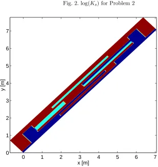
The spatial domain for the second problem, Ω = [0, X1]×[0, X2], is illustrated in Figure 1. The temporal domain is t ∈ [0, T] with T chosen so that the solution is at steady state. The relevant physical parameters and auxiliary conditions for Problem 2 are given in Tables 2-4. The log of the saturated hydraulic conductivity is given in Figure 2. Note that the domain is rotated 45 degrees to simulate a simple hillslope. The domain has block-heterogeneous medium properties ranging from clay to sand.

The boundary and initial conditions are configured to reflect an imperme-able bedrock at the X2− boundary, no flow at the X1+ boundary, and static,

Table 1

Fluid and domain properties for Problem 1

Variable Value Units

gu1 -1.0 [−]

kgk 7.321×1010 [m/d2]

%0 998.2 [kg/m3]

β 6.564×10−20 [m·d/kg]

p0 0 [kg/m·d]

X1 10 [m]

ψb(x1 = 0) 0 [m]

ψb(x1 = 10) -0.05 [m]

ψ0(x1) −x1 [m]

nv 4.264 [−]

αv 5.470 [m−1]

Ks 5.040 [m/d]

until the surface becomes saturated. After saturated conditions are reached at the surface, the outward normal flux increases to zero and becomes positive as the pressure rises above atmospheric pressure. This condition reflects a well-drained surface that permits very little ponding at the surface. The boundary conditions can be summarized as follows.

ψ_X−

1 =x2 (36)

ub_X+

1 = 0 (37)

ub_X−

2 = 0 (38)

ub_X+ 2 =         

ur_{, ψ <0}

ur_+Ks

sψ, ψ >0

         (39)

whereur _{is the precipitation rate andK}s

surface. For the numerical experiments presented,Ks

s = 10 [m/d]

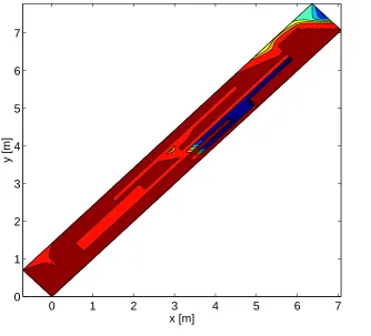
The steady-state solution of the volume fraction is given in Figure 3. This so-lution was computed by integrating the transient problem to T = 1700 [d] at which time kRk∞ <10−5. The solution was obtained using a DAE integrator

with relative and absolute integration tolerances of 10−4 _{[20, 21]. The}

tran-sient solution exhibits steep moving fronts throughout the domain while the equilibrium solution shown maintains a number of steep moisture gradients due to the layering of the media.

Fig. 1. Problem domain Ω

X+₁ X−₁

X+₂

X−₂

-6

x1 x2

(0,0)

(X1, X2)

4.2 Numerical experiments

Table 2

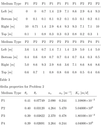
Media distribution for Problem 2

Medium Type P1 P2 P1 P1 P1 P1 P1 P2 P2 P2

Left [m] 0 0 0.7 1.4 2.9 7.1 8.6 2.9 6.4 9.3

Bottom [m] 0 0.1 0.1 0.1 0.2 0.1 0.3 0.1 0.2 0.1

Right [m] 10 0.71 1.4 2.9 6.4 9.3 9.3 7.1 7.1 10

Top [m] 0.1 1 0.8 0.3 0.3 0.3 0.8 0.2 0.3 1

Medium Type P2 P2 P2 P2 P2 P3 P3 P3 P4 P1

Left [m] 3.6 1.4 0.7 1.4 7.1 1.4 2.9 5.0 1.4 5.0

Bottom [m] 0.4 0.6 0.8 0.7 0.7 0.4 0.7 0.4 0.3 0.5

Right [m] 5.0 8.6 9.3 2.9 8.6 3.6 7.1 8.6 8.6 8.6

Top [m] 0.6 0.7 1 0.8 0.8 0.6 0.8 0.5 0.4 0.6

Table 3

Media properties for Problem 2

Medium Type θs θr nv αv [m−1] Ks [m/d]

P1 0.41 0.07749 2.090 0.244 1.10808×10−5

P2 0.40 0.03120 4.264 5.470 5.04000×100

P3 0.39 0.03822 2.370 0.478 1.80100×10−3

P4 0.39 0.02691 3.264 0.244 4.04000×100

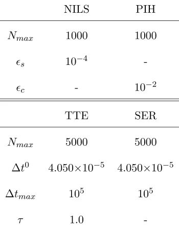
methods, SER and TTE, untilkRk2 <(kR0k2+ 1)10−5. The initial guess was

taken to be the initial conditions for the corresponding transient problem. For the NILS and PIH calculations, we enforced a maximum number of nonlinear iterations sn ≤ Nmax = 1000, while the maximum number of steps for the

SER and TTE runs was n ≤ Nmax = 5000. The maximum number of line

searches allowed was 1000 and the sufficient decrease parameter for Newton line search was ²s = 10−4. The PIH approach used a value of ²c = 10−2 in

Table 4

Fluid and domain properties for Problem 2

Variable Value Units

gu1 -0.7071 [−]

gu1 -0.7071 [−]

kgk 7.321×1010 [m/d2]

%0 998.2 [kg/m3]

β 6.564×10−20 [m·d/kg]

p0 0 [kg/m·d]

X1 10 [m]

X2 1 [m]

ur -0.4 [m/d]

Fig. 2. log(Ks) for Problem 2

0 1 2 3 4 5 6 7

0 1 2 3 4 5 6 7

x [m]

Fig. 3. Steady-state volume fraction for second test problem

0 1 2 3 4 5 6 7

0 1 2 3 4 5 6 7

x [m]

y [m]

of ∆t0 = 4.050 ×10−5, a maximum time step ∆tmax = 105, and the TTE

algorithm used τ = 1.0. The relevant parameters are summarized in Table 5.

The linear systems for Problem 1 were solved using the LU-B decomposition from LAPACK with each method. For Problem 2, we ran the numerical exper-iments for each of the four steady-state solution methods with the LU-S direct solver as well the two iterative methods (BiCGstab-ILU and BiCGstab-HAS). A relative residual test was used for BiCGstab with a tolerance of 10−6_{. The}

maximum number of linear iterations allowed was 2000 except where noted. The simulations were performed on a Pentium 4 (2.53 Ghz) workstation with 256 Mbytes of RAM running Redhat Linux 7.3. The elapsed time for the simulations was recorded using the ANSI C clock and time intrinsics.

Table 5

Numerical methods summary

NILS PIH

Nmax 1000 1000

²s 10−4

-²c - 10−2

TTE SER

Nmax 5000 5000

∆t0 4.050×10−5 4.050×10−5

∆tmax 105 105

τ 1.0

-Table 6. The labels are as follows:

• Jeval-Jacobian evaluation

• Feval-function evaluation

• Steps-attempted iterations for method

• NLI-nonlinear iteration

• NLF-nonlinear iteration failure

• LI-linear iteration

• LF-linear iteration failure

• Clock-wall clock time (seconds)

• X-failed to converge

Table 6

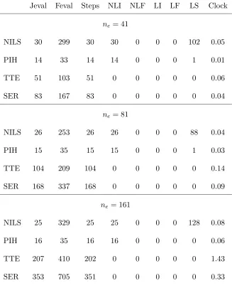
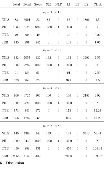
LU-B runs for Problem 1

Jeval Feval Steps NLI NLF LI LF LS Clock

ne = 41

NILS 30 299 30 30 0 0 0 102 0.05

PIH 14 33 14 14 0 0 0 1 0.01

TTE 51 103 51 0 0 0 0 0 0.06

SER 83 167 83 0 0 0 0 0 0.04

ne = 81

NILS 26 253 26 26 0 0 0 88 0.04

PIH 15 35 15 15 0 0 0 1 0.03

TTE 104 209 104 0 0 0 0 0 0.14

SER 168 337 168 0 0 0 0 0 0.09

ne= 161

NILS 25 329 25 25 0 0 0 128 0.08

PIH 16 35 16 16 0 0 0 0 0.06

TTE 207 410 202 0 0 0 0 0 1.43

SER 353 705 351 0 0 0 0 0 0.33

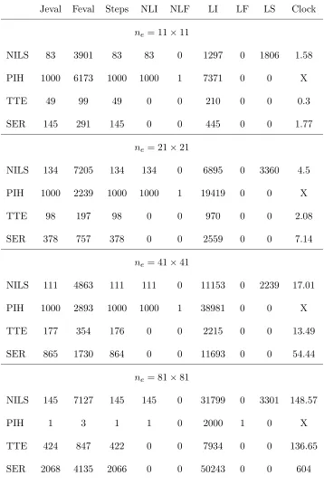
Problem 2 was more challenging than Problem 1 due to its dimensionality, het-erogeneous medium, and the nonlinear boundary condition at the surface. Re-sults of the numerical experiments with LU-S and BiCGstab are presented in Tables 7-9. The increased wall clock times, iteration counts, and line searches reflect the added difficulty of Problem 2. NILS converged for every linear solver and spatial grid in Tables 7-9. It required a similar number of nonlinear itera-tions and line searches for a particular grid, regardless of the linear solver used. Unlike NILS, PIH failed for the cases considered. With one exception where it failed in the initial linear solve, PIH did not reduce the original nonlinear residual sufficiently to satisfy eqn (35) and switch to NILS. In these cases, it exhausted the allowed number of nonlinear iterations.

Both the Ψtc methods converged for each spatial grid and linear solver com-bination in Tables 7-9, with TTE consistently between 2 and 5 times faster than SER. The run times for NILS and TTE were similar for most of the sim-ulations. NILS was more efficient with the LU-S solver, particularly for the 81×81 grid. On the other hand, TTE was more efficient for the BiCGstab calculations. The difference in run times increased for the HAS preconditioner, where TTE was 3 and 1.4 times faster than NILS on the 41×41 and 81×81 grids respectively.

The results also indicate a difference in the way NILS and TTE behaved as the spatial grid was refined. Namely, NILS required roughly the same number of iterations to converge regardless of spatial grid or linear solver, while the number of steps taken by TTE grew noticeably asne increased. To investigate

the performance of TTE, we ran an additional set of calculations whereτ was set to 10−3 _{and scaled by n}

e for each grid. The corresponding τ values ranged

result, the TTE time step selection was slightly more conservative on coarser grids than the original choice of τ = 1 and was more aggressive on the finer grids. Table 10 contains the results for TTE with LU-S and BiCGstab for

ne = 11×11 to ne = 161×161 as well as the results for NILS on the finest

grid.

With the use of a scaledτ, Steps for TTE was roughly the same forne= 11×11

to ne = 81×81 and each linear solver. There was still, however, an increase

in the number of steps for the finest grid, particularly for the BiCGstab-ILU solver. TTE with the scaled τ took slightly longer than the original τ = 1 calculations on the coarser grids, but reduced the total simulation time as the grids were refined. There was a corresponding improvement for TTE on the larger spatial grids with all three solvers. The computational effort for NILS and TTE withτ scaled was essentially the same for LU-S except for the finest grid, where NILS was 1.6 times faster. For ILU and BiCGstab-HAS, TTE with τ scaled was twice as fast as the simulations with τ = 1 on the ne= 81×81 grid.

We also note that BiCGstab-ILU did not perform well with the ne = 161×

161 system. Simulations with each of the steady-state solution methods and BiCGstab-ILU typically required significantly less computational effort than BiCGstab-HAS for the coarser grids. However, for ne = 161×161 the total

number of steps, linear iterations, and simulation time increased significantly for TTE while NILS failed after both 2000 and 10000 linear iterations.

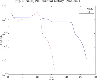
As an example of the progress of the Ψtc iterations in comparison to the Newton and Newton-Picard iterations, we graphed the history ofkRk2 versus

Fig. 4. NILS/PIH residual history, Problem 1

0 5 10 15 20 25 30

10−9 10−7 10−5 10−3 10−1 101

iterate

||R||

2

/||R

0

||2

NILS PIH

5. As it neared the steady-state solution, the method’s convergence steepened. This reflects the convergence of the Newton iteration that Ψtc reduces to near the root. Unlike the globalized Newton iteration, however, Ψtc does not enforce a decreasing sequence of residuals, and Figure 5 shows increased residuals at some points in the SER calculations. The iteration history of TTE was more extreme, often oscillating wildly before nearing the steady-state solution. Figure 6 shows the TTE calculation with τ = 1 on the ne = 81×81 grid.

Table 7

LU-S runs for Problem 2

Jeval Feval Steps NLI NLF LI LF LS Clock

ne= 11×11

NILS 83 3901 83 83 0 83 0 1806 1.5

PIH 1000 6173 1000 1000 1 1000 0 0 X

TTE 49 99 49 0 0 49 0 0 0.26

SER 145 291 145 0 0 145 0 0 1.65

ne= 21×21

NILS 132 7057 132 132 0 132 0 3291 2.55

PIH 1000 2239 1000 1000 1 1000 0 0 X

TTE 91 183 91 0 0 91 0 0 2.59

SER 379 759 379 0 0 379 0 0 7.5

ne= 41×41

NILS 106 4725 106 106 0 106 0 2181 9.92

PIH 1000 2885 1000 1000 1 1000 0 0 X

TTE 173 346 172 0 0 173 0 0 12.23

SER 866 1732 865 0 0 866 0 0 53.29

ne= 81×81

NILS 149 7369 149 149 0 149 0 3412 56.44

PIH 1000 3449 1000 1000 1 1000 0 0 X

TTE 450 888 437 0 0 450 0 0 164.43

SER 2068 4135 2066 0 0 2068 0 0 709.67

5 Discussion

Table 8

BiCGstab-ILU runs for Problem 2

Jeval Feval Steps NLI NLF LI LF LS Clock

ne= 11×11

NILS 83 3901 83 83 0 1297 0 1806 1.58

PIH 1000 6173 1000 1000 1 7371 0 0 X

TTE 49 99 49 0 0 210 0 0 0.3

SER 145 291 145 0 0 445 0 0 1.77

ne= 21×21

NILS 134 7205 134 134 0 6895 0 3360 4.5

PIH 1000 2239 1000 1000 1 19419 0 0 X

TTE 98 197 98 0 0 970 0 0 2.08

SER 378 757 378 0 0 2559 0 0 7.14

ne= 41×41

NILS 111 4863 111 111 0 11153 0 2239 17.01

PIH 1000 2893 1000 1000 1 38981 0 0 X

TTE 177 354 176 0 0 2215 0 0 13.49

SER 865 1730 864 0 0 11693 0 0 54.44

ne= 81×81

NILS 145 7127 145 145 0 31799 0 3301 148.57

PIH 1 3 1 1 0 2000 1 0 X

TTE 424 847 422 0 0 7934 0 0 136.65

SER 2068 4135 2066 0 0 50243 0 0 604

two-Table 9

BiCGstab-HAS runs for Problem 2

Jeval Feval Steps NLI NLF LI LF LS Clock

ne = 11×11

NILS 84 3959 84 84 0 4200 0 1833 1.13

PIH 1000 6173 1000 1000 1 24663 0 0 X

TTE 49 99 49 0 0 425 0 0 0.38

SER 146 293 146 0 0 1076 0 0 1.99

ne = 21×21

NILS 131 7059 131 131 0 46899 0 3293 26.3

PIH 1000 2239 1000 1000 1 51097 0 0 X

TTE 88 177 88 0 0 1628 0 0 2.63

SER 379 759 379 0 0 5799 0 0 9.04

ne = 41×41

NILS 110 4991 110 110 0 24471 0 2305 69.02

PIH 1000 3019 1000 1000 1 74767 0 0 X

TTE 168 336 167 0 0 4814 0 0 23.93

SER 866 1732 865 0 0 26241 0 0 117.69

ne = 81×81

NILS 148 7315 148 148 0 30762 0 3389 395.15

PIH 1000 3449 1000 1000 1 69639 0 0 X

TTE 439 867 427 0 0 11964 0 0 288.42

SER 2068 4135 2066 0 0 78706 0 0 1377.61

dimensional variably saturated flow problems examined in this work.

Table 10

Runs withτ scaled by ne for Problem 2

ne Jeval Feval Steps NLI NLF LI LF LS Clock

LU-S

TTE 11×11 114 229 114 0 0 114 0 0 1.57

TTE 21×21 127 255 127 0 0 127 0 0 2.96

TTE 41×41 125 250 124 0 0 125 0 0 8.16

TTE 81×81 146 281 134 0 0 146 0 0 58

TTE 161×161 248 458 209 0 0 248 0 0 667.07

NILS 161×161 232 12961 232 232 0 232 0 6043 429.58

BiCGstab-ILU

TTE 11×11 113 227 113 0 0 447 0 0 0.69

TTE 21×21 129 259 129 0 0 1132 0 0 2.36

TTE 41×41 130 260 129 0 0 1739 0 0 9.72

TTE 81×81 148 289 140 0 0 3474 0 0 65.85

TTE 161×161 806 1185 378 0 0 92232 0 0 2330

NILS 161×161 1 3 1 1 0 10000 1 0 X

BiCGstab-HAS

TTE 11×11 115 231 115 0 0 979 0 0 1.86

TTE 21×21 125 251 125 0 0 2173 0 0 4.28

TTE 41×41 131 262 130 0 0 3782 0 0 18.17

TTE 81×81 152 288 135 0 0 7192 0 0 131.9

TTE 161×161 283 472 188 0 0 20806 0 0 1386.07

Fig. 5. SER residual history, Problem 2

0 500 1000 1500 2000 2500 10−12

10−10 10−8 10−6 10−4 10−2 100

step

||R||

2

/||R

0

||2

Fig. 6. TTE residual history, Problem 2

0 50 100 150 200 250 300 350 400 450 10−12

10−10 10−8 10−6 10−4 10−2 100

step

||R||

2

/||R

0

||2

the conductivity was homogeneous. The resulting linear systems were also small and tridiagonal. Under these ideal conditions, NILS had little difficulty, and PIH was able to speed convergence to the steady-state solution. The Ψtc methods offered no benefit in this situation.

The methods’ relative performance changed though, as we moved to more re-alistic conditions. The controlling factor in their performance for Problem 2 was the difficulty associated with solving the resulting linear systems for each method. In addition to nonlinear boundary conditions, Problem 2 involved a two-dimensional, block-heterogeneous domain with medium properties corre-sponding to sand and clay. As a result, the linear systems for Problem 2 were more poorly scaled than in Problem 1. On the first step of the 81×81 grid the condition number of the NILS Jacobian was approximately 1019 _{and after 150}

iterations was 109 _{(condition numbers calculated using the dgbtrf/dgbcon}

routines from LAPACK).

The PIH approach did not perform as it was intended for Problem 2 because the initial Picard iterations did not adequately reduce the initial residual. The convergence of PIH could have been improved by relaxing the switching criterion in eqn (35) or enforcing a maximum number of Picard iterations, so that it would have switched to the Newton updates before exhausting the allowed iterations. However, this would be, in essence, just NILS and would have masked the ineffectiveness of the initial Picard iterations for Problem 2. In contrast, SER was robust but relatively inefficient. It converged for each of the runs and linear solvers, but was significantly slower than TTE for most cases. The two most efficient methods for Problem 2 were NILS and TTE. Their relative efficiency was dictated largely by the computational expense associated with the linear solvers. With both methods, the number of steps required for a given spatial grid was similar using the LU-S and BiCGstab solvers. However, the computational effort required changed significantly. Us-ing a robust direct solver, NILS was three time faster than TTE with τ = 1 on the 81×81 grid. However, it required four times as many total linear itera-tions with BiCGstab-ILU and three times as many using BiCGstab-HAS. As a result, it was 9% slower using ILU and 28% slower using BiCGstab-HAS.

The total number of iterations for NILS was fairly consistent on the spatial grids considered. On the other hand, TTE with τ = 1 did not scale as well when the spatial grids were refined. The total number of steps required to converge increased withne, making TTE more expensive. Varying τ based on

ne led to more consistent results for TTE and improved its performance for

the finer grids using the iterative linear solvers and converged for BiCGstab-ILU on the 161×161 grid when NILS failed.

The value of a number of parameters like²c, ²s, σmin, σmaxand the linear solver

tolerances for BiCGstab effected each of the methods considered to some de-gree. The performance of TTE for different τ values demonstrates that the the impact of parameter choices can be significant at times. Finding a suc-cessful configuration for a given method and problem usually requires some effort. While different choices of parameter values may lead to improved per-formance, the basic behavior of the methods was the same for the range of parameters we investigated. NILS was preferable for the simulations with a robust direct solver like LU-S, but BiCGstab performed better with the Ψtc algorithms. TTE was more aggressive than SER and more efficient than NILS when BiCGstab was used with either ILU or HAS preconditioning.

As a reference point, we also compared the performance of the Ψtc methods to time-accurate integration using a variable-order, variable step-size DAE integrator [20]. As might be expected, the full time integration was the most reliable approach for obtaining steady-state solutions, but the computational expense incurred was from 5 to 25 times greater than that of SER, which was similarly robust.

meth-ods for problems where good initial guesses for the steady-state solution are difficult to obtain.

The range of spatial grids presented for the numerical experiments was rela-tively coarse and the resulting linear systems were small to moderate in size. Still, the Jacobians were ill-conditioned for Problem 2, which proved to be a significant test for the direct and iterative linear solvers. For larger systems arising from realistic two and three-dimensional problems, we can only ex-pect the difficulties associated with the linear systems to become more severe. Moreover, large simulations will often have to be solved in parallel to obtain results in a reasonable timeframe. For the numerical experiments presented here, NILS combined with the LU-S solver was the most efficient approach on each spatial grid. However, preconditioned Krylov methods and sparse direct solvers have their own advantages and disadvantages depending on the prob-lem and architecture [12, 16]. A general comparison of their relative merits is beyond the scope of this paper.

6 Conclusions

Our numerical experiments for Ψtc approaches as well as Newton’s method with various globalization techniques lead us to the following conclusions and recommendations:

• For problems where use of a robust direct solver is feasible, Newton’s method with a line search is the most efficient approach for obtaining steady-state solutions to RE.

search can improve performance in some instances, but it does not neces-sarily lead to more robust performance for difficult problems.

• Inexact Newton methods with standard globalization techniques have par-ticular difficulty when the Jacobian is poorly scaled due to factors such as heterogeneous conductivity fields.

• If Newton’s method fails or performs poorly for a given steady-state prob-lem, it is worth examining a range of linear solver and line-search parameters before abandoning a Newton approach.

• Ψtc is a relatively simple approach that can improve the efficiency and robustness of existing steady-state solvers for RE on difficult problems, par-ticularly if iterative linear solvers are used.

Acknowledgments

The authors would like to thank Dr. T.-C. Yeh for several helpful suggestions. The research of CEK and CTK was supported in part by National Science Foundation grants DMS-0070641, DMS-0112542, and Army Research Office grant DAAD19-02-1-0391. The efforts of MWF and CTM were supported by grants 5 P42 ES05948 from the National Institute of Environmental Health Sciences and DMS-0112653 from the National Science Foundation. Computa-tional support was provided by the North Carolina Supercomputer Center.

References

D. Sorensen. LAPACK Users’ Guide. SIAM, Philadelphia, PA, 1992. [2] C. Ashcraft and R. Grimes. Spooles: An object-oriented sparse matrix

li-brary. InProceedings of the 1999 SIAM Conference on Parallel Processing for Scientific Computing. SIAM, 1999. March 22-24, San Antonio. [3] C. Ashcraft and R. Grimes. SPOOLES homepage. Technical Report

http://www.netlib.org/linalg/spooles/spooles.2.2.html, 1999.

[4] R.G. Baca, J.N. Chung, and D.J. Mulla. Mixed transform finite element method for solving the non-linear equation for flow in variably saturated porous media. International journal for numerical methods in fluids, 24: 441–455, 1997.

[5] S. Balay, W.D. Gropp, L.C. McInnes, and B.F. Smith. Efficient man-agement of parallelism in object oriented numerical software libraries. In E. Arge, A. M. Bruaset, and H. P. Langtangen, editors,Modern Software Tools in Scientific Computing, pages 163–202. Birkhauser, Boston, MA, 1997.

[6] S. Balay, W.D. Gropp, L.C. McInnes, and B.F. Smith. PETSc homepage. Technical Report http://www.mcs.anl.gov/petsc, Argonne National Lab-oratory, 1998.

[7] S. Balay, W.D. Gropp, L.C. McInnes, and B.F. Smith. PETSc 2.0 users manual. Technical Report ANL-95/11- Revision 2.0.28, Argonne National Laboratory, 2000.

[8] L. Bergamaschi and M. Putti. Mixed finite elements and Newton-type linearization for the solution of Richards’ equation. International journal for numerical methods in engineering, 45:1025–1046, 1999.

[10] L. M. Chounet, D. Hilhorst, C. Jouron, Y. Kelanemer, and P. Nicolas. Simulation of water flow and heat transfer in soils by means of a mixed fi-nite element method.Advances in Water Resources, 22(5):445–460, 1999. [11] Todd S. Coffey. Temporal and pseudo-temporal numerical integration methods. PhD thesis, North Carolina State University, Raleigh, NC, 2002. [12] I.S. Duff and H.A. van der Vorst. Developments and trends in the paral-lel solution of linear systems. Parallel Computing, 25(13–14):1931–1970, 1999.

[13] M. W. Farthing, C. E. Kees, and C. T. Miller. Mixed finite element methods and higher-order temporal approximations. Advances in Water Resources, 25(1):85–101, 2002.

[14] P.A. Forsyth, Y.-S. Wu, and K. Pruess. Robust numerical methods for saturated-unsaturated flow with dry initial conditions in heterogeneous media. Advances in Water Resources, 18:25–38, 1995.

[15] W.D. Gropp, D.E. Keyes, L. C. McInnes, and M. D. Tidriri. Globalized Newton-Krylov-Schwarz algorithms and software for parallel implicit cfd.

International Journal of High Performance Computing Applications, 14 (2):102–136, 2000.

[16] A Gupta. Recent advances in direct methods for solving unsymmetric sparse systems of linear equations.Association for Computing Machinery, Transactions on Mathematical Software, 28(3):301–324, 2002.

[17] E. W. Jenkins, C. E. Kees, C. T. Kelley, and C. T. Miller. An aggregation-based domain decomposition preconditioner for groundwater flow. SIAM Journal on Scientific Computing, 23(2):430–441, 2001.

[19] D. Kavetski, P. Binning, and S.W. Sloan. Adaptive time stepping and error control in a mass conservative numerical solution of the mixed form of Richards’ equation. Advances in Water Resources, 24:595–605, 2001. [20] C. E. Kees and C. T. Miller. C++ implementations of numerical

meth-ods for solving differential-algebraic equations: Design and optimization considerations. Association for Computing Machinery, Transactions on Mathematical Software, 25(4):377–403, 1999.

[21] C.E. Kees and C.T. Miller. Higher order time integration methods for two-phase flow. Advances in Water Resources, 25(2):159–177, 2002. [22] C. T. Kelley. Iterative Methods for Linear and Nonlinear Equations.

SIAM, Philadelphia, 1995.

[23] C.T. Kelley and D.E. Keyes. Convergence analysis of pseudo-transient continuation. SIAM Journal on Numerical Analysis, 35(2):508–523, 1998. [24] D.A. Knoll and P.R. McHugh. Enhanced nonlinear iterative techniques applied to nonequilibrium plasma flow. SIAM Journal on Scientific Com-puting, 19(1):291–301, 1998.

[25] F. Lehmann and Ph. Ackerer. Comparison of iterative methods for im-proved solutions of the fluid flow equation in partially saturated porous media. Transport in Porous Media, 31(3):275–292, 1998.

[26] C. T. Miller, G. Christakos, P. T. Imhoff, J. F. McBride, J. A. Pedit, and J. A. Trangenstein. Multiphase flow and transport modeling in hetero-geneous porous media: Challenges and approaches. Advances in Water Resources, 21(2):77–120, 1998.

[27] C. T. Miller, G. A. Williams, C. T. Kelley, and M. D. Tocci. Robust solution of Richards’ equation for non-uniform porous media. Water Re-sources Research, 34(10):2599–2610, 1998.

unsaturated porous media. Water Resources Research, 12(3):513–522, 1976.

[29] C. Paniconi and M. Putti. A comparison of Picard and Newton itera-tion in the numerical soluitera-tion of multidimensional variably saturated flow problems. Water Resources Research, 30(12):3357–3374, 1994.

[30] J.-Y. Parlange, W.L. Hogarth, D.A. Barry, M.B. Parlange, R. Haverkamp, P.J. Ross, T.S. Steenhuis, D.A. DiCarlo, and G. Katul. Analytical ap-proximations to the solution of Richards’ equation with applications to infiltration, ponding, and time compression approximation. Advances in Water Resources, 23:189–194, 1999.

[31] K. Rathfelder and L. M. Abriola. Mass conservative numerical solutions of the head-based Richards equation. Water Resources Research, 30(9): 2579–2586, 1994.

[32] J. Simunek, T. Vogel, and M. Th. van Genuchten. The SWMS 2D code for simulating water flow and solute transport in two-dimensional variably saturated media. Technical Report Research Report 132, U. S. Salinity Laboratory, Agricultural Research Service, U. S. Department of Agricul-ture, Riverside, CA, 1994.

[33] M. D. Tocci, C. T. Kelley, and C. T. Miller. Accurate and economical solution of the pressure-head form of Richards’ equation by the method of lines. Advances in Water Resources, 20(1):1–14, 1997.

[34] M. D. Tocci, C. T. Kelley, C. T. Miller, and C. E. Kees. Inexact Newton methods and the method of lines for solving Richards’ equation in two space dimensions. Computational Geosciences, 2(4):291–309, 1999. [35] M. Th. van Genuchten. A closed-form equation for predicting the

[36] G. A. Williams, C. T. Miller, and C. T. Kelley. Transformation ap-proaches for simulating flow in variably saturated porous media. Water Resources Research, 36(4):923–934, 2000.

[37] Y.-S. Wu and P.A. Forsyth. On the selection of primary variables in nu-merical formulation for modeling multiphase flow in porous media. Jour-nal of Contaminant Hydrology, 48:277–304, 2001.