Algorithm to Deblur Video Frame Using
Guided Filter
Vasavi Ennam, Prof. T. Ramashri
M.Tech Student, Dept. of ECE, S.V.U. College of Engineering, Tirupati, Andhra Pradesh, India
Professor, Dept. of ECE, S.V.U. College of Engineering, Tirupati, Andhra Pradesh, India
ABSTRACT: In recent days image processing is playing major role in research, especially to enhance and restore the
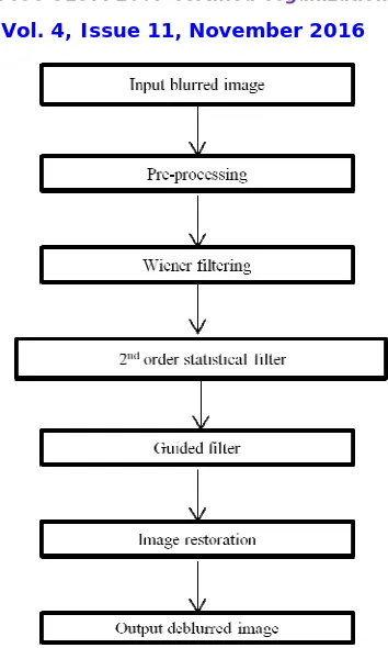
images for betterment of human perception for further analysis. This paper presents developed algorithm to deblur images or frames present in a video frames using guided filter to enhance the quality of visual perception to watch the video. Initially the blurred image is grabbed form video sequence, which is applied to wiener filter which restores the image, later on the output of wiener filter is applied to second order statistical filter to further bring out the blurred image near to original image. Finally the image is passed to guided filter to get the deblurred image near to original image suing matting laplacian kernel. The evaluation metrics need to know the performance of the developed algorithm is Peak Signal to Noise Ratio, Computational Complexity, and correlation factor.
KEYWORDS: Restoration, deblur, guided filter, peak signal to noise ratio, pictorial improvements, computational
complexity.
I. INTRODUCTION
Image processing is mostly used in applications like noise filtering, content enhancement which include contrast adjustment, reducing blurring effect for better visualization and remote sensing is used for filtering of Ariel image. It also has application in medical science like CT scan, brain tumor detection, cancer detection, ultra sonogram, etc. More specifically it is used in finger print recognition now a day it is also available in smart phones, weather forecasting, preserving boundary information, smoothing/sharpening of video or images etc.
Filtering is an image processing technique mostly used in computer vision, computer graphics, computational photography, etc. More specifically, filtering can be applied in many applications such as noise reduction, texture editing, detail smoothing/enhancement, tone mapping, haze/rain removal, and joint upsampling. Widely used technique is the edge-preserving bilateral filter [13] applied bilateral filter to image noise reduction and used bilateral filter on high dynamic range (HDR) images [1]. Also there are several other methods like joint bilateral filter, flash/no-flash denoising [5], etc use for filtering. Although a bilateral filter has a good edge-preserving characteristic, it has been noticed that it may have artifacts in detail decomposition and HDR compression. Artifacts are resulted from those pixels around the edge that may have an unstable Gaussian weighted sum [2]. To overcome this problem, a novel explicit guided filter is propose, which can filter output by considering the content of the guiding image. Guided filter is one of the spatial domain enhancement technique in which the filtering output is locally a linear transform of guidance image. Guided filter is much more than a smoothing. By using the content of guided image, it makes filtering output more structured and less smoothed than input. It can transfer the structure of the guidance image to the filtering output, enabling new filter applications such as dehazing and guided feathering.
ISSN(Online): 2320-9801 ISSN (Print): 2320-9798
I
nternational
J
ournal of
I
nnovative
R
esearch in
C
omputer
and
C
ommunication
E
ngineering
(An ISO 3297: 2007 Certified Organization)
Vol. 4, Issue 11, November 2016
II. RELATED WORK
The prevailing algorithm that aggregates a burst of snap shots (or a couple of burst for top dynamic range), taking what's much less blurred of everybody to construct an photograph that is sharper and less noisy than all of the pics within the burst. The algorithm is easy to put into effect and conceptually easy.
It takes as input a sequence of registered portraits and computes a weighted common of the Fourier coefficients of the image within the burst. Similar recommendations have been explored with the aid of Garrel et al. Within the context of astronomical portraits, where a pointy easy photo is made out of a video littered with atmospheric turbulence blur. With the availability of accurate gyroscope and accelerometers in, for example, phone cameras, the registration can be obtained “for free,” rendering the whole algorithm very efficient for on-board implementation. Indeed, one could envision a mode transparent to the user, where every time he/she takes a picture, it is actually a burst or multiple bursts with different parameters each. The set is then processed on the fly and only the result is saved. Related modes are currently available in “permanent open” cameras. The explicit computation of the blurring kernel, as commonly done in the literature, is completely avoided. This is not only an unimportant hidden variable for the task at hand, but as mentioned above, still leaves the ill-posed and computationally very expensive task of solving the inverse problem. Once the images are registered, the algorithm runs in O(M ・m ・ logm), where m = mh × mw is the number of image pixels and M the number of images in the burst. The heaviest part of the algorithm is the computation of M FFTs. Others propose to measure the local sharpness from the norm of the gradient or the image Laplacian. Joshi and Cohen [30] engineered a weighting scheme to balance noise reduction and sharpness preservation. The sharpness is measured through the intensity of the image Laplacian. They also proposed a local selectivity weight to reflect the fact that more averaging should be done in smooth regions. Haro and colleagues [31] explored similar ideas to fusion different acquisitions of painting images. The weights for combining the input images rely on a local sharpness measure based on the energy of the image gradient. The main disadvantage of these approaches is that they only rely on sharpness measures (which by the way is not necessarily trivial to estimate) and do not profit the fact that camera shake blur can be in different directions in different frames. Garrel et al. [7] introduced a selection scheme for astronomic images, based on the relative strength of signal for each spatial frequency in the Fourier domain. From a series of realistic image simulations, the authors showed that this procedure produces images of higher resolution and better signal to noise ratio than traditional lucky image fusion schemes. This procedure makes a much more efficient use of the information contained in each frame.
III.PROPOSED ALGORITHM
The Wiener filter is also called as the MSE-optimal stationary linear filter for images degraded by additive noise and blurring. A simplified equation of the Wiener filter R(u) is given below for the 1D case.
The inverse filter of a blurred image is a highpass filter. The parameter K of the Wiener filter is related to the low frequency aspect of the Wiener filter. The Wiener filter behaves as a as a bandpass filter, where the highpass filter is due to the inverse filter and the lowpass filter to the parameter K. Observe that when K=0, the Wiener filter becomes the inverse filter.
Figure 1:Flow Chart of research work
It takes into account the statistics of a region in the corresponding spatial neighborhood in the guidance image while calculating the value of the output pixel. Guided filter has good edge-preserving smoothing properties and does not suffer from the gradient reversal artifacts that are seen when using bilateral filter. It can perform better at the pixels near the edge when compared to bilateral filter.
The guided filter is also a more generic concept beyond smoothing. By using the guidance image, it makes the filtering output more structured and less smoothed than the input. It can transfer the structures of the guidance image to the filtering output, enabling new filtering applications such as guided feathering. Also, guided filter adopts the fast and non-approximation characteristics of linear time algorithm and provides an ideal option for real time applications in case of HD filtering. Hence, it is considered to be one of the fastest edge preserving filters. Guided filter generally has an ON time (in the number of pixels N) exact algorithm for both gray scale and color images, regardless of the kernel size and the range of intensity. ON time represents that the time complexity is independent of the window radius(r) and hence arbitrary kernel sizes can be used in the applications.
A. GUIDED FILTER:
Guided filter is a fast non-approximate linear-time algorithm which generates the filtering output by considering the content of a guidance image, which can be the input image itself or a different image. It is a low pass filter which implies for an input image, guided filter outputs its low frequency part.
The subtraction of low frequency part from the input image gives high frequency part of the image. This decomposition can be adjusted according to desired result by tuning degree of smoothness of guided filter.
The function of guided filter for an input image I can be realized as follows: I=I_L+I_H
ISSN(Online): 2320-9801 ISSN (Print): 2320-9798
I
nternational
J
ournal of
I
nnovative
R
esearch in
C
omputer
and
C
ommunication
E
ngineering
(An ISO 3297: 2007 Certified Organization)
Vol. 4, Issue 11, November 2016
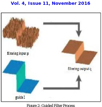
Figure 2: Guided Filter Process
It brings better results in denoising, image enhancement etc. Guided filtering algorithm can be applied only for gray scale images. Thus to perform it on color images, R, G, and B components are extracted and apply guided filter for each component.
IV.ALGORITHM
Step 1: Read the image say G, it acts as a guidance image Step 2: . Make I=G, where p acts as our filtering image.
Step 3: Enter the values assumed for r and ɛ, where r is the local window radius and ɛ is the regularization parameter. Step 4: Compute the mean of I, G, G*I
Step 5: The compute the covariance of (G,I) using the formula:-
cov_GI=mean_GI -meanG_.*mean_I
Step 6: Then compute the mean of (G*G) and use it to compute the variance using the formula:- var_G = mean_GG - mean_G .* mean_G
Step 7: Then compute the value of a, b. where a, b are the linear coefficients. Step 8: Then compute mean of both a and b.
Step 9: Finally obtain the filtered output image q by using the mean of a and b in the formula q = mean_a .* G + mean_b
V. RESULTS
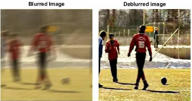
Figure 3: Input blurred image Figure 4: Output deblurred image
Performance Analysis:
PSNR Correlation Factor Computational Complexity
Blur removal using guided filter
73.182 0.8734 7
Existing method 40.506 0.9197 415
Table 1: comparison of proposed and existing methods
VI.CONCLUSION AND FUTURE WORK
In this paper, we proposed an efficient blur removal method for single image using guided filter. The guided filter sometimes introduces some negative effects. These effects are identified and resolved using some recovery methods. Our method is simple and it can effectively remove presence of blur from images. Even though our system brings good results for blur removal, it has to compromise some quality of image which can be resolved in future.
REFERENCES
[1] V. Bhateja, K. Rastori, A.Verma “A Non-Iterative Adaptive Median Filter for Image De-noising” IEEE conference on signal processing and Integration networks, pp. 113-118, 2014.
[2] Kaiming He, Jian Sun and Xiaoou Tang “Guided Image Filtering” IEEE Transation on Pattern Analysis and Machine Intelligence, vol. 35, no. 6, pp. 1397- 1409, June 2013.
ISSN(Online): 2320-9801 ISSN (Print): 2320-9798
I
nternational
J
ournal of
I
nnovative
R
esearch in
C
omputer
and
C
ommunication
E
ngineering
(An ISO 3297: 2007 Certified Organization)
Vol. 4, Issue 11, November 2016
[7] T. Buades, Y. Lou, J.-M. Morel, and Z. Tang, “A note on multi-image denoising,” in Proc. Int. Workshop Local Non-Local Approx. Image
Process. (LNLA), Aug. 2009, pp. 1–15.
[8] H. Zhang, D. Wipf, and Y. Zhang, “Multi-image blind deblurring using a coupled adaptive sparse prior,” in Proc. IEEE Conf. Comput. Vis.
Pattern Recognit. (CVPR), Jun. 2013, pp. 1051 1058.
[9] B. Carignan, J.-F. Daneault, and C. Duval, “Quantifying the importance of high frequency components on the amplitude of physiological tremor,”
Experim. Brain Res., vol. 202, no. 2, pp. 299–306, 2010.
[10] F. Gavant, L. Alacoque, A. Dupret, and D. David, “A physiological camera shake model for image stabilization systems,” in Proc. IEEE
Sensors, Oct. 2011, pp. 1461–1464.
[11] F. Xiao, A. Silverstein, and J. Farrell, “Camera-motion and effective spatial resolution,” in Proc. Int. Congr. Imag. Sci. (ICIS), 2006, pp. 33–36. [12] V. Garrel, O. Guyon, and P. Baudoz, “A highly efficient lucky imaging algorithm: Image synthesis based on Fourier amplitude selection,” Pub.
Astron. Soc. Pacific, vol. 124, no. 918, pp. 861–867, 2012.
[13] D. L. Fried, “Probability of getting a lucky short-exposure image throughturbulence,” J. Opt. Soc. Amer., vol. 68, no. 12, pp. 1651–1657, 1978. [14] D. Kundur and D. Hatzinakos, “Blind image deconvolution,” IEEE Signal Process. Mag., vol. 13, no. 3, pp. 43–64, May 1996.
[15] R. Fergus, B. Singh, A. Hertzmann, S. T. Roweis, and W. T. Freeman, “Removing camera shake from a single photograph,” ACM Trans.