ABSTRACT
VASANTH, ARJUN. Evaluation of Evapotranspiration-based and Soil-Moisture-based Irrigation Control in Turf. (Under the direction of Dr. Garry Grabow.)
Turfgrass is a major part of the landscape in North Carolina with its acreage equal to 44% of the state’s harvested crop acreage. Proper irrigation of residential, industrial and commercial turf areas is required to ensure healthy and acceptable turf quality. With
increasing competition for water resources and better turf quality, an efficient irrigation control technology is essential in meeting the dual goals of water conservation and turf
quality. The objective of the research was to compare two general types of commercially available irrigation control technologies; one based on estimates of evapotranspiration (ET) and the other based on feedback from soil moisture sensors. Water application and
turf quality resulting from using these technologies were compared to results from using a standard time-based irrigation schedule. The study also incorporated the effect of
irrigation frequency. The experimental area, located at North Carolina State University Lake Wheeler Turf Field Laboratories, Raleigh, North Carolina, consisted of forty 4-m x 4-m plots established to ‘Confederate’ tall fescue (Festuca arundinacea Schreb) using sod. There were ten treatments combining control type and watering frequency (3 technologies x 3 frequencies + 1 on-demand technology) with four replicates in a
randomized complete block design. Technologies included three systems: a time-based system, a soil-moisture-based “add-on” system, an ET-based system each with three frequencies: once per week, twice per week and seven days per week irrigation, and a
least amount of water while the ET-based technology applied the most water averaged
across frequencies. Once a week irrigation frequency applied the least amount of water, and daily irrigation frequency applied the most when averaged across all technologies. Minimally acceptable turf quality was met by all the treatments when averaged over the
duration of the study period, although during the last month of the study some technologies, especially the timer-based and add-on systems had noticeably drought
stressed plots. In general, the ET-based system and the water on-demand system had the best turf quality. The water on-demand system resulted in the best combination of water use efficiency and turf quality. Canopy temperatures were measured once a week and
there were significant differences in canopy temperature among treatments averaged over the season. The ET system plots had the lowest canopy temperature while the add-on
Evaluation of Evapotranspiration-based and Soil-Moisture-based Irrigation
Control in Turf
by
Arjun Vasanth
A thesis submitted to the Graduate Faculty of
North Carolina State University
in partial fulfillment of the
requirements for the Degree of
Master of Science
Biological and Agricultural Engineering
Raleigh, North Carolina
2008
APPROVED BY:
_______________________ _____________________
Dr. Rodney L Huffman Dr. Daniel C Bowman
_______________________ _____________________
Dr. Aziz Amoozegar Dr. Grady L Miller
___________________
Dr. Garry L Grabow
BIOGRAPHY
Arjun Vasanth was born on April 30th 1984 to Nalini Vasanth and Vasanth Narayanan in the city of Chennai, Tamil Nadu, India. He also has a younger sibling, Achyuthan Vasanth. He did his entire schooling in St Johns Senior Secondary school,
Chennai. After High School, Arjun attended Sri Venkateswara College of Engineering affiliated to Anna University, Chennai, India to pursue his Bachelors in Chemical Engineering. Working on his senior design project in wastewater treatment which seemed
to interest him, Arjun decided to enhance his knowledge by doing a Masters program in Environmental Engineering. He joined the Civil Engineering Department of North
Carolina State University to work on his Masters in July 2005. After two semesters of classes in the Civil Engineering department, he was offered a research assistantship position in the Biological and Agricultural Engineering Department to work on a turf
irrigation project. He joined the BAE Department in July 2006 and has been working on his Masters since then. Arjun is finishing his Masters in Biological and Agricultural
ACKNOWLEDGEMENTS
First of all I would like to thank my parents who have been a constant source of support to me and have backed me in all my endeavors. Next I would like to thank my committee members: Dr. Rodney Huffman, Dr. Dan Bowman, Dr. Grady Miller and Dr.
Aziz Amoozegar for all their help and useful suggestions during my research. A special thanks to Dr. Jason Osborne in the Statistics Department. Without his valuable advice my
analysis would never have been complete.
A big Thank You to Dr. Garry Grabow for giving me the opportunity to work for him. He has been a wonderful person, very supportive and helpful. Without his
suggestions, help and advice this whole research would not have materialized. It has been a great pleasure working for him.
I would like to acknowledge all the people who have helped me in my research and also like to thank all the graduate students in the BAE Department with whom I have had a good time in graduate school.
TABLE OF CONTENTS
LIST OF TABLES……… vi
LIST OF FIGURES……….………. vii
CHAPTER
1 INTRODUCTION……….………...………...……….. 11.1 Turfgrass Water Use and Management…....………...………….……….. 2
1.1.1 Effective Rainfall.……..………...……… 4
1.1.2 Reference Evapotranspiration.………...………... 5
1.1.3 Net and Gross Irrigation Requirement.……...…………...……… 8
1.2 Turfgrass Irrigation Control…...………..………... 8
1.2.1 Controller Clocks.…...……..……….………...……… 9
1.2.2 Soil Moisture measurement.………..………....……….………... 10
1.2.2.1 Time Domain Reflectometry……… 11
1.2.2.2 Frequency Domain Reflectometry……… 11
1.2.3 Evapotranspiration measurement...……….………...… 12
1.3 Smart Controllers….……....………... 13
1.3.1 Soil Water Sensor based control….………....…... 14
1.3.2 Evapotranspiration based control.……....………...………...…....…………... 15
1.4 Turf Quality..……..……… 16
2 MATERIALS AND METHODS……….……….…………... 18
2.1 Site and System Description…...……… 18
2.2 Experimental Design………...……….. 19
2.3 Uniformity Testing…………..……… 21
2.4 Technologies.…….………. 23
2.4.1 Standard time-based irrigation system..……….……….... 23
2.4.2 Soil Water Sensor based “add-on” irrigation system.……...…...……... 24
2.4.3 Soil Water Sensor based “water on-demand” irrigation system ……...…….. 24
2.4.4 Evapotranspiration based irrigation system……..………...….…... 25
2.5 Monitoring……….. 26
2.6 Data Analysis….………. 27
3 RESULTS AND DISCUSSION……...………... 38
3.1 Uniformity testing………... 38
3.2 Evaluation of the control technologies………... 39
3.2.2 Acclima add-on system……..……….….……….. 40
3.2.3 Acclima water on-demand system……….……… 42
3.2.4 ET controller system……….………. 42
3.2.5 Weekly applied water………..……….. 44
3.2.5.1 Technology comparison.………... 44
3.2.5.2 Frequency comparison..……… 44
3.2.5.3 Technology x Frequency comparison.….………. 44
3.2.6 Turf Quality…..……….… 45
3.2.6.1 Technology comparison……….…... 45
3.2.6.2 Frequency comparison……….……. 45
3.2.6.3 Technology x Frequency comparison……….……….. 46
3.2.7 Canopy temperature……..………. 49
3.2.7.1 Technology comparison……… 49
3.2.7.2 Frequency comparison……….. 49
3.2.7.3 Technology x Frequency comparison….……….. 50
3.3 Reference evapotranspiration from atmometer and Watchdog weather station……. 50
4 SUMMARY AND RECOMMENDATIONS...………... 72
REFERENCES………..………... 76
APPENDICES…..………...………. 81
Appendix 1 Weather data………...……….. 82
Appendix 2 SAS code used for Statistical Analysis …………..……….. 86
Appendix 3 Reference ET data from atmometer and Weather station…….………….... 93
LIST OF TABLES
Table Page Table 2.1 Monthly long-term reference ET, turf ET, precipitation, effective
precipitation, net irrigation requirement (NIR) and gross irrigation
requirement (GIR) (mm).………...………. 29
Table 2.2 Gross Irrigation Depth (mm) and runtime settings (minutes) for the Acclima add-on and time-based irrigation systems………...……… 29
Table 3.1 Uniformity testing results obtained on 23rd March 2007 before the start of the study……… 51 Table 3.2 Uniformity testing results done obtained on 16th October 2007 after the study... 51 Table 3.3 ANOVA for irrigation depth. Analysis done for data collected during 20 weeks.. 52
Table 3.4 Cumulative irrigation depth between 22nd April and 8th September 2007 (mm) and statistical comparison between treatments and frequencies………...…... 52
Table 3.5 ANOVA for turf quality data. Data collected over a 15-week period..………... 53 Table 3.6 Least square means estimates for turf quality ratings taken using a scale of
1 – 9 and statistical comparison between treatments and frequencies.…………... 53 Table 3.7 ANOVA for canopy temperature. Data collected over a 15-week period..……… 54
Table 3.8 Least square means estimates for canopy temperature (ºC) and statistical
comparison between treatments and frequencies……...……… 54
LIST OF FIGURES
Figure Page
Figure 2.1 Soil-water plot to determine field capacity………. 30
Figure 2.2 Inline 60 mesh filter at field site...….……….. 30
Figure 2.3 Water meter (AMCO Water Metering Systems Inc)….……….. 31
Figure 2.4 Campbell Scientific CR10X datalogger with switch closure module…..…... 31
Figure 2.5 Acclima RS500 module with sensor ……..……… 32
Figure 2.6 Acclima CS3500 water on-demand system ……….………... 32
Figure 2.7 Intellisense TIS240 ET controller ...….……….. 33
Figure 2.8 RS500 rain sensors...…………...……… 33
Figure 2.9 Schematic diagram of the plan view of the site showing plot layout and irrigation technologies………...………. 34
Figure 2.10 Relay Switches.………. 35
Figure 2.11 Anemometer………..……… 35
Figure 2.12 Shelter housing the controllers, transformer, relays and datalogger ……… 36
Figure 2.13 Uniformity testing using catch cans……...………... 36
Figure 2.14 Watchdog model 700 weather station….…………..……… 37
Figure 2.15 Atmometer with #30 canvas cover ….……….…. 37
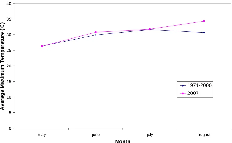
Figure 3.1 Monthly average maximum temperature (ºC) for May, June, July and August of 1971-2000 and 2007 against month……...………. 56
Figure 3.2 Average cumulative rainfall (mm) for the months of May, June, July and August of 1971-2000 and 2007 against month………...…. 56
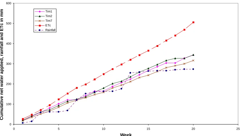
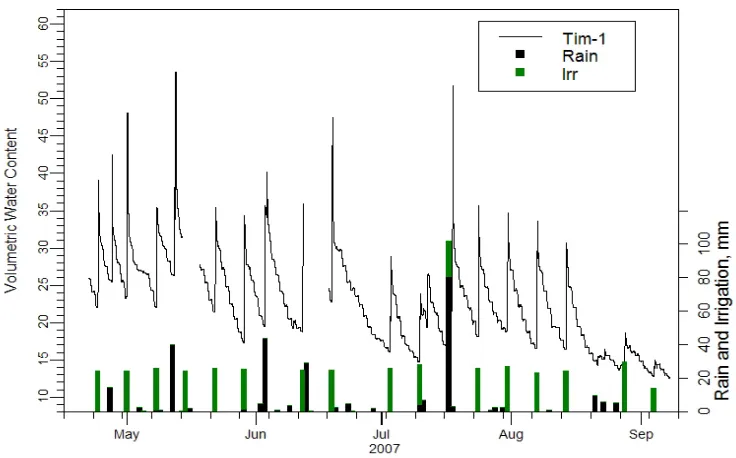
Figure 3.4 Crop evapotranspiration (ETc) and net applied water from the time-based technology..….……….………... 57 Figure 3.5 Soil-water content, rain and irrigation for the time-based controller set to irrigate once per week..…....………... 58 Figure 3.6 Soil-water content, rain and irrigation for the time-based controller set to irrigate twice per week….…….………... 58 Figure 3.7 Soil-water content, rain and irrigation for the time-based controller set to irrigate daily……….………... 59 Figure 3.8 Crop evapotranspiration (ETc) and net applied water from the soil-water- based technologies.…..………... 59 Figure 3.9 Soil-water content, rain and irrigation for the Acclima add-on system set to irrigate once per week..………... 60
Figure 3.10 Soil-water content, rain and irrigation for the Acclima add-on system set to irrigate twice per week..………...……….……… 60
Figure 3.11 Soil-water content, rain and irrigation for the Acclima add-on system set to irrigate daily………..……….... 61
Figure 3.12 Soil-water content, rain and irrigation for the Acclima on-demand
system………... 61
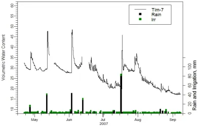
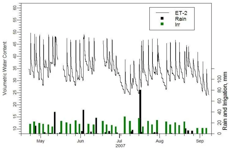
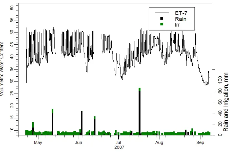
Figure 3.13 Soil-water content, rain and irrigation for the Intellisense TIS 240 controller set to irrigate once per week………....………..……… 62
Figure 3.14 Soil-water content, rain and irrigation for the Intellisense TIS 240 controller set to irrigate twice per week….………... 62 Figure 3.15 Soil-water content, rain and irrigation for the Intellisense TIS 240 controller set to irrigate daily.…....…..………. 63 Figure 3.16 ETc (from weather station) and net applied water from the ET-based
technology………. 63 Figure 3.17 Turf quality of plots in the lower terrace at the end of the experimental
Figure 3.18 Turf quality of plots in the upper terrace at the end of the experiment
period………...…. 64 Figure 3.19 Turf quality (average of 4 replications) for add-on and on-demand
Technologies………... 65 Figure 3.20 Turf quality (average of 4 replications) for time-based technology...…... 65
Figure 3.21 Turf quality (average of 4 replications) for ET based technology………… 66 Figure 3.22 Turf quality and canopy temperature against week for timer-based once per week treatment……… 66 Figure 3.23 Turf quality and canopy temperature for Acclima add-on system at once per week frequency………...……… 67 Figure 3.24 Turf quality and water applied against week for timer-based system at once per week frequency……….………. 67
Figure 3.25 Turf quality and water applied against week for Acclima add-on system at once per week frequency………...……... 68
Figure 3.26 Plot of canopy temperature of ET-7 and AC1-7 over time………... 68 Figure 3.27 Plot of canopy temperature of ET-7 and Tim-1 over time……… 69 Figure 3.28 Bivariate plot of the relationship in canopy temperature between AC2
and AC1-1 treatments………..……….. 69 Figure 3.29 Bivariate plot of the relationship in canopy temperature between AC2 and AC1-7 treatments……….……….. 70
Figure 3.30 Bivariate plot of the relationship in canopy temperature between AC2 and Tim1 treatments………...……….. 70
Figure 3.31 Bivariate plot of the relationship in canopy temperature between AC2 and Tim7 treatments……….. 71
CHAPTER 1
1. Introduction
Maintained turf acreage in North Carolina increased by 21.4% between 1995 and
1999 and homeowners accounted for 69% of the increase (NCDA, 2001). Turf irrigation
is also on the rise with 96% of the golf courses in NC using some sort of turf irrigation
(NCDA, 2001). The largest category of turf installation in the United States includes
single-family and multiple-family residences (Cockerham and Gibeault, 1985). Turfgrass
is a major part of the landscape in North Carolina with acreage equal to 44% of the
state’s harvested crop acreage (NCDA, 2001). More than 2.1 million acres of turfgrass
add to the functional, recreational and aesthetic value of the state.
Proper irrigation of residential, industrial and commercial turf areas is required to
ensure healthy and acceptable turf quality. With recurring drought problems, several
municipalities in North Carolina have imposed water-use restrictions limiting or banning
landscape irrigation. As of November 6th 2007, most of the counties in North Carolina are
classified under one of the following drought conditions; (D0) impending drought, (D1)
Moderate drought, (D2) Severe drought and (D3) Extreme drought. The city of Raleigh
restricted lawn watering to three days a week until 23rd October after which landscape
irrigation was banned. Charlotte, NC banned all landscape irrigation as of 24th September
2007. Efficient irrigation of landscape using new irrigation control technologies may help
1.1 Turfgrass Water Use and Management
Turfgrasses can be classified as cool-season turf or warm-season turf depending
on physiological processes. The most common cool-season turf includes tall fescue,
Kentucky bluegrass, perennial ryegrass and creeping bentgrass while the most common
warm-season turf are bermudagrass, zoysiagrass, St Augustinegrass, kikuyugrass,
centipedegrass and bahiagrass (Beard, 1985). Cool-season grasses grow well in the
northern United States. They grow actively in cool spring weather and slow down or go
dormant in the heat of summer when the temperature reaches 30º C. In areas with a hot
climate, tall fescue grows best when irrigated (NCDA, 2004). The improved turf-type tall
fescues are finding widespread acceptance as lawn grass in the transition zone of the US.
In the southern region under moderately shaded conditions, tall fescue is gaining in
popularity (Duble, 1996). Also, the improved tall fescues retain color during the winter
months providing a year-round green lawn.
Depending on the area’s climate, residential outdoor water use varies from 22% to
67% of the total water use of a household (Mayer et al., 1999). Recent studies in the US
reveal that 58% of potable water is used for landscape irrigation (Mayer et al., 1999). In
the same study, it was observed that homeowners used an average of 77 mm of water per
month for landscape irrigation in the US. However, Baum (2005) found that typical
homeowners in Florida used an average of 116 mm per month of water.
In a recent survey of five communities in North Carolina (within the Neuse River
89% in New Bern (Osmond and Hardy, 2004). The same study found that Cary, NC,
residents with fixed irrigation systems applied almost twice the amount of water as those
irrigating with movable sprinklers.
North Carolina receives an average of 1150 mm of rainfall a year (National
Oceanic and Atmospheric Administration [NOAA], 2003). Applying the same amount of
water at regular intervals, as with timer-based irrigation scheduling, will often result in
over-irrigation and the needless waste of water and energy. North Carolina with its humid
environment requires irrigation planned in conjunction with the prevailing rainfall
conditions to limit water waste and achieve the high quality landscapes desired by
homeowners.
Historically, NC guidelines for irrigation have been to irrigate 25 mm per week in
the absence of rain (Bruneau et al., 2000) although turfgrass water use can exceed 25 mm
during peak demand periods and be less during cool, cloudy days. Peacock and Bruneau
provided newer guidelines that indicated turfgrass water demand to be 48 mm per week
during the month of July and 18 mm per week in October.
In order to conserve water, and at the same time have a healthy turf, proper irrigation
scheduling (applying the right amount of water at the right time) is required. Irrigation
scheduling can be done in a number of ways to allow proper irrigation of turfgrass. The
practical methods of scheduling include: daily replacement, fixed day irrigation, fixed
amount irrigation, cycle start, soil-water balance checkbook and historical ET override
water holding capacity of the soil, root depth, effective rainfall and weather conditions
including temperature, solar radiation and wind speed.
Available water holding capacity (AWHC) is the fraction of soil-water that is
considered available for plant use and is measured in mm m-1 of the crop root zone.
Traditionally, AWHC is half of the total water content in the soil at field capacity (Allen
et al., 1998). This fraction varies for different types of soil. Field capacity is defined as
the amount of water held in the soil against the force of gravity after saturating the soil by
irrigation or rainfall. Gravity drainage starts with the largest pores draining rapidly. After
drainage decreases to a very slow rate, the water content of the soil measured at this point
is called the field capacity. It is not a definite water content but an approximation after
rapid drainage (Carrow, 1985) and generally speaking it is taken to be the water content
at soil-water tension of 0.1 bar (for sandy soil) or 0.33 bar (for clay-loam soil).
To prevent plant stress, irrigation should be scheduled before the soil-water level
drops below a certain percentage of field capacity known as the Management Allowable
Depletion (Smajstrla et al., 1989).
1.1.1 Effective Rainfall
Effective rainfall (ER) is that portion of total rainfall that plants use to help meet
their consumptive water requirements. It is an important component of irrigation
requirement estimation. An empirical formula for calculating ER given in SCS TR-21
(USDA, 1970) is
where
Pm = precipitation [mm],
ETc = crop evapotranspiration [mm day-1], and
SF = soil water storage factor calculated using the formula
SF 0.531747 0.295164 D 0.057697 D 0.003804 D (2)
where
D = usable soil water storage which is fraction of the available water holding capacity of
the soil. In this study, D was taken as 0.66 of the AWHC of the crop root zone.
1.1.2 Reference Evapotranspiration
Evapotranspiration (ET) is the process by which water is transferred to the
atmosphere through evaporation and transpiration. Evaporation is the physical process
whereby water is changed from a liquid to a gas from free water surfaces, such as ponds,
streams, and from wet soil or wet vegetation. Transpiration is a process where plants
exchange water for carbon dioxide. All leaves have microscopic openings, called
stomata. When open, water evaporates due to a concentration gradient. Carbon dioxide
can also diffuse into the plant through the open cavity. When the stomata close, little
carbon dioxide or water enters or leaves the plant. The plant balances the opening and
closing of the stomata to acquire enough carbon dioxide and not lose too much water, so
it can stay alive. Environmental conditions such as air temperature, humidity, radiation,
wind etc affect the evapotranspiration from plants.
crops. In general, there are two types of reference evapotranspiration; Grass reference
evapotranspiration (ETo) and alfalfa (Medicago sativa) reference evapotranspiration (ETR). According to Allen et al. (1998), reference evapotranspiration is defined as
“the rate of evapotranspiration from a large area, covered by green grass, 8 to 15 cm tall,
which grows actively, completely shades the ground and which is not short of water”.
Measurement of reference evapotranspiration is difficult so empirical equations
have been developed to estimate it. These include the Thornthwaite, Blaney-Criddle, and
the Penman-Montieth equations (Allen et al., 1998). Of these, the Penman-Montieth is
currently the most widely used.
In 1948, Penman combined energy balance with a mass transfer method to derive
an equation to compute the evaporation from an open water surface using temperature,
humidity, wind speed and solar radiation. This equation was further developed by many
researchers. Resistance to vapor flow was differentiated between bulk surface resistance
and aerodynamic resistance. The bulk surface resistance describes the resistance of vapor
flow through stomatal openings and the aerodynamic resistance describes the resistance
above the vegetation and includes friction from the air flowing above the vegetative
surface (Allen et al., 1998).
The FAO Penman-Montieth equation is
ET . ∆ R G∆ ⁄.T (3)
where
Rn = net radiation at the crop surface [MJ m-2 day-1],
G = soil heat flux density [MJ m-2 day-1],
T = mean daily air temperature at 2 m height [°C],
u2 = wind speed at 2 m height [m s-1],
es = saturation vapor pressure [kPa],
ea = actual vapor pressure [kPa],
es - ea = saturation vapor pressure deficit [kPa],
Δ = slope of the saturation vapor pressure curve [kPa °C-1], and
γ = psychrometric constant [kPa °C-1].
The amount of water required to replace evapotranspiration is termed the crop
water requirement, CWR. The CWR can be met by rain and irrigation. To obtain the crop
evapotranspiration (ETc), the reference evapotranspiration, ETo, is multiplied by a crop
coefficient, Kc (Allen et al., 1998):
ET ET K (4)
The effects of characteristics that distinguish field crops from grass are integrated
into the crop coefficient (Kc). The crop coefficient depends mainly on the type of crop,
the growth stage of crops and the climate (Allen et al., 1998). Crops like maize with a
high leaf area index can transpire more and hence require more water than a reference
crop while cucumber requires less water than the reference crop. Crops use more water
when fully developed than in the first weeks subsequent to planting. The climate
Heibloem, 1986). For this research a crop coefficient of 0.8 specific to cool-season
turfgrass was used (Allen et al., 1998).
1.1.3 Net and Gross Irrigation Requirement
The net irrigation requirement (NIR) is defined as the net amount of irrigation
water required to replace crop ET after accounting for effective rainfall:
NIR ET ER (5)
The gross irrigation requirement (GIR) is the quantity of water to be applied by
the irrigation system after accounting for irrigation uniformity (Allen, 1997):
GIR S UNIR (6)
The gross irrigation requirement can be computed daily, weekly, monthly and
seasonally. With the known sprinkler application rates and GIR, the irrigation runtimes
for the system can be calculated.
1.2 Turfgrass Irrigation Control
There is a steady increase in the number of people using residential irrigation
systems in North Carolina. Residences using irrigation systems increased by 29.4%
between 1994 and 1999 (NCDA, 2001). An efficient irrigation schedule is essential in
meeting the dual goals of water conservation and acceptable turf quality. Under-irrigation
and over-irrigation can negatively affect turfgrass quality (Cardenas-Lailhacar et al.,
2005). Over-irrigation results in waste of water and leaching of nutrients while
under-irrigation results in poor turf quality. In time-based under-irrigation, under-irrigation duration and
al. (2005) observed that by just adding a rain sensor to a time-based irrigation schedule
reduced water usage by 45%. Improved irrigation efficiency by using the correct amount
of water can be achieved by different methods.
1.2.1 Controller Clocks
Controller clock systems are an essential part of automated irrigation systems.
While electro-mechanical and mechanical controllers were commonly used in the early
1970’s, controllers became exclusively electronic in the 1990’s (Zazueta et al., 1993).
Even though these controllers offer means to schedule irrigation and control the amount
of water applied, they are only as good as the information used to program them. As
required knowledge and information are frequently lacking, most of the control clocks
are incorrectly programmed. There are two types of controller systems; open loop system
and closed loop system. In open loop systems, the operator decides on the amount of
water that will be applied and when the irrigation will occur. This information is
programmed into the controller and water is applied accordingly. Open loop systems
normally have a clock to start irrigation. In a closed loop system, the operator develops a
general control strategy using feedback from measurement instruments. Once the general
strategy is established, the control system takes over and makes detailed decisions of
when to apply water and how much to apply (Zazueta et al., 1993; Boman et al., 2002).
The simplest form of a closed loop irrigation system is an irrigation system that is
controlled by a soil-water sensor. The sensor is wired in series with an electrical solenoid
when the water content is above a set threshold prohibiting any pre-programmed
irrigation and closing the circuit when watering is needed.
1.2.2 Soil-Water Measurement
The most accurate method of measuring soil water content is the
thermogravimetric method, which requires heating a known mass of soil at 105º C for a
specific time and determining the weight loss. This method is time consuming and
destructive to the sampled soil.
Indirect methods of estimation of soil-water include tensiometry, electrical
conductivity, measurement of the bulk soil dielectric constant, gamma ray attenuation
and neutron thermalization. Various types of sensors such as tensiometers, granular
matrix sensors and time domain reflectometry probes have been used to provide feedback
in closed loop systems (Dukes and Scholberg, 2004; Blonquist et al., 2005; Boman et al.,
2002). A tensiometer is a device used to determine matric water potential Ψm (soil-water
tension) which is then related to the volumetric soil water content. A study conducted by
Neil and Carrow (1982) revealed that Kentucky bluegrass with tensiometer controlled
irrigation used 28 to 48 percent less water than time-based irrigation water use.
Granular matrix sensors are similar to tensiometers in that they are made of a
porous material that reaches equilibrium with the soil-water. The soil-water tension is
correlated to an electrical signal based on a calibration equation (Munoz-Carpena et al.,
2003). Granular matrix sensors have been used to automatically irrigate urban landscapes
feedback on corn and cotton in North Carolina (Grabow et al., 2004) and potatoes (Shock
et al., 2002).
There has been a significant advancement in the use of electromagnetic methods
in the measurement of soil-water content. Use of these electromagnetic methods coupled
with the use of computer technology has resulted in the establishment of inexpensive
soil-water sensors for automated irrigation of landscapes. There are two main techniques
involved, Time Domain Reflectometry (TDR) and Frequency Domain Reflectometry
(FDR; Charlesworth, 2000).
1.2.2.1 Time Domain Reflectometry
Time domain reflectometry instruments operate by sending an electromagnetic
signal through a pair of parallel rods buried in the soil. This pulse travels the length of the
rods and is reflected back to the control unit which detects and analyses it. The time taken
by the pulse to travel the length of the rod depends on the length of the rod and also the
dielectric constant of the moist soil. This is then related to the volumetric soil water
content. Time domain reflectometry has been used to initiate and terminate irrigation of
the plots based on soil-water measured by TDR probes installed at a depth of 13 cm
(Topp et al., 1984; Dukes and Scholberg, 2004). Time domain transmissivity (TDT)
probes are similar to TDR probes in operation but have less signal attenuation (assuming
sensor rods are the same length) and are more affordable (Blonquist et al., 2005).
1.2.2.2 Frequency Domain Reflectometry
placing the soil between two electrical plates. When a voltage is applied between the two
plates, a frequency is measured which varies with the dielectric constant of the soil
medium. And the dielectric constant of the moist soil is related to the volumetric soil
water content (Charlesworth, 2000).
1.2.3 Evapotranspiration Measurement
Standard irrigation controllers require users to input irrigation schedules and
adjust run-times in response to climatic conditions. Another type of system being used in
turfgrass irrigation control is based on controllers that use weather information to
estimate ET and adjust irrigation using a soil–water budget. These controllers commonly
called evapotranspiration controllers receive information from local or on-site weather
stations and adjust watering durations based on the climatic conditions.
An atmometer can be used to estimate ET as a substitute for ET estimated using
weather data. An atmometer is a device that includes a porous ceramic plate (Bellani
plate) that has been modified to make an inverted cup and is filled with distilled water. A
water filled supply tube is inserted through an opening of a rubber stopper that attaches to
the ceramic cup opening. The cup assembly is then mounted on top of a cylindrical
reservoir made of white polyvinyl chloride (PVC) filled with distilled water. The supply
tube extends into the cylindrical reservoir and establishes a continuous connection
between the water in the cup and the cylindrical reservoir below. Any water lost from the
cup by evaporation is replenished with water from the reservoir via the tube due to
glass tube connected by two ports to the reservoir and mounted outside the reservoir. A
scale is affixed on the outside wall of the cylindrical reservoir near the glass tube for
reading the amount of evaporation. Atmometer-measured evaporation adjusted with an
appropriate regression equation to obtain ET0 can be used in water balance calculations
for irrigation scheduling (Alam and Elliott, 2003). An atmometer with a dense fabric (#30
canvas) has been used to simulate grass-based ETo while a standard model with #54
green canvas is recommended for measuring alfalfa-based ETR (Alam and Trooein,
2001). Magliulo et al. (2003) found high values of correlation coefficient when
comparing ETo determined by an atmometer and a Penman Montieth equation based ETo.
Research done in Silsoe, United Kingdom, show that evaporation measured with an
ETgage (an atmometer made in Colorado, USA) was in close agreement with
Penman-Montieth ETo for grass reference (Hess, 1996).
1.3 Smart Controllers
Smart controllers can be broadly separated into two categories – those that use
feedback from a sensor to monitor the amount of water in the root zone and those that use
weather data to estimate amount of water required by the turf for irrigation. Automated
irrigation using these smart controllers has become the new trend in turf irrigation.
Automated irrigation is very useful, particularly in humid areas where unpredictable and
unevenly distributed summer rainfall disrupts fixed irrigation schedules (Castanon,
1.3.1 Soil-water sensor based control
Soil-water-based systems have an add-on module that interfaces with an existing
controller. The controller unit powers the soil-water sensor and reads the soil-water
content. Allen (1997) found that the use of a simple automated device for overriding a
standard electronic irrigation clock by monitoring soil-water can result in an average of
10% savings in water use and can still maintain healthy green lawns compared to a
system without a rain sensor. Dukes and Scholberg (2004) noted 23% and 50% water
savings while using TDR probes and a commercially available dielectric sensor,
respectively, on sweet corn and bell pepper. Granular matrix sensors (GMS) have also
been used to automatically irrigate agricultural crops (Shock et al., 2002). Granular
matrix sensors were used for irrigation control using soil-water feedback on corn and
cotton in North Carolina (Grabow et al., 2004). Although these types of sensors have
been used for irrigation of agricultural crops, they have limited use in residential
landscape irrigation (Qualls et al., 2001).
A recent study in Florida found that irrigation control using feedback from
soil-water sensors applied 59% to 88% less soil-water compared to a time-based irrigation
schedule set to replace the historical evapotranspiration for bermudagrass
(Cardenas-Lailhacar et al., 2005). In this study the time-based system, typical of homeowners with
relatively well-managed automatic irrigation systems, applied an average of 98 mm water
per month while the SMS-based treatments averaged 42 mm. Augustin and Snyder
conventional irrigation on bermudagrass. Switching tensiometers used in a research study
in Florida (Munoz-Carpena et al., 2003) observed 50% reduction in water application
with respect to 100% recommended crop water needs treatment. Blonquist, Jr. et al.
(2006) had 16% water saving using TDR probes as compared to a sprinkler system set to
replace ET-based irrigation requirements.
1.3.2 Evapotranspiration (ET) based control
Standard irrigation controllers require users to input irrigation schedules and
adjust run-times with changing weather conditions. An ET-based controller uses weather
information to estimate ET and adjust run-times using a soil-water budget. There are a
couple of approaches to ET-based control at the residential level. In one approach,
meteorological data from local weather stations are used to calculate reference ET. The
calculated ET is then sent to individual controllers installed at a residence via wireless
communication. The ET controller then adjusts the irrigation run times or number of
cycles according to the climate throughout the year. The second type of approach for ET
controllers is to use a pre-programmed crop water use curve for different regions. The
curve is modified by a sensor, such as a temperature or solar radiation sensor, mounted
with the controller to measure on-site weather conditions and modify the generalized crop
water use curve based on this measured weather parameter (Dukes, 2005). Commercially
available ET controllers from several vendors are being widely used for residential
landscape irrigation.
Weathermatic controller applied the least water when compared to the other controllers
evaluated while the Toro controller had the most accurate cumulative ETo value and
saved water relative to the theoretical requirement (Davis et al., 2007). Both controllers
maintained acceptable turf quality for St Augustinegrass. Another study involving ET
controllers showed 59% water savings with the Toro Intellisense controller as compared
to a standard timer-based scheduling (Shedd et al., 2007) while Aquacraft, Inc (2003)
observed water savings of 21% using a WeatherTRAK ET controller. A residential
weather-based irrigation scheduling study in Irvine, California (2001) observed a 16%
reduction in outdoor water use with respect to a standard schedule. Hunter reported an
approximate water saving of 30% for their controller compared to a standard time based
schedule while Weathermatic recorded savings of 26% and 32% for 2002 and 2003
respectively (US Bureau of Reclamation, 2007).
1.4 Turf Quality
Proper irrigation scheduling is essential for good quality turf. Over-irrigation and
under-irrigation can have negative impacts on turf quality. The National Turfgrass
Evaluation Program (NTEP) has developed a rating system for turf with a scale of 1
through 9, with 9 representing excellent quality and 1 poor quality. A rating of 5 or
greater is considered to be acceptable (Morris and Shearman, 1997). Turfgrass evaluation
is generally a subjective process based on visual estimates of factors like color, stand
density, leaf texture, and uniformity and quality. Although visual assessment is very
subjective, this method provides quick assessment without much labor (Horst et al.,
Plant or canopy temperature is also a valuable qualitative index for water
availability and quality (Tanner, 1963; Gates, 1964). The status of the water in the plant
represents an integration of atmospheric demand, soil water potential, rooting density as
well as other plant characteristics (Kramer, 1969). Clark and Hiler (1973) found that the
canopies were cooler than the air above it when the crop was well-watered. Once a water
deficit occurred, the leaf-air temperature differential became positive and the leaf was
2-3ºC hotter than the non-stressed canopies.
There are different types of irrigation controllers that help maintain healthy turf
and at the same time are water efficient. The objective of this research was to compare
two types of commercially available irrigation control technologies; one based on
estimates of evapotranspiration and the other based on feedback from soil-water sensors.
These were contrasted with a standard time-based irrigation schedule with respect to
applied water and turf quality. The study also incorporated the effect of irrigation
frequency. A sub-objective was to compare reference ET estimates from an atmometer
and Penman-Montieth reference ET estimates from a weather station. This research
CHAPTER 2
2. Materials and Methods
2.1 Site and System Description
The research site for this project was located at the North Carolina State
University Lake Wheeler Turf Field Laboratory, Raleigh, North Carolina. The original
soil was classified as a Cecil sandy loam (fine kaolinitic, thermic, Typic Kanhapludults)
by a NRCS Soil Survey. To estimate field capacity, the plots were watered till saturation
and then allowed to drain naturally. Soil-water was monitored from the time of saturation
using monitoring sensors buried in the plots at a depth of 13 cm. It was observed that
after rapid drainage, the rate of drop in soil-water content decreased and soil-water
reached a steady level after 24 hrs. The field capacity was then determined as
approximately 32% by volume based on the soil-water plot shown in Figure 2.1.
Forty 4 m x 4 m plots were established to ‘Confederate’ tall fescue (Festuca arundinacea Schreb) using sod. Each plot was irrigated independently by four quarter
circle pop-up spray head sprinklers (Toro 570 12 ft series with 23º trajectory), with a
discharge rate of 0.315 L s-1 at 207 kPa. Prior to sodding, there were substantial cuts and
fills that occurred when the two terraces for the plots were built and graded. The
irrigation system was installed after the field was graded and plots were irrigated with
water from a nearby irrigation pond that serves the Lake Wheeler Turf Field Laboratory
facility. The water was pressurized by an electric pump at the pond and supplied through
a 2-inch mainline that splits into two 1.5-inch class 200 PVC submain lines serving 20
pressure at both submains was regulated by a 1.5 inch (38 mm) 172-517 kPa pressure
regulator, set for 207 kPa. Both submains had five water meters (Figure 2.3), (AMCO
Water Metering Systems Inc., Ocala, Florida) each serving four plots on a common
manifold with separate solenoid valves. The solenoid valve was connected by 1-inch
class 200 PVC pipes to the spray heads at each plot. Transitional poly pipes connected
the sprinklers to the 1-inch PVC. A Campbell Scientific CR10X datalogger (Figure 2.4)
was used to log water meter data. Rotors were used to irrigate the area surrounding the
plots.
Plots were mowed twice per week at a height of 5.5 cm. Fertilizer applications
were made using NPK (25-6-12) at a N rate of 50 kg ha-1 once on 21st February and again
on 13th April 2007. The area was also limed with dolomitic lime at a rate of 150 kg ha-1.
This was the NCDA recommended rate to increase to increase soil pH (to between 6 and
7) from the soil test pH of 5.7.
2.2. Experimental Design
There were two main factors tested in this study for their effect on water applied and
turf quality:
- controller technology
- irrigation frequency
Irrigation controller technologies included a standard time-based controller,
ET-based controller system and two soil-water feedback systems.
system (Figure 2.5) and Acclima CS-3500 “water on-demand” system (Acclima Inc.,
Meridian, Idaho, Figure 2.6) were used to evaluate soil-water sensor-based systems. An
Intellisense TIS-240 series (Toro, Inc. Figure 2.7) controller was chosen as the ET-based
system. Rain sensors (Irritrol Systems Inc., Riverside, California Figure 2.8) were added
to the time-based and ET-based system to override irrigation in case of rainfall events.
All technologies, except the water on-demand system, were set to water daily, twice per
week and once per week.
The field site had two terraces separated into two replications of ten plots each.
Each replication had ten treatments combining control type and watering frequency (3
technologies x 3 frequencies + 1 on-demand technology) in a randomized complete block
design (Figure 2.9).
A transformer (Model 9070TF100, 100VA 24volts, Square D) was installed to
simultaneously power 4 zones since the irrigation controller clocks did not have sufficient
power to activate 4 solenoid valves simultaneously. The controller wires powered the
control terminals of the relay switches (Model MY2IN, Omron Electronic components
LLC, Figure 2.10) which were connected to the corresponding four replications of any
one treatment combination. An anemometer (Figure 2.11) was connected to the
datalogger to log wind data and also to interrupt the power supply if wind exceeded 4.5 m
s-1 during irrigation. If wind speed was greater than 4.5 m s-1 a control port was set high,
opening the normally closed circuit and interrupting the power supply to the irrigation
A shelter (Figure 2.12) was built between the two terraces to house all the
controllers, datalogger, transformer and relays. The weather station and the atmometer
were mounted on arms extending from the shelter. All controllers, except the Intellisense
ET controller, were programmed to start between 12:30 am and 6:00 am to reduce
potential wind drift and minimize evaporation. The ET controller was allowed to irrigate
only after the other technologies had irrigated (after 6:00 am) so that flow through the
water meters could be traced to the ET controller as irrigation durations of the controller
constantly changed.
2.3 Uniformity Testing
The rate of application by the sprinkler system was calculated using the following
formula (Meyer and Camenga, 1985):
R
.S S L (7)
where
Ra = rate of application of the sprinkler system [L s-1], and
q = discharge rate of water through the spray head [L s-1].
The sprinkler and lateral spacing were 4 m. The rated discharge for the spray head is
0.315 L s-1 (at 207 kPa). The theoretical rate of application was calculated to be 28.9 mm
hr-1 at 207 kPa.
An irrigation uniformity test measures the distribution of applied water over a
Uniformity (DU) and Christiansen’s Coefficient of Uniformity (CU). Distribution
Uniformity is computed by
DU (8)
where
m = mean depth of the observations [mm], and
mlow = average low-quarter depth of observations [mm]
The average low-quarter depth of water received is the average of the lowest
one-quarter of the measured values, where each value represents an equal area (Merriam and
Keller, 1978).
Another measure widely used to evaluate sprinkler irrigation uniformity is the
Coefficient of Uniformity developed by Christiansen (1942)
CU 100 1 ΣX (9)
Or
CU 100 ΣΣ (10)
where
z = individual depth of catch from uniformity test [mm],
m = Σz/n = mean depth of the catches [mm], and
n = number of observations.
X = |z – m| = absolute deviation of the individual catch from the mean [mm],
(Figure 2.13) was deployed in each plot. The sprinklers were run for 20 minutes and the
water caught in each of the catch cans was measured in a graduated cylinder. Uniformity
testing was done once before the start of the study period and again after the end of the
study period. Average wind velocity was less than 4.5 m s-1 during both test periods.
The field determined Christiansen Uniformity coefficient was used to calculate
the GIR (see Equation 6). The runtimes for these technologies were calculated based on
the GIR and the application rate of the sprinklers determined during uniformity testing.
2.4 Technologies
For all technologies, the once per week watering was done on Tuesday and twice
per week on Monday and Thursday. The amount of water to be applied for Acclima
add-on and time-based irrigatiadd-on systems was calculated using 30 years of weather and
effective rainfall data. Table 2.1 shows the values of the net irrigation requirement (NIR),
effective rainfall and gross irrigation requirement (GIR). Gross application depth and
runtime settings are given in Table 2.2.
2.4.1 Standard time-based irrigation system
The standard time-based irrigation system represents the control method used by
an average homeowner with a controller clock system. The system was set to apply water
at fixed frequencies (1, 2, and 7 per week) and duration to replace the long-term irrigation
requirement of cool-season turf. A Toro irrigation controller (Custom Command
Series-P9, Toro Inc., Riverside, California) was used for this technology. This technology also
Different rain thresholds were set for each frequency; once per week – 19 mm, twice per
week – 13 mm and daily – 7 mm. The rain sensors contain absorbent disks that swell
when they are wet. The swelling interrupts current flow and prevents irrigation. When the
disks dry out, current is allowed to flow immediately when the controller sends a signal.
2.4.2 Soil-water sensor based “add-on” irrigation system
The RS500 soil-water feedback system is designed as an add-on system to any
standard irrigation clock. For this technology, soil-water feedback sensors were placed in
replication 2 plots (see Figure 2.9) for each irrigation frequency and connected to
Acclima RS500 modules. These modules were connected to a Toro controller with three
independent programs (one for each frequency) similar to the time-based controller. The
RS500 system has a time domain transmissivity (TDT) moisture sensor that measures the
percent soil-water content by soil volume and prohibits irrigation above a user-supplied
water content. The threshold in this study was set at 24% water by volume equivalent to
75% of the volumetric soil-water content at field capacity. The GIR and runtimes settings
were the same as the standard time-based technology (Table 2.2).
2.4.3 Soil-water sensor based “water on-demand” irrigation system
The Acclima CS3500 soil-water feedback controller system uses the same sensor
as the RS500 system. However, it is designed as a “water on demand” system which
means that it initiates irrigation at a pre-determined soil-water level. There are two set
points; a lower moisture threshold value to turn the system on and upper moisture
between these thresholds. In this study the irrigation system was allowed to irrigate
between 12:30 am and 1:30 am for up to three 20-minute water and soak cycles (10
minutes on and 10 minutes soak) to avoid runoff and to ensure that the applied water
reached the sensor prior to continuing irrigation. The upper and lower thresholds were set
at 30% and 21% moisture by volume, respectively, with the lower set point
corresponding to a depletion of 67% of plant-available soil water and the upper setpoint
being 2% below field capacity to allow for rainfall.
2.4.4. Evapotranspiration-based irrigation system
The ET system was evaluated at the same irrigation frequencies as the
timer-based and the RS500 systems. The plots irrigated by the ET controller system received
irrigation amounts based upon reference ET estimates downloaded daily from the
WeatherTrak “ET everywhere” service (Hydropoint Data Systems, Petaluma, CA) and a
soil-water budget. User inputs that affect the soil-water budget include root depth, soil
type, crop type, and sun exposure. In this study the rooting depth was set at 15 cm, the
soil type set for sandy loam and the crop type was set to cool-season turf crop. The
system tested did not use local rainfall data but rather puts the system into a rain pause in
the event of regional rainfall. A rain sensor was added to the controller with a rain
threshold set at 13 mm to skip irrigation in case of local rainfall. This system has three
independent programs that were programmed for the three different frequencies used in
the study.
The two fully automated programs were programmed for the once per week and twice per
week irrigation frequencies. Data required included sprinkler precipitation rate, sprinkler
efficiency, root depth, soil type, watering window, plant type (cool-season turf),
micro-climate (sunny), and slope factor (0%). The daily irrigation frequency was programmed
in the “user defined with ET” program. The baseline for the user defined program was
obtained from the automated programs. The run times and number of irrigation cycles of
the automated programs were viewed in the review mode and the run time, cycles
(adjusted for frequency) was adjusted so that the same weekly runtime was achieved in 7
daily cycles.
2.5 Monitoring
Acclima soil-water sensors were installed in all plots of the second replication to
continuously monitor soil-water (readings were taken every 10 minutes). These sensors
were wired to the Acclima CS3500 system that logged the soil-water measurements.
Monitoring sensors were placed 30 cm from control sensors for those plots using sensor
feedback.
A weather station (Watchdog 700, Spectrum Technologies, Plainfield, Illinois
Figure 2.14) was installed at the site to record weather data and estimate ETo. Air
temperature, relative humidity, wind speed, wind gust, wind direction, solar radiation,
and rainfall measurements were taken every 15 minutes. Rainfall was also recorded
hourly by a separate tipping bucket rain gauge connected to the data logger. A recording
atmometer (Figure 2.15) with a #30 cover was installed to simulate grass reference ET
Turf quality ratings were done once per week for all the plots using a standard turf
quality index scale (Morris and Shearman, 1997). All the plots were rated on a scale of 1
through 9. Measurements were taken in the morning (at about 10:00 am) to maintain
uniformity in rating and because turf is least stressed in the morning. Weekly canopy
temperatures were also taken for each plot using an infrared thermometer. This was done
late in the afternoon (at around 4:00 pm) under clear skies when the sensible heat at the
turf surface would be highest and the ability to see differences in turf stress would be
enhanced.
2.6 Data Analysis
Statistical Analysis was performed using the PROC MIXED procedure of the
Statistical Analysis System (SAS, Cary, North Carolina). Analysis of Variance was used
to determine the differences in technologies and frequencies of weekly applied water
data. The least square means (lsmeans) procedure (SAS, 2004) was used for mean
separation tests. Similar analysis was done on the turf quality and canopy temperature
data to identify differences in means.
A mixed effects statistical model was used to analyze the weekly applied water
data. The technology, frequency and their interaction were modeled as fixed effects, and
block, week and the interaction term (week x technology x frequency) as random effects.
Week was used as a random effect in the model to block out the variability in weekly
data. The model is given below:
where
Yijkt = water use estimate,
µijkt = overall mean response,
αi = fixed effect due to technology i,
Qj = fixed effect due to frequency j,
(αQ)ij=fixed effect due to the interaction of i level of technology with j level of
frequency,
Bk = random effect due to replication k,
τt = random effect due to week t,
(ταQ)ijt = random effect due to the interaction of technology x frequency x week, and
Table 2.1 Monthly long-term reference ET (ETo), turf ET (ETc), precipitation, effective precipitation,
net irrigation requirement (NIR) and gross irrigation requirement (GIR) (mm).
Month ETo ETc1 Precipitation Eff. Ppt.2 NIR3 GIR4
April May June July August September 150.0 176.4 169.5 188.8 174.5 140.7 120.0 141.1 135.6 151.0 139.6 112.6 65.8 99.6 93.5 101.8 102.1 81.0 39.5 59.0 52.7 62.4 60.0 44.3 80.5 82.1 82.9 88.6 79.6 68.3 100.6 102.6 103.6 110.7 99.6 85.3 1 ET
c = ETo x Kc. A Kc of 0.8 was used for cool season turf
2 Effective Precipitation calculated using the method in SCS TR-21 (USDA, 1970)
3 Net Irrigation Requirement (NIR) = ET
c – Eff. Ppt.
4 Gross Irrigation Requirement = NIR/0.8 (CU = 80%)
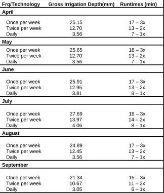
Table 2.2 Gross irrigation depth (mm) and runtime settings (minutes) for the Acclima add-on and time-based irrigation systems.
Frq/Technology Gross Irrigation Depth(mm) Runtimes (min) April
Once per week 25.15 17 – 3x Twice per week 12.70 13 – 2x Daily 3.56 7 – 1x May
Once per week 25.65 18 – 3x Twice per week 12.70 13 – 2x Daily 3.56 7 – 1x June
Once per week 25.91 17 – 3x Twice per week 12.95 13 – 2x Daily 3.81 8 – 1x July
Once per week 27.69 19 – 3x Twice per week 13.97 14 – 2x Daily 4.06 8 – 1x August
Once per week 24.89 17 – 3x Twice per week 12.45 13 – 2x Daily 3.56 7 – 1x September
Figure 2.1 Soil-water plot to determine field capacity. Continuous lines represent water-content from monitoring sensors buried in all ten plots of one replication
Figur
Figure 2
re 2.5 Acclima
2.6 Acclima CS
a RS 500 modu
S3500 water o
ule with senso
on-demand sys or
Figure 2.7 Intellisense TIS240 ET controller
Figure 2.12 Shelter housing the controllers, transformer, relays and datalogger
Figure 2.14 Watchdog model 700 weather station
CHAPTER 3
3. Results and Discussion
3.1 Sprinkler Uniformity Testing
Sprinkler uniformity testing was done to measure the distribution of applied water
over the plot area. The uniformity testing conducted prior to the experimental period on
18 April resulted in a wide range of both DU and CU values. The DU ranged from 25.1%
to 83.5% with an average of 69% while CU ranged between 56.5% and 90.7% with an
average of 81% (Table 3.1). The low value of 25.1% was due to a malfunctioning
sprinkler head that was subsequently replaced. Only one of the forty plots (replicate1 -
plot1) was not tested for irrigation uniformity because of a faulty sprinkler head that
required a replacement. Cardenas-Lailhacar et al. (2005) found a CU average of 71%
with a range of 50% to 89% and an average DU of 52% with a range of 15% to 78% for
the same type of sprinkler irrigation system in a similar study conducted in Florida. They
reported that the low value of DU (15%) in their study was because of a broken sprinkler
head which was replaced after testing.
Table 3.2 gives the values of DU and CU of uniformity testing performed on
October 16th (2007). Sprinkler uniformity decreased by 17% for DU and 8% for CU with
the DU values between 27.1% and 73.2% with an average of 55.4% and CU values
between 59.2% and 84.8% with an average of 73.4%. The possible reasons for the
decrease in the uniformity coefficients were clogged sprinkler head filters and wind drift
3.2 Evaluation of the Control Technologies
The study period in 2007 was warmer and drier than average. The 30-year (1971
– 2000) normal maximum temperature was 29.6ºC while the average maximum
temperature for the 20-week period was 30.8ºC (see Figure 3.1). Also the cumulative
rainfall for the same 30-year period was 540 mm while the cumulative rainfall for the
study period was 290 mm with 79 mm falling on the 19th July (see Figure 3.2). A plot of
the rainfall and cumulative rainfall that occurred during the experimental period is shown
in Figure 3.3. Pump failures occurred during the course of the study preventing possible
scheduled irrigations on a total of six days. This impacted the once per week irrigation
frequencies more severely, as the next available irrigation was delayed by seven days.
While the pressure regulators were set for 207 kPa, cycles of de-pressurization and
re-pressurization during pump failures or filter cleaning altered the pressure settings. In
general replications three and four were pressurized slightly higher after these instances
and received more water than replications one and two until the regulators were manually
reset. Total applied water for all the technologies and frequencies is given in Table 3.4.
3.2.1 Standard time-based system
Total gross irrigation amounts applied for the time-based system were; once per
week – 429 mm, twice per week – 430 mm, and daily – 395 mm. The values for the
cumulative irrigation were similar for the three frequencies as they were programmed to
apply the same irrigation amounts weekly and only differed in the setting of rain sensor
twice per week treatments because of a higher proportion of skipped irrigations. No
irrigation was applied on 28 out of a possible 140 occasions (22 due to the rain sensor
override and 6 due to pump failures) while the once per week treatment did not irrigate
on 3 out of a possible 20 occasions and the twice per week treatment did not irrigate on 6
out of a possible 40 occasions due to rain sensor override.
Comparison of the cumulative net irrigation water applied for each frequency to
the cumulative estimated crop evapotranspiration (ETc, using Penman-Montieth
generated reference ET from the weather station and a crop coefficient of 0.8) over the
experimental period is shown in Figure 3.4. The cumulative ETc for the entire period was
508 mm while the cumulative net irrigation (gross irrigation x CU) for the three
frequencies were; once per week – 343 mm, twice per week – 344 mm, and daily – 316
mm. The volumetric soil water content, irrigation and rainfall depths for the three
frequencies are shown in Figures 3.5 - 3.7.
3.2.2 Acclima add-on system
The Acclima add-on system was programmed with an irrigation schedule
identical to the based system but applied 18% to 48% less water than the
timer-based system. This was due to the volumetric soil water content being above the setpoint
on several occasions when irrigation was scheduled. The cumulative gross irrigation
amounts were: once per week – 219 mm, twice per week – 325 mm, and daily – 347 mm.
The once per week treatment skipped irrigation on 8 occasions and twice per week
daily treatment compared to the time-based technology was mainly because of a higher
number of skipped irrigation opportunities. The daily irrigation treatment skipped 40
potential irrigations (34 due to sensor override and 6 due to pump failures).
Comparison of the cumulative net irrigation water applied for each of the
frequencies to the cumulative estimated ETc is shown in Figure 3.8. The total net
irrigation amounts were: once per week – 175 mm, twice per week – 260 mm and daily –
278 mm. The volumetric water content, rainfall and irrigation depths for the three
frequencies are given in Figures 3.9 – 3.11. Figure 3.11 shows that the soil water content
was high even though no rainfall occurred between 25th July and 6th of August. This
might have occurred because of possible internal drainage and preferential flow of water
from rainfall and irrigation from adjacent plots. It was also observed that the neighboring
plot (timer-based daily treatment) had a similar spike during the same period.
There have been other studies that evaluated similar add-on type systems.
Cardenas-Lailhacar et al (2005) found water savings of 59% to 88% compared to a
timer-based system using the same technology in a study conducted in Florida. This is because
of the frequency and amount of rainfall during the study that experienced two hurricanes
and high rainfall (nearly 950 mm). As a result there were more skipped irrigation events.
Even though this research had water savings, there was significant stress in turf towards
the end of the experimental period again as a result of dry weather. Dukes and Scholberg
(2004) observed 23% and 50% water savings using TDR probes and a dielectric sensor
compared to a conventional irrigation system. Although water savings of this system was
comparable with other research, the system as a whole fell behind in terms of turf quality
especially at the end of the study because of the drought conditions that prevailed the
entire summer.
3.2.3 Acclima water on-demand system
The total gross irrigation for the 20-week study period was 448 mm or 7% more
water than the timer-based system. The Acclima CS3500 system failed twice during the
experimental study, once on the 14th of May and again on the 12th of June, perhaps due
to lightning at the field site. No soil-water data were collected by the monitoring
(continuous) sensors for any of the treatments from 14-18 May and 12-18 June and no
irrigation occurred for the on-demand technology during these periods. These failures did
not affect the total applied water by the system as replacement units were installed prior
to the soil-water level falling below the turn-on setpoint. The volumetric soil-water
content, irrigation and rainfall events are plotted in Figure 3.12 and it can be observed
that the system tried to maintain the soil-water level between the two setpoints
throughout the experimental period. The cumulative net irrigation for this technology was
358 mm, and comparison with cumulative estimated ETc is shown in Figure 3.8.
3.2.4 ET controller system
The volumetric water content, irrigation and rainfall events plots for the three
frequencies are given in Figures 3.13 - 3.15. The total gross irrigation amounts were;