Dynamical systems modeling to identify a cohort of problem drinkers with similar mechanisms of behavior change

(1)

Dynamical systems modeling to identify a cohort of problem

drinkers with similar mechanisms of behavior change

Kidist Bekele-Maxwell *a, R. A. Everett *a, Sijing Shao *c, Alexis Kuerbis b, Lyric Stephensona_{, H. T. Banks}a_{, and Jon Morgenstern}c

a_{Center for Research in Scientific Computation, North Carolina State University} b_{Hunter College, City University of New York}

c_{Northwell Health}

*_{These authors contributed equally}

(2)

Abstract

One challenge to understanding mechanisms of behavior change (MOBC) completely among

individuals with alcohol use disorder is that processes of change are theorized to be complex,

dynamic (time varying), and at times non-linear, and they interact with each other to influence

alcohol consumption. We used dynamical systems modeling to better understand MOBC within

a cohort of problem drinkers undergoing treatment. We fit a mathematical model to ecological

momentary assessment data from individual patients who successfully reduced their drinking by

the end of the treatment. The model solutions agreed with the trend of the data reasonably well,

suggesting the cohort patients have similar MOBC. This work demonstrates using a personalized

approach to psychological research, which complements standard statistical approaches that are

often applied at the population level.

Key words: Mathematical psychology, inverse problems, behavior change, personalized medicine,

(3)

Introduction

Recently, the National Institute of Health proposed precision medicine as a means to improve the

efficiency and effectiveness of treatments of all disease (Centers for Disease Control and Prevention,

2016). The primary principle of precision medicine is that one aims to identify the unique

com-ponents of both health and disease of each individual so that an extremely tailored and targeted

intervention or set of interventions can be provided to the individual to maximize their efficacy.

Where previously medicine pursued a one size fits all treatment, or the treatment that was most

effective for the most people, emphases have now been placed on an individually tailored approach

in order to advance healthcare to its next generation. In taking such a perspective, the focus of

research must shift to include how individuals differ from group averages.

One disease to which precision medicine can be applied is alcohol use disorder (AUD).

Ex-cessive alcohol consumption is known to cause the deaths of about 88,000 people each year in the

United States and is associated with an estimated public health cost of about$249 billion in 2010

(Centers for Disease Control and Prevention, 2016). While a number of treatment interventions

are available for AUD, treatments remain only modestly effective (Longabaugh et al., 2013). In

order to improve interventions for individuals with AUD, mechanisms of behavior change (MOBC)

both for treatment related and self-initiated drinking reduction need to be understood (Huebner

& Tonigan, 2007). Identifying MOBC can help healthcare providers implement more efficient and

effective interventions by understanding the crucial factors that initiate and maintain the change

process.

A critical challenge to obtaining a more complete understanding of MOBC among individuals

with AUD is that processes of change are theorized to be complex, dynamic (time varying), and

(4)

Such complexity presents challenges to both data collection and data analyses. One way to better

understand these change processes is by collecting data on individuals as they interact with their

natural environment in real time. Extensive, real time data collection can occur inexpensively,

efficiently, and accurately using ecological momentary assessment (EMA), which is designed to

collect ecologically valid data about behavior, thoughts, and feelings over time, while avoiding the

pitfalls of retrospective recall (Shiffman, 2009).

In conjunction with EMA, mathematical modeling can be utilized to understand these

com-plex, highly interactive, time varying, and non-linear data. While advanced statistical procedures

can be used effectively with intensive, longitudinal datasets (e.g., Boker & Laurenceau, 2006), such

statistical procedures tend to reduce results to averages across individuals, thereby limiting the

amount of information that might be gleaned from a particular dataset. Mathematical modeling

provides an exciting compliment to such methods by modeling time varying relationships between

variables and nonlinear systems represented by repeated measurement data (Davidian & Giltinan,

1995).

Mathematical modeling has already been used as a method of understanding social behaviors.

Since cyclic patterns are a fundamental element of many psychological theories (Chow et al., 2009),

mathematical oscillator models have been utilized to help improve the understanding of these

processes. For example, oscillation models have been used to describe the dynamics of several

psychological constructs, such as emotion, stress and affect, and intimacy (Chow et al., 2005;

Bisconti et al., 2004; Montpetit et al., 2010; Boker & Laurenceau, 2006). Mathematical modeling

efforts in the context of alcohol consumption have been mainly implemented at the population level.

For example, previous efforts applied mathematical epidemiology techniques to reflect

(5)

Previously, a dynamical systems modeling approach was initiated to understand the changes in

drinking behaviors at a personal level (Banks, Rehm, et al., 2014). In this study, the authors

inves-tigated several key factors related to MOBC among individuals with AUD. In a subsequent study

(Banks, Bekele-Maxwell, et al., 2016), the authors then applied this new approach to build a

pre-liminary model of behavior change. They relied on theories of behavior change related to substance

abuse in developing the model and selecting four primary variables that vary over time.

In the present work, we extended this modeling effort. We first identified a cohort of

par-ticipants from a sample of problem drinkers recruited into a randomized controlled trial of brief

treatment for AUD called Project SMART (Morgenstern et al., 2012). The participants selected

for this cohort successfully reduced their drinking during treatment and were hypothesized to share

the same underlying MOBC in alcohol consumption. We then developed and honed a

mathe-matical model using each of their data during the iterative process of modeling to determine the

relationships between the identified variables.

Data Collection

Project SMART was a study that tested the combined effectiveness of modified behavioral

self-control therapy (MBSCT) and naltrexone (NTX) in problem drinking men who have sex with men

(MSM) (Morgenstern et al., 2012).

Method

Participants.

Participants responded to online and print advertisements targeting MSM who wished to

(6)

standard drinks per week; identify as sexually active with other men over the preceding 90 days; and

read English at an eighth grade level or higher. Participants were excluded if they: 1) had a lifetime

diagnosis of bipolar disorder, schizophrenia, or other psychotic disorders; 2) an untreated current

major depressive disorder; or 3) current physiological dependence on alcohol or other drugs (with

the exception of nicotine or cannabis), as demonstrated by current physical withdrawal symptoms

or a history of severe withdrawal syndrome; 4) started or changed psychotropic medication in the

preceding 90 days; 5) were at risk for serious medication side effects from naltrexone; 6) reported

regular use of opioids; or 7) were enrolled in concurrent drug- or alcohol-related treatment during

the 12-week treatment phase of the study (Morgenstern, et al., 2012). The typical participant was

male, approximately 40 years old, Caucasian, attended at least some college, and employed.

Procedures.

After initial screening, eligible and enrolled participants (N = 200) were randomized to one

of four conditions: placebo only (PBO), naltrexone only (NTX), Modified Behavioral Self-Control

Therapy only (MBSCT), or both naltrexone and MBSCT (NTX + MBSCT). At the end of 12

weeks of treatment, all participants received a follow-up assessment.

Study Interventions. All participants received Brief Behavioral Compliance Enhancement

Treatment (BBCET), a series of 20-minute sessions with a psychiatrist weekly for the first three

weeks, and then every other week thereafter. Participants were blind to medication condition.

Dosage of naltrexone was initiated at 25 mg/day, and then increased to 100 mg/day during the

first three weeks of treatment. For those who received MBSCT, treatment was a combination

of motivational interviewing and cognitive behavioral therapy and comprised of 12 one-hour

psy-chotherapy sessions that focused on moderation as a goal.

(7)

telephone survey delivered via Interactive Voice Recording (IVR) (TELESAGE, 2005) between 4:00

pm and 10:00 pm each day, for a total of 84 days. The questionnaire consisted of 30-45 questions

and collected information related to emotions, daily events, and drinking behaviors. Participants

received an automated reminder call if they failed to call into the system by 8:00 pm. Each survey

required between 2 to 5 minutes to complete.

Measures.

All four measures used in this study were from EMA.

Daily alcohol consumption.

Alcohol consumption was assessed by having participants report the number of standard drinks of

beer, wine, and liquor consumed in the past 24 hours.

Norm violation.

Norm Violation was assessed by asking, Do you consider the total amount you have had to drink

since this time yesterday to be excessive? That is, was it more than you think you should have had?

The response set ranged from 0 (Definitely Not) to 3 (Definitely).

Personal norm. The thresholds (i.e., norms) individuals used to evaluate whether or

not their drinking was excessive is referred to here as “personal norm”. Personal norms vary across

individuals and can be considered to be dynamic across time and setting of drinking. Personal

norm in this study is a latent variable and thus was not directly measured. We include this latent

variable in our modeling process.

Confidence.

Confidence was measured by asking, How confident are you that you can resist drinking heavily

(that is, resist drinking more than 5 standard drinks) over the next 24 hours? The response set

(8)

Commitment.

Commitment was measured by asking,How committed are you not to drink heavily (that is, not to

drink more than 5 standard drinks) over the next 24 hours? The response set ranged from 0 (Not

at all) to 4 (Extremely).

Analytic Plan

Variable selection.

Based on findings from previous studies (Morgenstern et al., 2016; Kuerbis et al., 2014), a dual

process theoretical framework for substance abuse (Morgenstern et al., 2013) was utilized 1) to select

four key variables that directly relate to the number of drinks consumed, and 2) to try to understand

how those variables interact with each other over time. The dual process framework for addiction

proposes a top-down, bottom-up cognitive process in which top-down executive functioning (e.g.,

commitment not to drink) attempts to control responses to stimuli (e.g., alcohol) which also evoke

implicit cognitive processes. The variables identified to represent the dual process model were:

alcohol consumption, norm violation, confidence, and commitment. While desire was included as

a constant factor in the model, it was excluded as a variable of focus from this initial iterative

model building process. Further exploration of desire will occur during a future stage of model

development.

Mathematical modeling methodology and participant selection.

Mathematical models can represent and describe psychological processes using mathematical

ex-pressions. The dynamical modeling approach used here to examine MOBC is an iterative process

(Figure 1). In general, a preliminary mathematical model is proposed based on existing

(9)

how accurately the model describes the underlying psychological process. This evaluation should

either confirm existing psychological theories or lead to a new psychological understanding of the

relationships among the variables. The latter can then lead to model adjustment and a repeated

cycle. The mathematical model quantifies how the key variables change over time and how they

interact among each other.

The psychological process described by the mathematical model depends on parameters, which

are often unknown or not directly measurable. These unknown parameters are often estimated by

solving an inverse problem, which is, given an individual’s dataset and mathematical model, the

problem of estimating parameters that would generate such a dataset. The resulting parameters

should minimize the distance between the model solution and the data. The model solution is

personalized for that individual according to the particular set of parameters.

Before solving an inverse problem, the correct statistical error model needs to be identified

in order to account for the uncertainty in the data (observation error). Misspecifying the error

structure can lead to an incorrect estimation of the parameters (Banks, Hu, & Thompson, 2014;

Banks & Tran, 2009). If the error does not depend on the size of the observations (i.e., the error is

evenly distributed across various observation sizes), an ordinary least squares method is appropriate

for parameter estimation; if, however, the error depends on the size of the observation (i.e., the

error does not remain constant over observation sizes), an Iterative Weighted Least Squares (IWLS)

method is required.

To account for the uncertainty in the data, let Yi,j be a random variable associated with

(10)

model

Y1,j=f1(tj;θθθ0) +f1(tj;θθθ0)γ1E1,j

.. .

Y4,j=f4(tj;θθθ0) +f4(tj;θθθ0)γ4E4,j,

wheref1(tj;θθθ0), . . . , f4(tj;θθθ0) represent the mathematical model solution for variables alcohol

con-sumption, norm violation, confidence, and commitment, respectively (see the mathematical model

below) at time j with the nominal parameter vector θθθ0, which is assumed to exist. The term

fi(tj;θθθ0)γiEi,j represents the measurement error that causes the data to not exactly equalfi(tj;θθθ0).

We assume the random vector E_j = (E₁_,j, . . . ,E₄_,j)T are independent and identically distributed

(i.i.d) with mean zero. We represent the obtained data, yi,j, collected at time j for variable i, for

j= 1, . . . , nby the following

y1,j=f1(tj;θθθ0) +f1(tj;θθθ0)γ11,j

.. .

y4,j=f4(tj;θθθ0) +f4(tj;θθθ0)γ44,j,

wherei,j is a realization of the random variableEi,j. See Banks, Bekele-Maxwell, et al. (2016) for

further details on the statistical error model and implementation of the IWLS method.

In Banks, Bekele-Maxwell, et al. (2016), the mathematical model was developed using one

participant’s data. In this study, we continue the iterative modeling process by both slightly

improving the mathematical model and by applying this model to three additional patients who

reduced their drinking. We fit the mathematical model to each of them and determined they shared

a common set of mechanisms. These patients were then identified as a cohort.

(11)

formulated the mathematical model. For each patient’s dataset, we then determined the correct

statistical error model using asecond-order differencing methodto quantify the observation error for

alcohol consumption, norm violation, confidence, and commitment (Banks, Catenacci, & Hu, 2016).

The results revealed that the IWLS method was appropriate in our case with γγγ = [γ1, γ2, γ3, γ4],

whereγ1,γ2, γ3, and γ4 correspond to alcohol consumption, norm violation, confidence, and

com-mitment respectively for each individual patient. We finally solved the inverse problem to estimate

the patient-specific mathematical model parameters and compare the model solution to each

pa-tient’s dataset.

Mathematical Model

Here we present the mathematical model from Banks, Bekele-Maxwell, et al. (2016) with a

modifi-cation that better quantifies the trend of commitment in the selected patients. A schematic (Figure

2) representing the relationships among the variables is created based on prior psychological

knowl-edge and observations of the data.

Timing of variables. The variableA(t) represents daily alcohol consumption, or the number

of alcoholic drinks a person has consumed in the past 24 hours from time t(i.e., from timet−1 to

timet). V(t) represents norm violation on a particular day (timet). Norm violation also relates to

the period between t−1 and t. Cf(t) represents the confidence level a person feels at timet that

he can resist drinking heavily in the next 24 hours (i.e. from timetto timet+ 1). Ch(t) represents

the commitment a person makes to not drink heavily in the next 24 hours at timet(i.e. from time

tto time t+ 1).

Schematic model to mathematical model. The model is built by formulating

(12)

schematic diagram corresponds to a term in the model (Banks, Bekele-Maxwell, et al., 2016). For

example, arrow 2 in Figure 2 corresponds to term 2 in Equation (1a) such that if the participant

feels that his drinking in the past 24 hours violated his personal norm, his drinking will decrease

in the next 24 hours.

The mathematical model is given by the following

dA

dt =|{z}a1

1

−a2V(t−1)

| {z }

2

−a3Ch(t−1)

| {z }

3

−a4Cf(t−1)Ch(t−1)

| {z }

4

(1a)

dV

dt =χ(A>A∗)v1

d(A−A∗)

dt

| {z }

5a

−χ₍_A≤A∗₎v₂V

| {z }

5b

(1b)

dCf

dt = −χ(A>5)d1 dA

dt Ch(t−1)

| {z }

6a

+χ(A≤5)d2(Cf−α)

1−Cf

n

| {z }

6b

, (1c)

dCh

dt =mCh

1−Ch

K

| {z }

7

(1d)

where

A∗(t) =be−rt+l

| {z }

8

, (1e)

and

χA>A∗ =

          

1 ifA > A∗

0 else

, χA≤A∗ =

          

1 ifA≤A∗

0 else

. (1f)

The equations above include the hypothesized MOBC based on theories of behavior change

and our previous studies. For this particular model, we assume desire to be constant.

Individual equations. In Equation (1a), term 1 describes how the rate of change of alcohol

consumption is increased by one’s desire to drink, which is held constant here. Terms 2 and 3

(13)

24 hours to be excessive, and if he is committed to not drink heavily, respectively. In addition, if

the participant feels both confident and committed that he can resist drinking heavily in the next

24 hours, then his alcohol consumption decreases. However, if the participant feels confident but

definitely not committed, then his confidence level will not affect his alcohol consumption (term

4).

Equation (1b) describes how the rate of change in norm violation depends on the patient’s

alcohol consumption relative to his personal norm, A∗. If the participant drank less than or equal

to his personal norm in the past 24 hours, his norm violation will decrease exponentially to 0 (term

5b). If the participant drank more than his personal norm in the past 24 hours, the change in norm

violation is dependent on the rate at which the number of drinks approaches the personal norm,

denoted by d(A−_dtA∗) (term 5a). His norm violation decreases if his alcohol consumption decreases

towards his personal norm at a faster rate than the rate of decrease in his personal norm. His norm

violation increases if his alcohol consumption decreases at a slower rate compared to his personal

norm or if his alcohol consumption increases away from his personal norm.

Equation (1c) describes that the rate of change in confidence depends on whether the patient

is drinking heavily or not (recall drinking heavily is five alcoholic drinks or more, according to

NIAAA):

1. If the participant drinks heavily (more than 5 drinks in last 24 hours) and he feels

commit-ted, his confidence depends on the rate of alcohol consumption, dA_dt; if the patient’s alcohol

consumption is increasing (decreasing) over time, then his confidence will decrease (increase).

2. In addition, if the participant drinks less than 5 drinks in 24 hours, then his confidence

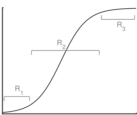
will increase logistically (Figure 3). The logistic model is well established and often used in

(14)

the participant first stops drinking heavily (R1, bottom of the curve), he will need to establish

a habit of drinking lightly for a few days. As he gains a sense of mastery, his confidence will

increase more quickly towards his maximum confidence level (R2, steep, middle of the curve).

After the participant has mastered this habit of drinking lightly, his increase in confidence

slows as he “reaches” his maximum confidence level (R3, top of the curve).

Equation (1d) captures the hypothesis that a participant’s motivation level (i.e., commitment)

increases as the treatment period progresses. We quantify this increase using a logistic model rather

than the previous function presented in (Banks, Bekele-Maxwell, et al., 2016) to allow for a slower

increase in commitment at the beginning of treatment.

Equation (1e) describes that the personal norm decreases during the treatment period.

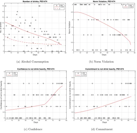
Model Solutions Describing MOBC

Below we present the results for four participants (condition noted in parentheses), 1761 (MBSCT),

1771 (MBSCT), 1474 (NTX + MBSCT) and 1460 (NTX). As we can see in Figures 4 - 7, the model

describes the relationships among the variables reasonably well. The data in the figures are averaged

weekly IVR data. As it will be described below, we use these averaged data to better show the

overall trend of the data; we use patient 1474 to illustrate that as we average over 3, 5, and 7 days,

it becomes more obvious that the trend in the data is captured by the model. Similar results can

be found for all four patients in the supplemental material section. We then discuss the results for

(15)

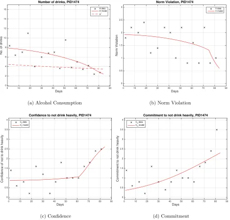
Rationale of Using Average vs. Daily Data

As mentioned above, the model solutions presented for the four patients are fit to the IVR data

averaged weekly in order to better show the trend of the data over the course of the treatment

period. Initially, we fit the model to the daily IVR data. However, we were interested in modeling

the general trend of the data rather than the daily fluctuations. Due to the nature of the data

(qualitative or Likert type data (Likert, 1932)), we found that it is difficult to determine if the

continuous model solutions follow the dynamics in the data on a fine scale. Therefore, we averaged

the data over 3, 5, and 7 days and fit the model to these modified datasets.

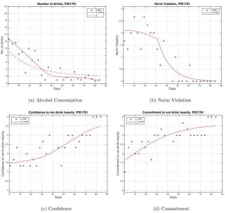
To illustrate how averaging can better show the overall trend in the data, we present the results

for a sample patient (PID 1474). Figures 8 - 10 and 6 contain the original data, and data averaged

over 3, 5, and 7 days, respectively for this sample patient. Note that ‘o’ represents the daily data

while ‘x’ represents the averaged data. Each figure also contains the corresponding model solution

for that dataset. Notice that as more data is averaged, the trend in the data and the agreement

with model solutions becomes more apparent. For example, the data in Figure 8c looks scattered

and it is not obvious that the model solution represents the overall confidence dynamics. Even

though the model solution is visually similar for each dataset (Figures 9c, 10c, 6c), as the data is

averaged over longer time periods, it becomes progressively evident that the model is describing

the underlying MOBC reasonably well. A similar pattern can be observed for number of drinks,

norm violation, and commitment.

Cohort Results

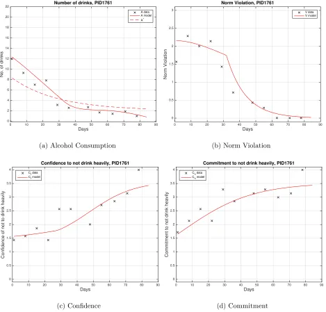
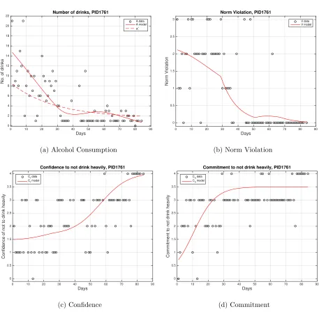
PID 1761. In Figure 4a, we can see that this patient reduces his drinking to a moderate

(16)

the treatment period, which is captured by the model solution (solid red line). The data show

that there is a significant behavior change occurring between days 20 and 30 in treatment. This

behavior is represented by the model solution, which indicates after approximately day 30, 1761

starts drinking less than his personal norm (dashed red line), and remains below this level for the

rest of the treatment period.

In Figure 4b, 1761’s norm violation data is often above an average value of 2 (Probably) in

the first month and then decreases quickly towards 0 (Definitely Not) for the remainder of the

treatment period. This behavior is captured by our model solution.

In Figures 4c and 4d, the data and model solution show that there is an increase in both

confi-dence and commitment as the patient decreases his drinking level. The patient starts the treatment

period with a confidence and commitment level of approximately 1.5 (Somewhat -Moderately) and

then increases towards the maximum level of 4 (Extremely). Notice that in Figure 4c, the patient’s

confidence initially increases slowly until around day 30, at which point he stops drinking heavily.

His confidence then increases rapidly after he has mastered the habit of drinking moderately.

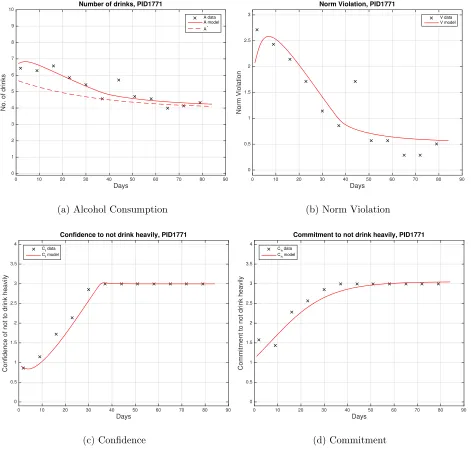
PID 1771. In Figure 5a, we can see that the patient successfully reduced his drinking

from a heavy to a more moderate level (average 6.5 to 4.2 drinks per day). The model solution

in Figure 5a expresses the overall reduction in number of drinks during the treatment period.

Although the patient’s alcohol consumption decreases towards his personal norm, he never achieves

this threshold. Note that the patient returns to drinking heavily around day 45. However, around

this time the patient’s confidence and commitment remain at his highest level, indicating that some

other factor causes this high drinking. Thus our model solution does not reflect this.

In Figure 5b, the norm violation data and model solution decrease from a high level (Probably

(17)

not ever reach an averaged value of 0 (Definitely Not), but remains around 0.5 towards the end of

the treatment period. This is indicated by the fact that his alcohol consumption stays above his

personal norm in Figure 5a. We note that the patient has a higher norm violation around day 45

due to the heavy drinking around the same time.

In Figures 5c and 5d, the patient’s confidence and commitment increase from approximately

a level of 1 (Somewhat) to a level of 3 (Very) within the first month, and then remain at this level

for the rest of the treatment period, as represented by both the data and model solutions.

Overall, this patient stops drinking heavily about a month into treatment. After this point,

all four variables remain somewhat constant, indicating that he is most likely satisfied with his

drinking habit (Not Drinking Heavily).

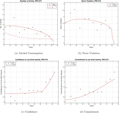
PID 1474. In Figure 6a we can see that, even though the data is a little sporadic, the

trend of the patient’s alcohol consumption decreases from heavy drinking to below an average of

4 drinks per day towards the end of the treatment period. The model solution follows a similar

pattern. It also indicates that the patient reaches his personal norm around day 80, which is

reasonable because his norm violation goes to an average value of 0 around the same day (Figure

6b).

Again, although the patient’s norm violation data is a bit scattered (Figure 6b), overall we

see a decrease over the treatment period. This decrease in norm violation is significant around day

80, which the model solution also agrees with.

In Figure 6c, the data shows that the patient’s confidence remains low until around day 65, at

which point it increases to 3 (Very Confident). This is reflected in the model solution, as confidence

starts to increase immediately after the patient stops drinking heavily around day 65. Similarly,

(18)

6d).

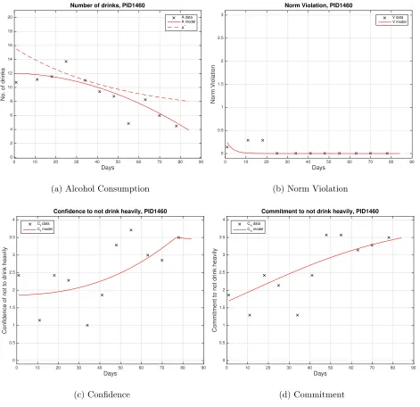
PID 1460. In Figure 7a, the patient starts the treatment period drinking heavily and

then reduces his drinking on average to just below the heavy drinking threshold. These dynamics

are well captured by the model solution. We note that this patient remains below his personal norm

over the course of the treatment period, which explains why his norm violation data and solution

decreases quickly to zero and remain there (Figure 7b). This suggests that norm violation is not

as significant as confidence and commitment in reducing the patient’s alcohol consumption.

In Figures 7c and 7d, we can see that although the confidence and commitment data are

dispersed, the model solutions are able to exhibit the general increasing trend.

Discussion

This study used mathematical modeling as a complementary method to standard statistical

ap-proaches to help understand the dynamic process of behavior change in the context of alcohol use

disorder. It demonstrates how mathematical modeling can be a tool to examine mechanisms

under-lying drinking reduction with a focus at the individual level, and in doing so, nuanced relationships

between variables can be identified that might not have otherwise been determined through

tradi-tional statistical methods. By building upon the work by Banks, Bekele-Maxwell, et al. (2016), this

study extended the iterative effort of improving the original model by applying the model to three

additional “treatment responders”—individuals who dramatically reduced their drinking during

the study period and had more complete data. We fit the mathematical model to each patient’s

data to determine whether a common set of mechanisms emerged, such that the decrease in their

alcohol consumption was explained by norm violation, confidence, and commitment. Through this

(19)

equation for behavior change emerged. Thus, we demonstrated the ability to iteratively move from

a single-case model to a cohort with similar underlying MOBC. Next steps will include testing the

model with other treatment responders that have less complete data to see if the model continues

to hold across participants.

Some interesting findings result from this model building process. Alcohol consumption, norm

violation, confidence and commitment in the model are allowed to increase or decrease at varying

speeds allowing for each individual to demonstrate a unique speed and process of change.

Further-more, unlike previous traditional statistical work we have performed (e.g., Morgenstern et al., 2016),

this model identified an important combined effect of commitment and confidence—confidence can

be high, but without commitment, drinking does not decrease. In addition, while norm violation

has been a construct of focus in studies on personalized feedback (Carey et al., 2010; Larimer et al.,

2009), it has been less of a focus in the context of ongoing treatment. In collecting and evaluating

daily data on whether a person evaluated their drinking as excessive, we identified a latent dynamic

construct—one’s personal definition of normative drinking—as being particularly important in

in-fluencing potential successful reduction in drinking in a more intensive treatment protocol, beyond

feedback about drinking. Our modeling efforts suggest collecting information about a person’s

personal norm threshold would be an important area of future research.

Study Limitations

Given the developmental nature of this work, there are several study limitations to consider. Even

though recent studies (Morgenstern et al., 2016; Kuerbis et al., 2014) were utilized to help us

understand how the key variables interact with each other over time, the modeling process is

(20)

behavior change in patients with AUD that include non-linear relationships. In addition, this study

employed a secondary data analysis design where data were not collected for modeling purposes.

Thus, the inability to identify a strong linear trend using daily data may reflect limitations in

the data collection. For example, confidence, commitment, and norm violation were measured

as discrete ordinal variables, whereas they are generally modeled as continuous variables since a

patient probably feels a continuous change instead of a sudden jump from one level to another.

New data is currently being collected that includes more response options to improve the quality of

data in preparation for a next round of modeling. Furthermore, we utilized visual inspection and

analysis of alcohol consumption to determine which participants to include in the iterative model

development process, which inherently impacts the model results. This method also does not allow

for generalizability to a larger group until the model has been tested for fit across a larger group

of participants. The next step in our research will be to see if the model successfully applies to a

wider group of problem drinkers who respond to treatment and have less complete data. Given the

sample used in this study, potential mechanisms identified here can only initially be considered to

apply to problem drinking MSM rather than a wider population of problem drinkers.

Conclusion

Increasingly, behavior change is being seen as a complex, dynamic phenomena that operates at an

individual level (Riley et al., 2011). For example, social learning theories that underlie most AUD

behavioral interventions posit the individual level therapy outcomes are the results of interactions

between traits, dynamic internal factors, contexts, treatments, and time. The nature of these

interactions including the time frames for how variables (slow-moving versus fast acting) effect

these interactions is as yet unknown. Attempting to use methods (e.g., modeling on the

(21)

clarify the nature of these interactions. Standard linear approaches, including multi-level modeling,

are limited in handling complex interactions, such as nonlinear relationships and feedback loops,

and especially those involving time (Tan et al., 2012). Mathematical modeling provides a useful

complimentary and supplementary approach to these standard methods as a way of identifying

nuanced relationships between variables and for providing more information about future areas of

exploration for MOBC research, including data collection procedures, new constructs of focus, and

(22)

Figures

(1)

Experiments and data collection

(Empirical observations)

(2)

Psychological model

(Formalization of psychological relationships, properties, and mechanisms)

(3)

Mathematical model

(Abstraction of psychological process)

(4)

Statistical error model

(Formalization of uncertainty / variability in data)

(7)

Changes in understanding of psychological process

The Iterative

Modeling Process

(6)

Interpretation and comparison to the real psychological system

(5)

Model analysis

(Numerical and/or analytical)

Figure 1: The Iterative Modeling Process (Banks & Tran, 2009). The white boxes indicate steps

(23)

C

f

(t)

A(t)

V(t)

C

h

(t)

Treatment/

Time

− + (A*, (A-A*)’)

+ − (A’,Ch>0)

2

5

4 3

6

7

Constant desire 1

−

− (Ch>0)

+

Figure 2: Schematic of hypothesized variable relationships (Banks, Bekele-Maxwell, et al., 2016).

A(t) represents alcohol consumption, A∗ represents the number of drinks that a person believes

to be his norm, V(t) represents norm violation, Cf(t) represents confidence, and Ch(t) represents

commitment. The arrows represent the hypothesized variable relationships.

R

1

R

2

R

3

(24)

Days

0 10 20 30 40 50 60 70 80 90

No. of drinks

0 2 4 6 8 10 12 14 16 18 20

22 Number of drinks, PID1761

A data A model A*

(a) Alcohol Consumption

Days

0 10 20 30 40 50 60 70 80 90

Norm Violation 0 0.5 1 1.5 2 2.5 3

Norm Violation, PID1761

V data V model

(b) Norm Violation

Days

0 10 20 30 40 50 60 70 80 90

Confidence of not to drink heavily

0 0.5 1 1.5 2 2.5 3 3.5 4

Confidence to not drink heavily, PID1761

Cf data C_f model

(c) Confidence

Days

0 10 20 30 40 50 60 70 80 90

Commitment to not drink heavily

0 0.5 1 1.5 2 2.5 3 3.5 4

Commitment to not drink heavily, PID1761

Ch data C_h model

(d) Commitment

Figure 4: PID 1761 weekly averaged data and model solution. Estimated parameter values are

a1 = 0.548, a2 = 0.286, a3 = 0.035, a4 = 0.043, v1 = 0.103, v2 = 0.085, d1 = 0.014, d2 = 0.114,

b = 6.479, r = 0.036, l = 2.063, m = 0.046, k = 3.520, A0 = 12.336, V0 = 2.159, Cf0 = 1.570,

(25)

Days

0 10 20 30 40 50 60 70 80 90

No. of drinks

0 1 2 3 4 5 6 7 8 9

A data A model A*

Days

0 10 20 30 40 50 60 70 80 90

Norm Violation 0 0.5 1 1.5 2 2.5 3

V data V model

(b) Norm Violation

Days

0 10 20 30 40 50 60 70 80 90

0 0.5 1 1.5 2 2.5 3 3.5 4

Cf data C_f model

(c) Confidence

Days

0 10 20 30 40 50 60 70 80 90

0 0.5 1 1.5 2 2.5 3 3.5 4

Ch data C_h model

(d) Commitment

a1 = 0.465, a2 = 0.155, a3 = 0.053, a4 = 0.024, v1 = 1.638, v2 = 0.141, d1 = 0.556, d2 = 0.245,

b = 1.769, r = 0.029, l = 3.946, m = 0.082, k = 3.052, A0 = 6.721, V0 = 2.075, Cf0 = 0.909,

(26)

Days

0 10 20 30 40 50 60 70 80 90

No. of drinks

0 2 4 6 8 10 12 14 16

Number of drinks, PID1474

A data A model A*

Days

0 10 20 30 40 50 60 70 80 90

Norm Violation 0 0.5 1 1.5 2 2.5 3

V data V model

(b) Norm Violation

Days

0 10 20 30 40 50 60 70 80 90

0 0.5 1 1.5 2 2.5 3 3.5 4

Cf data C_f model

(c) Confidence

Days

0 10 20 30 40 50 60 70 80 90

0 0.5 1 1.5 2 2.5 3 3.5 4

Ch data C_h model

(d) Commitment

a1 = 0.306, a2 = 0.168, a3 = 0.005, a4 = 0.077, v1 = 0.174, v2 = 0.561, d1 = 0.094, d2 = 0.144,

b = 2.818, r = 0.049, l = 2.123, m = 0.042, k = 3.483, A0 = 7.398, V0 = 1.537, Cf0 = 0.851,

(27)

Days

0 10 20 30 40 50 60 70 80 90

No. of drinks

0 2 4 6 8 10 12 14 16 18 20

A data A model A*

Days

0 10 20 30 40 50 60 70 80 90

Norm Violation 0 0.5 1 1.5 2 2.5 3

V data V model

(b) Norm Violation

Days

0 10 20 30 40 50 60 70 80 90

0 0.5 1 1.5 2 2.5 3 3.5 4

Cf data C_f model

(c) Confidence

Days

0 10 20 30 40 50 60 70 80 90

0 0.5 1 1.5 2 2.5 3 3.5 4

Ch data C_h model

(d) Commitment

a1 = 0.120, a2 = 0.000, a3 = 0.068, a4 = 0.005, v1 = 0.270, v2 = 0.325, d1 = 0.083, d2 = 0.224,

b = 9.443, r = 0.020, l = 6.212, m = 0.027, k = 3.998, A0 = 12.025, V0 = 0.238, Cf0 = 1.863,

(28)

Days

0 10 20 30 40 50 60 70 80 90

No. of drinks

0 2 4 6 8 10 12 14 16

A data A model A*

Days

0 10 20 30 40 50 60 70 80 90

Norm Violation 0 0.5 1 1.5 2 2.5 3

V data V model

(b) Norm Violation

Days

0 10 20 30 40 50 60 70 80 90

0 0.5 1 1.5 2 2.5 3 3.5 4

Cf data C_f model

(c) Confidence

Days

0 10 20 30 40 50 60 70 80 90

0 0.5 1 1.5 2 2.5 3 3.5 4

Ch data C_h model

(d) Commitment

Figure 8: PID 1474 data and model solution. Estimated parameter values are a1 = 0.336, a2 =

0.154,a3 = 0.092,a4= 0.041, v1= 0.381, v2 = 0.472,d1= 0.124, d2 = 0.134,b= 2.966, r= 0.043,

l = 2.357, m = 0.027, k = 3.154, A0 = 10.312, V0 = 2.490, Cf0 = 0.674, Ch0 = 0.432, α = 0.620,

(29)

Days

0 10 20 30 40 50 60 70 80 90

No. of drinks

0 2 4 6 8 10 12 14 16

A data A model A*

Days

0 10 20 30 40 50 60 70 80 90

Norm Violation 0 0.5 1 1.5 2 2.5 3

G data G model

(b) Norm Violation

Days

0 10 20 30 40 50 60 70 80 90

0 0.5 1 1.5 2 2.5 3 3.5 4

Conf data Conf model

(c) Confidence

Days

0 10 20 30 40 50 60 70 80 90

0 0.5 1 1.5 2 2.5 3 3.5 4

Ch data C_h model

(d) Commitment

Figure 9: PID 1474 data averaged every 3 days and model solution. Estimated parameter values

area1 = 0.898, a2 = 0.527, a3= 0.013, a4 = 0.145,v1 = 0.517, v2 = 0.031,d1 = 0.154,d2 = 0.212,

b = 4.629, r = 0.011, l = 2.450, m = 0.034, k = 4.221, A0 = 10.868, V0 = 3.194, Cf0 = 0.680,

(30)

Days

0 10 20 30 40 50 60 70 80 90

No. of drinks

0 2 4 6 8 10 12 14 16

A data A model A*

Days

0 10 20 30 40 50 60 70 80 90

Norm Violation 0 0.5 1 1.5 2 2.5 3

V data V model

(b) Norm Violation

Days

0 10 20 30 40 50 60 70 80 90

0 0.5 1 1.5 2 2.5 3 3.5 4

Cf data C_f model

(c) Confidence

Days

0 10 20 30 40 50 60 70 80 90

0 0.5 1 1.5 2 2.5 3 3.5 4

Ch data C_h model

(d) Commitment

area1 = 0.300, a2 = 0.150, a3= 0.064, a4 = 0.029,v1 = 0.179, v2 = 0.086,d1 = 0.070,d2 = 0.140,

b = 2.321, r = 0.006, l = 2.137, m = 0.031, k = 4.236, A0 = 7.871, V0 = 1.926, Cf0 = 0.878,

(31)

Acknowledgements

We would like to thank Judith Canner for her valuable insights and contributions. This research

was supported in part by the National Institute on Alcohol Abuse and Alcoholism under grant

number 1R01AA022714-01A1, in part by the Air Force Office of Scientific Research under grant

number AFOSR FA9550-15-1-0298, and in part by the National Science foundation under NSF

Undergraduate Biomathematics grant number DBI-1129214.

Author Contributions

Modified the original model and conceived the method to average the data: HB, KB, and RE.

Performed the computational work: KB, RE, SS, and LS. Wrote the first draft of the manuscript:

SS. Contributed to writing of manuscript: RE, KB, and AK. Made critical revisions and approved

final version: AK, HB, and JM. All authors reviewed and approved of the final manuscript.

Co-Investigators of Project SMART: JM and AK.

References

Banks, H. T. (1975). Modeling and control in the biomedical sciences (Vol. 6). Berlin:

Springer-Verlag.

Banks, H. T., Bekele-Maxwell, K., Everett, R., Stephenson, L., Shao, S., & Morgenstern, J. (2016).

Dynamic modeling of problem drinkers undergoing behavioral treatment. Bulletin of

(32)

Banks, H. T., Catenacci, J., & Hu, S. (2016). Use of difference-based methods to explore

statis-tical and mathemastatis-tical model discrepancy in inverse problems. Journal of Inverse and Ill-posed

Problems,24, 413-433.

Banks, H. T., Hu, S., & Thompson, W. C. (2014). Modeling and inverse problems in the presence

of uncertainty. Boca Raton: CRC Press.

Banks, H. T., Rehm, K. L., Sutton, K. L., Davis, C., Hail, L., Kuerbis, A., & Morgenstern, J.

(2014). Dynamic modeling of behavior change. Quarterly of Applied Mathematics,72, 209-251.

Banks, H. T., & Tran, H. T. (2009). Mathematical and experimental modeling of physical and

biological processes. Boca Raton: CRC Press.

Bisconti, T. L., Bergeman, C. S., & Boker, S. M. (2004). Emotional well-being in recently bereaved

widows: a dynamical systems approach. Journal of Gerontology: Psychological Sciences, 59B,

P158-P167.

Boker, S. M., & Laurenceau, J.-P. (2006). Dynamical systems modeling: an application to the

regulation of intimacy and disclosure in marriage. In T. A. Walls & J. L. Schafer (Eds.), Models

for intensive longitudinal data (p. 195-218). Oxford: Oxford University Press, Inc.

Carey, K. B., Henson, J. M., Carey, M. P., & Maisto, S. A. (2010). Perceived norms mediate effects

of a brief motivational intervention for sanctioned college drinkers. Clinical Psychology: Science

and Practice,17, 58-71.

Centers for Disease Control and Prevention. (2016). Alcohol use and your health. Retrieved from

http://www.cdc.gov/alcohol/fact-sheets/alcohol-use.htm

Chow, S. M., Hamaker, E. L., Fujita, F., & Boker, S. M. (2009). Representing time-varying

(33)

Statistical Psychology,62, 683–716.

Chow, S. M., Ram, N., Boker, S. M., Fujita, F., & Clore, G. (2005). Emotion as a thermostat:

representing emotion regulation using a damped oscillator model. Emotion,5, 208-225.

Davidian, M., & Giltinan, D. M. (1995).Nonlinear models for repeated measurement data (Vol. 62).

Boca Raton: Chapman & Hall/CRC.

Huebner, R. B., & Tonigan, J. S. (2007). The search for mechanisms of behavior change in

evidence-based behavioral treatments for alcohol use disorders: Overview. Alcoholism: Clinical

and Experimental Research,31, 1S-3S.

Kot, M. (2001). Elements of mathematical ecology. Cambridge: Cambridge University Press.

Kuerbis, A., Armeli, S., Muench, F., & Morgenstern, J. (2014). Profiles of confidence and

commit-ment to change as predictors of moderated drinking: A person-centered approach. Psychology of

Addictive Behaviors,28, 1065-1076. doi: 10.1037/a0036812

Larimer, M. E., Kaysen, D. L., Lee, C. M., Kilmer, J. R., Lewis, M. A., Dillworth, T., . . . Neighbors,

C. (2009). Evaluating level of specificity of normative referents in relation to personal drinking

behavior. Journal of Studies on Alcohol and Drugs, Supplement,16, 115-121.

Likert, R. (1932). A technique for the measurement of attitudes. Archives of Psychology,22, 5-55.

Longabaugh, R., Magill, M., Morgenstern, J., & Huebner, R. (2013). Mechanisms of behavior

change in treatment for alcohol and other drug use disorders. In B. S. McCrady & E. E. Epstein

(Eds.),Addictions: A comprehensive guidebook (2nd ed., p. 572-596). Oxford: Oxford University

Press.

Montpetit, M. A., Bergeman, C. S., Deboeck, P. R., Tiberio, S. S., & Boker, S. M. (2010).

(34)

Aging,25, 631-640.

Morgenstern, J., Kuerbis, A., Chen, A., Kahler, C. W., Bux, D. A., & Kranzler, H. (2012). A

randomized clinical trial of naltrexone and behavioral therapy for problem drinking

men-who-have-sex-with-men. Journal of Consulting and Clinical Psychology,80, 863–875.

Morgenstern, J., Kuerbis, A., Houser, J., Muench, F., Shao, S., & Treloar, H. (2016). Within-person

associations between daily motivation and self-efficacy and drinking among problem drinkers in

treatment. Psychology of Addictive Behaviors,30, 630-638.

Morgenstern, J., Naqvi, N., DeBellis, R., & Breiter, H. (2013). The contributions of cognitive

neuroscience and neuroimaging to understanding mechanisms of behavior change in addiction.

Psychology of Addictive Behaviors,27, 336-350.

Riley, W. T., Rivera, D. E., Atienza, A., Nilsen, W., Allison, S. M., & Mermelstein, R. (2011).

Health behavior models in the age of mobile interventions: Are our theories up to the task?

Translational Behavioral Medicine,1, 53-71.

S´anchez, F., Wang, X., Castillo-Ch´avez, C., Gorman, D. M., & Gruenewald, P. J. (2007). Drinking

as an epidemic - a simple mathematical model with recovery and relapse. In K. Witkiewitz &

G. A. Marlatt (Eds.),Therapist’s guide to evidence-based relapse prevention (pp. 353–368). San

Diego: Elsevier Inc.

Shiffman, S. (2009). Ecological momentary assessment (ema) in studies of substance use.

Psycho-logical Assessment,21, 486–497.

Tan, X., Shiyko, M. P., Li, R., Li, Y., & Dierker, L. (2012). A time-varying effect model for

(35)

Supplemental Material

PID 1761

Days

0 10 20 30 40 50 60 70 80 90

No. of drinks

0 2 4 6 8 10 12 14 16 18 20

A data A model A*

Days

0 10 20 30 40 50 60 70 80 90

Norm Violation 0 0.5 1 1.5 2 2.5 3

V data V model

(b) Norm Violation

Days

0 10 20 30 40 50 60 70 80 90

0 0.5 1 1.5 2 2.5 3 3.5 4

Cf data Cf model

(c) Confidence

Days

0 10 20 30 40 50 60 70 80 90

0 0.5 1 1.5 2 2.5 3 3.5 4

Ch data Ch model

(d) Commitment

0.424,a3 = 0.039,a4= 0.039, v1= 0.120, v2 = 0.099,d1= 0.013, d2 = 0.191,b= 6.996, r= 0.036,

l = 1.600, m = 0.141, k = 3.502, A0 = 14.729, V0 = 2.118, Cf0 = 1.493, Ch0 = 0.729, α = 1.667,

(36)

Days

0 10 20 30 40 50 60 70 80 90

No. of drinks

0 2 4 6 8 10 12 14 16 18 20

A data A model A*

Days

0 10 20 30 40 50 60 70 80 90

Norm Violation 0 0.5 1 1.5 2 2.5 3

V data V model

(b) Norm Violation

Days

0 10 20 30 40 50 60 70 80 90

0 0.5 1 1.5 2 2.5 3 3.5 4

Cf data Cf model

(c) Confidence

Days

0 10 20 30 40 50 60 70 80 90

0 0.5 1 1.5 2 2.5 3 3.5 4

Ch data Ch model

(d) Commitment

area1 = 0.476, a2 = 0.271, a3= 0.048, a4 = 0.031,v1 = 0.099, v2 = 0.086,d1 = 0.017,d2 = 0.087,

b = 7.319, r = 0.043, l = 2.055, m = 0.045, k = 3.618, A0 = 12.572, V0 = 2.100, Cf0 = 1.482,

(37)

Days

0 10 20 30 40 50 60 70 80 90

No. of drinks

0 2 4 6 8 10 12 14 16 18 20

A data A model A*

Days

0 10 20 30 40 50 60 70 80 90

Norm Violation 0 0.5 1 1.5 2 2.5 3

V data V model

(b) Norm Violation

Days

0 10 20 30 40 50 60 70 80 90

0 0.5 1 1.5 2 2.5 3 3.5 4

Cf data Cf model

(c) Confidence

Days

0 10 20 30 40 50 60 70 80 90

0 0.5 1 1.5 2 2.5 3 3.5 4

Ch data Ch model

(d) Commitment

area1 = 0.497, a2 = 0.259, a3= 0.065, a4 = 0.026,v1 = 0.130, v2 = 0.082,d1 = 0.019,d2 = 0.109,

b = 6.849, r = 0.047, l = 2.413, m = 0.034, k = 3.888, A0 = 12.186, V0 = 2.060, Cf0 = 1.539,

(38)

PID 1771

Days

0 10 20 30 40 50 60 70 80 90

No. of drinks

0 1 2 3 4 5 6 7 8 9

A data A model A*

Days

0 10 20 30 40 50 60 70 80 90

Norm Violation 0 0.5 1 1.5 2 2.5 3

V data V model

(b) Norm Violation

Days

0 10 20 30 40 50 60 70 80 90

0 0.5 1 1.5 2 2.5 3 3.5 4

Cf data Cf model

(c) Confidence

Days

0 10 20 30 40 50 60 70 80 90

0 0.5 1 1.5 2 2.5 3 3.5 4

Ch data Ch model

(d) Commitment

0.074,a3 = 0.062,a4= 0.002, v1= 1.752, v2 = 0.364,d1= 0.535, d2 = 0.367,b= 1.654, r= 0.035,

l= 4.048,m= 0.090,k= 3.054,A0 = 7.012,V0 = 2.468,Cf0 = 0.798,Ch0 = 1.067,α= 0.945, and

(39)

Days

0 10 20 30 40 50 60 70 80 90

No. of drinks

0 1 2 3 4 5 6 7 8 9

A data A model A*

Days

0 10 20 30 40 50 60 70 80 90

Norm Violation 0 0.5 1 1.5 2 2.5 3

V data V model

(b) Norm Violation

Days

0 10 20 30 40 50 60 70 80 90

0 0.5 1 1.5 2 2.5 3 3.5 4

Cf data Cf model

(c) Confidence

Days

0 10 20 30 40 50 60 70 80 90

0 0.5 1 1.5 2 2.5 3 3.5 4

Ch data Ch model

(d) Commitment

area1 = 0.480, a2 = 0.190, a3= 0.037, a4 = 0.029,v1 = 0.250, v2 = 0.100,d1 = 0.120,d2 = 0.100,

b = 2.000, r = 0.030, l = 4.000, m = 0.120, k = 3.020, A0 = 7.580, V0 = 2.760, Cf0 = 0.820,

(40)

Days

0 10 20 30 40 50 60 70 80 90

No. of drinks

0 1 2 3 4 5 6 7 8 9

A data A model A*

Days

0 10 20 30 40 50 60 70 80 90

Norm Violation 0 0.5 1 1.5 2 2.5 3

V data V model

(b) Norm Violation

Days

0 10 20 30 40 50 60 70 80 90

0 0.5 1 1.5 2 2.5 3 3.5 4

Cf data Cf model

(c) Confidence

Days

0 10 20 30 40 50 60 70 80 90

0 0.5 1 1.5 2 2.5 3 3.5 4

Ch data Ch model

(d) Commitment

area1 = 0.564, a2 = 0.124, a3= 0.159, a4 = 0.003,v1 = 1.683, v2 = 0.518,d1 = 0.574,d2 = 0.378,

b = 2.106, r = 0.013, l = 3.033, m = 0.069, k = 3.124, A0 = 6.549, V0 = 2.153, Cf0 = 1.077,

(41)

PID 1460

Days

0 10 20 30 40 50 60 70 80 90

No. of drinks

0 2 4 6 8 10 12 14 16 18 20

A data A model A*

Days

0 10 20 30 40 50 60 70 80 90

Norm Violation 0 0.5 1 1.5 2 2.5 3

V data V model

(b) Norm Violation

Days

0 10 20 30 40 50 60 70 80 90

0 0.5 1 1.5 2 2.5 3 3.5 4

Cf data Cf model

(c) Confidence

Days

0 10 20 30 40 50 60 70 80 90

0 0.5 1 1.5 2 2.5 3 3.5 4

Ch data Ch model

(d) Commitment

0.005,a3 = 0.100,a4= 0.001, v1= 0.497, v2 = 0.262,d1= 0.079, d2 = 0.226,b= 8.407, r= 0.032,

l = 7.993, m = 0.072, k = 3.195, A0 = 11.156, V0 = 0.356, Cf0 = 1.978, Ch0 = 0.918, α = 0.686,

(42)

Days

0 10 20 30 40 50 60 70 80 90

No. of drinks

0 2 4 6 8 10 12 14 16 18 20

A data A model A*

Days

0 10 20 30 40 50 60 70 80 90

Norm Violation 0 0.5 1 1.5 2 2.5 3

V data V model

(b) Norm Violation

Days

0 10 20 30 40 50 60 70 80 90

0 0.5 1 1.5 2 2.5 3 3.5 4

Cf data Cf model

(c) Confidence

Days

0 10 20 30 40 50 60 70 80 90

0 0.5 1 1.5 2 2.5 3 3.5 4

Ch data Ch model

(d) Commitment

area1 = 0.170, a2 = 0.156, a3= 0.078, a4 = 0.001,v1 = 0.249, v2 = 0.384,d1 = 0.071,d2 = 0.223,

b = 11.442, r = 0.020, l = 7.586, m = 0.115, k = 3.779, A0 = 11.131, V0 = 0.547, Cf0 = 1.936,

(43)

Days

0 10 20 30 40 50 60 70 80 90

No. of drinks

0 2 4 6 8 10 12 14 16 18 20

A data A model A*

Days

0 10 20 30 40 50 60 70 80 90

Norm Violation 0 0.5 1 1.5 2 2.5 3

V data V model

(b) Norm Violation

Days

0 10 20 30 40 50 60 70 80 90

0 0.5 1 1.5 2 2.5 3 3.5 4

Cf data Cf model

(c) Confidence

Days

0 10 20 30 40 50 60 70 80 90

0 0.5 1 1.5 2 2.5 3 3.5 4

Ch data Ch model

(d) Commitment

area1 = 0.127, a2 = 0.173, a3= 0.057, a4 = 0.012,v1 = 0.313, v2 = 0.488,d1 = 0.075,d2 = 0.256,

b = 6.022, r = 0.008, l = 6.204, m = 0.040, k = 3.718, A0 = 12.210, V0 = 0.101, Cf0 = 1.936,