Dynamic Programming Based Approach to Scheduling in the Fiber Optic Cable Industry

(1)

Abstract

MILLER, STUART ROBERT. DYNAMIC PROGRAMMING BASED APPROACH

TO SCHEDULING IN THE FIBER OPTIC CABLE INDUSTRY. (Under the direction

of Thom Hodgson, Steven Jackson, and, Russell King)

The purpose of this research has been to develop a scheduling tool for use in the

fiber optic cable industry by using a modified dynamic programming partition

problem or stock cutting problem based approach. Modifications include a

restructuring of the partition type matrix by ranking weights in descending, rather

than traditional ascending order, and a loosening of the criterion for optimality. The

application of this work would be to reduce the number of setups needed in an

early manufacturing phase by determining orders that can be combined together to

be manufactured in continuous runs. Any combinations that are decided upon must

be made in the context of the needs of complex downstream processes and

attributes of the physical system restrict the maximum length of any combination of

orders. The solution to this problem is a program, which has been developed in a

VB and FORTRAN environment, to automate the exploration of possible decisions.

Results obtained garner an overall 25% reduction in setup requirements compared

(2)

(3)

Biography

Stuart R. Miller was born and raised in upstate New York in the Elmira-Corning

area. He enlisted in the United States Navy in 1990 and served four years as an

active serviceman in the area of aviation supply and logistics. In 1994 he returned

to Corning Community College to complete his Associate of Science degree in

1995.

Since then, he moved down to North Carolina to pursue a Bachelor’s degree in

Industrial Engineering at North Carolina State University in Raleigh. He achieved

his goal in May of 2002, graduating Magna Cum Laude. He is a current member of

the Institute of Industrial Engineers and of Alpha Pi Mu, the honor fraternity of

industrial engineering, and is also a certified engineering intern.

During his time at school, he entered the cooperative education program and

worked with Corning Cable Systems, Winston Salem in work analysis and design

efforts during his first term. During his second term, he became involved in point of

use storage design and implementation in support of lean initiatives at the Winston

(4)

Stuart has taken advantage of an accelerated Master’s program offered through

the department of Industrial Engineering and seeks graduation in May 2003 with

(5)

Acknowledgements

I would like to thank Dr. Russell E. King for his open door policy, approachability,

and guidance throughout my educational endeavors. I would also like to thank Dr.

Steven D. Jackson for his insight into previous work done with Corning Cable

Systems scheduling and his assistance with a critical piece of Visual Basic code. I

would like to thank Reuben Cannon of Corning Cable for his help in defining the

system and providing the necessary data to be able to approach the problem.

Finally, I would like to thank Dr. Thom Hodgson as co-programmer and for his

(6)

Index of Tables

Table 1: Industry Standard Colors ...5

Table 2: Example Matrix Partition ...25

Table 3: High Volume Order Comparison ...37

(8)

Index of Figures

Figure 1: Cross Sectional View Single Layer ...15

Figure 2: Cross Sectional View, Dual Layer...16

Figure 3: Layered View, Single Layer ...17

Figure 4: Breakdown Processing Schematic ...20

(9)

Introduction

The manufacture of fiber optic cable at Corning Cable Systems, Winston-Salem is

a multistage process that aggregates components into subunits and then

aggregates these subunits into a finished cable. Each stage of this complex

manufacturing process requires a number of setups to complete the required tasks.

This paper describes a method that may be undertaken which will reduce the

number of setups by advantageously combining orders at one of the earliest

manufacturing stages known as Buffering. This method must take into account all

stages of the manufacturing process before determining which orders should be

combined. Combined orders, or combos, will yield a benefit not only in the

Buffering department, but also in each of the subsequent manufacturing steps.

Previous Work

The problem of combining tube orders was approached by Anand Kosur, (2001) by

using a single-pass heuristic that looked at orders within eligible subsets and

ranked them in non-decreasing order by the number of tubes. Orders were then

(10)

the creation of a new combo, beginning with the order that exceeded the length

constraint. Opportunity for further optimization was missed because of the

single-pass nature of this heuristic. The approach taken here is to use dynamic

programming to determine the optimal way that orders should be combined.

Manufacturing Phases

Overview

The production of finished fiber optic cable is performed in several stages.

Individual fibers are colored and then grouped into tubes. Tubes are grouped

together to form a core that is then surrounded by layers of protective materials.

The overall process resembles a tree in nature with individual fibers as the leaves,

tubes as branches, and finally the core and protective materials represented by the

trunk of the tree. Any solution intended to group orders together into combos must

take into account the entire manufacturing process in order for it to be effective.

(11)

Fiber Receiving and Storage: Fiber Chamber

Optical fiber is the highest cost of the components that are part of a fiber optic

cable. As such, the on hand inventory is closely monitored for length, type, and

color of fiber in order to best allocate supply to demand. The Fiber Chamber

personnel, with direction from the Scheduling Department, perform this inventory

management.

The Fiber Chamber is the storage area for the on-hand inventory of optical fiber. In

general there are three groups of fiber stored within the chamber; new fiber, partial

spools of colored fiber, and partial spools of natural fiber. The difference between

these types lies in the amount of processing that the fiber has undergone.

New fiber consists of full spools that have been received from outside vendors or

from other divisions of Corning Incorporated. The length of new fiber is dependent

on vendor and fiber type but is mainly in 25,000-meter or 50,000-meter lengths

when received. New spools are logged electronically into a database and

physically stored in the Fiber Chamber for later retrieval to meet demand.

Partial spools of colored fiber are the remnants or scrap from previous orders. The

(12)

is returned to the Fiber Chamber to be returned to inventory to await future usage.

First, the updated length of the fiber is determined. Then, the new length and the

color are annotated in the database, and finally the fiber spool is physically stored

in the chamber.

Similarly, partial spools of natural fiber are those that have been previously

released to the manufacturing floor but then are returned without having been

colored. This is usually a result of a fiber break in the coloring process. Again, the

updated length is determined and the new information is entered in the database

prior to physical storage.

Coloring

Many constructions of fiber optic cable are designed in such a way that several

fibers will pass through a tight area such as an electrical duct. In order to facilitate

individual fiber identification, natural fiber undergoes a coloring process to make it

visually distinct from other nearby fibers. Additionally, coloring is done to provide an

opaque barrier from external light sources in order to preserve signal integrity.

The construction of ALTOStm fiber optic cable provides for the grouping of as many

(13)

may be applied to the outside of a fiber in the coloring chamber. These colors are

considered an industry standard and are as follows.

Table 1: Industry Standard Colors

1 Blue 7 Red

2 Orange 8 Black

3 Green 9 Yellow

4 Brown 10 Violet

5 Slate 11 Rose

6 White 12 Aqua

The coloring process is performed on high-speed machines that spool off the fiber

into a bath of colored acetate that is then baked onto the fiber with an ultraviolet

lamp. Occasionally it occurs that a fiber breaks during this process. In that event,

the pieces are then examined to determine if the colored length is enough to meet

any outstanding current orders, and if it does, the spool is released to the floor for

use in manufacturing. The remaining fiber that has not been colored, may at this

point, be returned to the fiber chamber for processing or colored for release to the

floor. This decision is dependent on length remaining on the spool and the length

(14)

All of the fibers that go into the manufacture of an individual tube are processed in

the Coloring department before they are released to the Buffering department. A

kanban program in pursuit of lean manufacturing governs the release of orders.

Buffering

The Buffering department manufactures the individual tubes that protect groups of

fibers. A group of fibers may be a single colored fiber or as many as 12 colored

fibers. The number of fibers in a group is specified by customer preference.

Groups of fibers pass through an extrusion process of polypropylene that

surrounds the fibers with the protective tube. The fibers are threaded through an

extruder crosshead where melted plastic is applied to the fibers in the form of a

tube. Immediately after passing through the crosshead, the tube then passes

through a water bath to cool the plastic into a semi-hard but flexible form. The

cross sectional diameter of this tube is constant regardless of the number of fibers

contained within and is continuously monitored for conformity using optical

measuring devices. A gel is added during the extrusion process that fills in any

extra area to act as a cushion from impact from outside the tube such as that

encountered during cable installation. The gel is also used to facilitate sliding of

(15)

Much like Coloring, tubes are manufactured in the standard colors cited in the

description of the Coloring department to facilitate individual identification of fibers.

However, since some cables require more than 12 tubes in their makeup, individual

colors may be augmented with a stripe, such as a blue tube with a black stripe or a

black tube with a white stripe. With this scheme, the Buffering department is able to

produce 24 uniquely colored tubes.

Individual tubes are taken up after the extrusion and cooling process into pans.

These pans are roughly large bowls 5 feet across and 1 foot deep. The center of

the pan is filled and cannot be used in the collection of the tube. Therefore the

actual storage area for the tube looks like half of a toroid. The pans have a limited

capacity in space for tube collection, which is approximately 13,000 meters. This

forms a constraint for the length of cable that may be manufactured in a single

stretch.

Because fiber lengths can be longer than 13,000 meters, it is sometimes possible

to produce several tubes from the same batch of fiber spools. After the production

of each order, the pan is removed from the take-up and replaced with an empty

pan. Movement of full pans requires the use of powered walkie stackers or platform

(16)

All tubes required for an order are grouped together in large carts before being sent

to in process testing. Because of the space required to assemble these tubes for a

single order, manufacturing efforts here are controlled under a kanban program to

manage work in process.

In-Process Testing

As a cable passes through individual manufacturing stages, more and more

investment in material is added to the construction of the cable. The In-Process

Testing department’s goal is to identify manufacturing deficiencies before the

further addition of these costs.

After a complete order has passed through the Buffering department, it is then

passed to the In-Process Testing personnel. Each fiber is tested to ensure no

breakage has occurred and that attenuation levels are still within process

specifications. If any individual fiber is found to be defective, the entire tube must

be processed for reject procedures which involves the location of the defect and

then determining where the tube should be cut to salvage as much good product

as possible. When an individual tube has been manufactured to meet the demand

of several orders, this cut will be done in such a way to meet as many of the order’s

(17)

Extra Fiber Length Testing: EFL Testing

The manufacture of a buffer tube requires the fiber to undergo a heating process

through extrusion and then a rapid quench to solidify the tube. Because of the

vagaries of the temperatures experienced during this process, fiber may expand or

contract in length. The EFL test is done to determine if this length variation is within

product tolerance.

EFL testing is performed once or twice a shift on each line that is manufacturing

product. To determine the amount of length deviation that has occurred, a sample

of product, 20 meters in length, is cut from one end of the tube. Individual fibers are

measured against this length and a determination of quality is made. Failure at this

stage necessitates scrap or salvage procedures.

Stranding

Once all the necessary tubes have been manufactured and passed EFL and

In-Process testing, they are grouped together in the Stranding department to form the

core of the fiber optic cable. The particular configuration of the stranding process is

dependent on cable requirements specified by the customer’s individual order. A

(18)

The innermost component of a Stranding core is the central strength member,

made from steel or a polyresin material, which adds tensile strength to the cable.

To avoid unwanted stresses on the fiber, the central member is used to pull the

finished cable through ductwork or over telephone poles. Central member stock

comes in 2 cross sectional sizes and may also have a layer of polyethylene

extruded around it to make it larger in diameter for geometrical fit purposes. This is

dependent on the number of tubes required for the order. Additionally, one or more

water swelling yarns are run along the central member.

The tubes required for the order are wrapped around the central member in an

oscillating pattern. The tubes are twisted around the central member in a clockwise

helical pattern for a number of turns and then the pattern is reversed into a

counter-clockwise helical patter. This is to allow the slack necessary to connect fibers to

switching components or signal repeaters.

At minimum, 5 tubes are used in the stranding process. If an order has

requirements for less than 5 tubes, filler tubes, which are empty natural colored

tubes, are used to occupy the extra tube spaces. Filler tubes may also be used to

complete the geometrical requirements of a core construction for higher fiber count

(19)

The tubes may then be covered with a water swelling tape that acts as protecting

agent from water entering breaches in the cable that may have occurred during or

after installation. When the water tries to penetrate the breach in the cable, the

tape absorbs the moisture and then swells to fill in the breach to cut off any more

water from entering. Finally, around the outside of the tubes and the water tape, if it

was applied during this process, are strands of yarn that wrap around the cable in

crossing, helical patterns which hold the tubes together and hold the water swelling

tape in place.

Some customers will ask for a special printing process to be added to the outside

of the finished cable that will identifies the location of the change in direction of the

oscillating tube twist pattern. The cables, called switchback cables, do not have the

water swelling tape applied during the Stranding process. Instead, the Jacketing

department uses a special optical detector to locate the switchback area before

applying the tape and coordinates its location with a print mark applied later in the

manufacturing process.

All Stranding orders are taken up on cable reels and then moved, to the Jacketing

Kanban area, with material handling equipment. If a kanban is full, a Stranding line

(20)

Jacketing

The final step that a cable undergoes is the jacketing process. In this stage,

materials added to the outside of the core that are designed to protect from outside

stresses and weather. The number of layers required for each cable is dependent

on customer specification of cable type.

Around each stranded core are added anywhere from 2 to 30 high tensile strength

strands of yarn. These yarns may be made of Kevlar or fiberglass, depending on

cable construction requirements. The yarns are wrapped around the cable in a

twisting pattern. If an order requires a switchback print mark, water tape is added

at the same time as the yarns after it has passed the switchback detector.

Some cables, used in outdoor applications, require a layer of corrugated steel to be

folded around the core. This protects the cable from more rigorous stresses

encountered outside as well as breaches in the cable from animals chewing on the

cables. Within the armor sheath two high strength cords are added that are

designed to allow the armor to be opened down the long axis of the cable when

they are pulled. This is much like opening a pack of gum using a pull string.

Around the outside, of the core and armor, an extruded layer of polyethylene is

(21)

stripes for the outside of the cable, which are added as part of the extrusion

process. Like Buffering, the cable passes through the crosshead attached to an

extruder and then the material enters a rapid water quench for solidification after

which the size and ovality of the cable cross-section are monitored. The cable may

then have lettering, or print applied to the outside of the cable for identification

purposes. These, typically, are customer names and units of measure for length, in

feet or meters of cable.

The cable is then taken up on another reel and may then pass through Jacketing

again for more layers of armor and polyethylene. Some cables may require as

many as 4 passes through Jacketing before being fully manufactured. Next to the

fiber itself, the Jacketing process is the most costly material stage per unit of

length.

Final Test

A cable that has been completed is then fully tested to determine if it meets

specifications. Any deviations discovered during these tests require some form of

(22)

Several different types of tests and quality checks are done. These include

verification of print information, a water penetration test, and a re-test of each

individual fiber contained in the cable.

Cables that fail any part of the testing process may have some form of rework done

such as reprinting or may require complete re-manufacturing. Efforts are made to

salvage as many sub-components as possible to defray reject costs. In some

cases, entire orders are saved, as is, to await a possible match with a future order.

Cables that pass Final Test are then moved to the packaging department to await

preparation procedures for shipment to the customer. This includes: separating

orders, re-spooling onto shipping reels, and the addition of protective shipping

(23)

Cable Illustrations

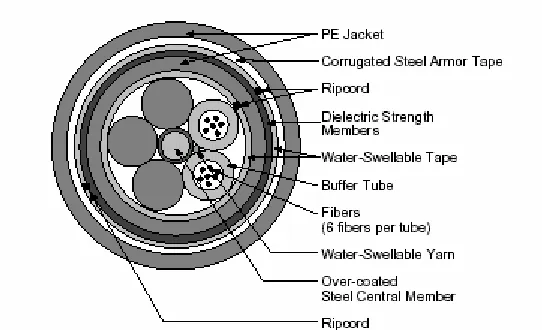
The following figure represents a cross section of a finished cable. The illustration

shown is of an armored cable with a total of twelve fibers. The fibers are grouped

into two tubes, six fibers each. Filler tubes have been used to occupy unused tube

spaces. This is a single layer cable.

(24)

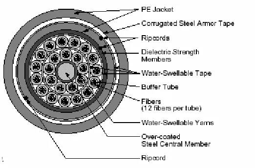
The following figure is a dual layer cable. This means that it has passed through

the Stranding department two times before being sent on to the Jacketing

department. The first pass is to assemble the inner layer of the core and the

second pass is to add the outer layer of tubes.

(25)

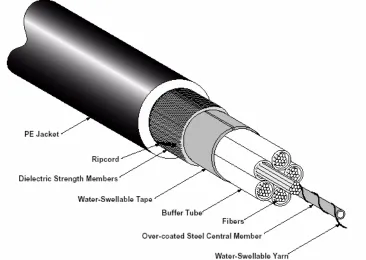
The following figure is an angled view of a single layer, five tube, and non-armored

cable.

(26)

The Problem

Any particular cable that is ordered requires a large number of setups in its

manufacture. Fiber components need one setup each in the Coloring department.

Each tube requires a setup for the tube and a setup for each fiber within that tube

in the Buffering department. Each fiber of each tube is then tested which requires a

setup for the tube and a setup for each fiber at the In-Process Testing department.

Cores need a setup for the core and a setup for each tube within each core in the

Stranding department. A setup is done for each pass through the Jacketing

department on each cable. Each setup that is performed throughout the

manufacturing process represents a loss of time and capacity.

The main purpose of this work is to determine the best way to combine orders in

the Buffering department to reduce setup requirements throughout the rest of the

manufacturing processes. Because of the nature of the required manufacturing

steps for any particular cable, combos that are made must take into account

requirements throughout the whole manufacturing process to capitalize on setup

savings. Additionally, because of raw material issues, the length of any combos

orders must be less than or equal to 13,000 meters. To accomplish this, several

(27)

First, cable orders must be divided in to groups called families. These families are

sets of orders that are identical in makeup, except for length and print. This must

be done because of the continuous nature of the extrusion process in Jacketing.

That is, once a run is started, the setup configuration cannot be changed until the

order(s) is (are) finished.

Second, within each family, smaller groups of orders, called subfamilies, must be

identified. A group of orders within a subfamily shares the same requirements from

the Jacketing perspective since they are taken from the same family. In addition, a

subfamily is composed of orders that share “equivalent” tube layouts. That is, both

tubes must be of the same diameter, the same color, and have the same number

of fibers within. Since some orders use filler tubes as a placeholder for lower tube

count orders, a filler tube may be considered equivalent to any other tube.

As an example, suppose there are two orders with five position cores. The first

order requires five tubes and the second only requires four tubes. The 5th position on the second order will be a filler tube. That filler tube is considered to be

equivalent to the 5th tube on the first order. Those cores may then be combined into one long order, provided the other four tubes are identical and that the sum of their

(28)

Third and finally, within each subfamily, combinations of orders must be explored to

determine the best possible way to meet order requirements while minimizing the

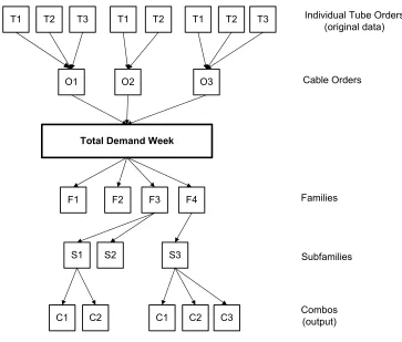
number of setups needed. An abbreviated schematic representation of the problem

has been included below.

T1 T2 T3 T1 T2 T1 T2 T3

O2 O3

O1

Total Demand Week

F1 F2 F3 F4

S1 S2 S3

C1 C2 C1 C2 C3

Individual Tube Orders (original data)

Cable Orders

Families

Subfamilies

Combos (output)

(29)

The figure above is a representation of the breakdown of processes that must be

performed on the data. Any real instance of data would entail thousands of tube

orders instead of the handful that are represented here. This is presented only as a

means to visually represent the transition between data processing stages.

At the top of the diagram are the raw, individual tube orders. Groups of these tubes

together are part of individual cable entries, which are represented with the second

row of boxes. The entire group of these cables makes up the total demand for a

manufacturing week. This group is then sorted into groups that share similar

manufacturing requirements in the Jacketing department, called families. Each

family is then further divided into subfamilies based on tube configuration, which is

important in the Stranding department. Finally within each subfamily, we will

explore combinations of orders in an effort to reduce setup requirements.

In summary, families are groups of orders with identical Jacketing department

requirements. Subfamilies are groups with identical requirements in the Stranding

department. Since we will only explore combinations for the Buffering department

within each subfamily individually, we have taken into account the manufacturing

(30)

Mathematical Modeling

To reduce setup requirements, orders should be combined wherever possible. In

other words, the number of individual combos, and therefore setups, created

should be minimized. To accomplish this as many orders as possible should be

grouped into combos. Those combos, however, must be restricted in length to a

maximum of 13,000 meters.

Let wi be the length of the ith order

N be the total number of orders that must be manufactured

W be the sum of the lengths of all N orders

Xij be 1 if order i is in combo j; 0 otherwise

J be the total number of combos created

L be the maximum length of a combo; 13,000 meters

The order of complexity for determining the best possible combo from N orders

with complete enumeration is O(2N_{) which represents the sum of all 1-order}

combinations, 2-order combinations, 3-order, etc. up to N-order combinations. This

must be done at least W / L times for each subfamily. Because the number of

(31)

One basic formulation of this problem in the context of dynamic programming is as

a value independent linear knapsack problem or stock cutting problem. A stock

cutting problem may be stated as an integer linear program as follows.

j x L x w t s x w j n j j j n j j j ∀ = ≤

∑

= = 1 , 0 . . max 1 1

where: wi is the length of the ith order, L is the maximum allowable combo length,

and Xi is 1 if the ith order is used and 0 otherwise.

The traditional dynamic programming approach to a knapsack problem is to form

ratios of weight to volume or in this case weight to length. The items are then

selected in decreasing ratio order as long as is feasible. However, in this case,

because the ratios are identical for all orders, there is no clear distinction between

(32)

To overcome this difficulty, we elect to partition the problem as a series of modified

dynamic programming problems. Before introducing the modifications necessary

for this particular setting, the traditional partition problem formulation is explained.

As an example consider a 2-partition problem to determine whether a subset of

orders exists such that the sum of the weights of the subset is equal to exactly one

half the sum of the weights of the entire set of orders. The traditional formulation is

a true-false matrix where 1 indicates true and 0 indicates false.

Given a set of n orders

let:

Wi be the weight of the ith order

B equal the total weight of all n orders

L be half the weight of B: L = B/2 = B/n

k designate the index

v(i,k) = 1 if the subset sum equals k, 0 otherwise

To build the partition matrix, weights are ranked in non-decreasing order. The

iteration is initiated with

 

 =

=

otherwise 0

w k if 1 k)

(33)

That is the first row of the matrix has a single non-zero entry in column k = w1. The

second row is created with the use of the following equation.

v(2,k) = max{ v(1,k-w2), v(1,k),v(2,w2)=1}

The second row consists of 1’s at k = w2, anyplace that 1’s exist in the row above,

in this case w1, and also w2 units positive offset from the 1’s in the previous row.

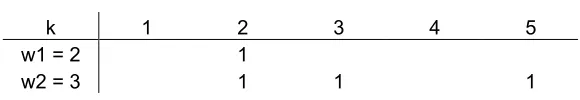
As a small example, assume w1 = 2 and w2 = 3. Then in row 1 the matrix is all 0’s

except column k = 2. In row 2, all entries will be zero except k = w2 = 3, or

wherever there is a 1 in the row above, in this case 2, and also offset from that

column 3 units, the weight of w2, to 5. These results are shown in tabular form.

Table 2: Example Matrix Partition

k 1 2 3 4 5 w1 = 2 1

w2 = 3 1 1 1

(34)

v(i,k) = max{ v(i-1,k-wi), v(i-1,k), v(i,wi)=1}

The procedure will terminate in one of two ways. If v(i,L) = 1 for any i then there

exists a partition. If v(i,L) = 0 ∀ i then no subset exists in which the sum of the

weights equals one half the sum of the entire set’s weights, i.e. no partition exists.

For the problem in this particular setting we are not interested in merely the

existence of a subset comprising half the total weight of the orders. Rather, we are

interested in finding subsets in which the sum of its weights is as close as possible

to L. As an integer linear program, the problem may be stated as follows:

j i x x L x w t s J ij J j ij n j ij i , 1 , 0 1 . . min 1 1 ∀ = = ≤

∑

= =

We wish to minimize the number of combos that are created, indicated by J. Any

(35)

meters. Any particular order must be assigned to a combo and may only be

assigned to a single combo. With this objective in mind, we can now introduce the

modifications to the traditional partition problem that are needed for our problem.

First we begin by forming subsets in the same manner as a partition problem

except we accumulate lengths in decreasing order instead of non-decreasing order

as in the unmodified partition problem.

This modification was discovered during the development phase of the combo

optimizer. We noticed that the first few combos formed were very good, that is

optimal or close to optimal. However, as the procedure continued, the remaining

combos were composed of single orders that were typically greater than 7,000

meters. Unfortunately there were no orders remaining that were short enough to

combine with these longer cables. We had “used up” all of the short orders. By

sorting the orders in decreasing lengths we were able to address this problem in a

test environment.

The DP terminates when either we have run through all the possible combinations

or when we find a subset that exactly equals L. In either case, the best combination

is annotated and the orders are removed from further consideration. In this context,

the best combination is the set that makes up the combo that is of a length as close

(36)

Once the orders making up a combo have been removed from the set under

consideration, a new DP is initiated. This cycle continues until all orders have been

assigned to combos. Each combo created with the DP corresponds to a particular

instance of j in the length constraint of the integer linear program above.

Finally there is one more level of complication that must be added to the problem to

fully represent the true system. Not only do we wish to minimize the number of

combos that must be made in order to minimize setups, we also must take into

account the number of tubes each of the individual orders represents. Therefore,

we rank cables in decreasing number of tube orders and then by decreasing

lengths within each group of orders with the same number of tubes. In this way we

stand to gain the greatest benefit of associating higher tube count orders with each

other before adding the consideration of lower tube count orders.

As an example, by combining 2 five-tube orders, 5 tube setups and one cable

setup are saved. Combining a five-tube order with a three-tube order saves 3 tube

setups and one cable setup. Therefore it is advantageous to maximize the

combination of orders with the higher number of tubes whenever possible.

That is not to say, however, that no combos will be made with different numbers of

(37)

only then will we consider the maximization of including lower tube count orders as

well.

The order of complexity for a partition based dynamic program is determined by the

number of elements in the set of orders and the size of the partition. In this

modified case, the number of orders is N, and the size of the partition desired is the

maximum length of a feasible combo, 13,000 meters. The DP must be repeated

until all orders have been assigned to combos. This is done a minimum of W/L

times, which is the total length of the orders in the subfamily divided by the

maximum combo length. W/L also forms a lower bound on the optimal number of

combos that can be determined by the modified DP. Therefore, the order of

complexity for each subfamily is O(NLW/L) = O(NW).

This order of complexity is a worst-case based assessment. To reach such

extremes, it must be true that at no time during the exploration of subsets, was

there ever a combination that met the optimality conditions. One example would be

if no two orders summed to less than 13,000 meters in length. Although this does

occur in subfamilies with small numbers of members, in larger groups of orders, the

probability of this occurring has been empirically observed to be negligible.

In summary, the approach we use to determine optimal combinations of orders is

(38)

determined by a single DP instance that corresponds to one length constraint in the

ILP. A series of dynamic programs will be used for each subfamily until all orders

are assigned to combos. Finally, each subfamily requires a series of dynamic

programs.

The amount of computation required precludes any use of a hand calculation

based approach. The determination of families alone is based on comparisons of

over a dozen attributes of cable orders with several million possible permutations.

Even constructing a single partition DP instance can quickly become cumbersome

if one is considering more than a few orders simultaneously. An automated solution

will be used.

Solution

We have developed a computer program that performs all the tasks necessary to

determine which orders should be combined to reduce setup requirements. This

program is composed of two parts. One is written in VB and acts as the front end,

data preparation tool, and output creator. The other is written in FORTRAN and

(39)

VB Program Outline

I. Read Data file

a. Initiate arrays with first tube order

b. Read next tube order

c. Determine if this is part of a cable order already processed

i. Yes: Append tube info

ii. No: Start a new cable entry

II. Determine Families

a. Initiate family count with first order

b. Check equivalency on rest of orders; mark as same family if

equivalent

c. Move to next unassigned cable and repeat

III. Determine subfamilies

a. Assign first cable as first subfamily

b. Check equivalency on rest of orders

i. Equivalent family

ii. Equivalent tube composition

1. Two live tubes identical

2. Single live paired with filler

c. Move to next unassigned cable and repeat

(40)

a. Sort by family: increasing

b. Sort by subfamily: increasing

c. Sort by number of tubes: decreasing

d. Sort by length: decreasing

V. Parse each subfamily to the Fortran Optimizer

a. Create Optimizer source file with first subfamily

b. Hold till Optimizer finishes

c. Read Optimizer results

d. Move to next undone subfamily and repeat

VI. Output Results

a. Sort Arrays by Combo

b. Create Final Output text file

Fortran Program Outline

I. Read temp data file (one subfamily, sorted)

a. Retain order info in arrays

i. Index

ii. Length

iii. Number of tubes

(41)

II. Build the partition DP

a. Start with highest number of tube orders

b. Accumulate lengths by building matrix rows for all orders of current

tube count

c. Determine if more orders are needed in the partition matrix

i. No: move on to backtrack

ii. Yes: move to next lower tube count and repeat

III. Backtrack

a. Determine the path of the best solution

i. Locate the best combo in lower right of matrix

b. Annotate the proper orders

i. Cycle back through partition using length of orders

1. Determine if order was used in combo

a. Yes: mark for removal

b. No: move to next order

IV. Move through marked orders

a. Attach current combo number to order

b. Write index number and combo number to temp output file

c. Collapse matrix by removing combo orders

V. Rebuild the partition matrix

a. Determine whether more orders need to be included in the matrix

(42)

ii. No: repeat backtrack

b. Continue cycle until all orders assigned

T1 T2 T3 T1 T2 T1 T2 T3

O2 O3 O1

Total Demand Week

F1 F2 F3 F4

S1 S2 S3

C1 C2 C1 C2 C3

(VB) Read Data

and Populate Arrays

(VB) Determine Families

by

Jacketing Requirements

(VB)

Determine Subfamilies by

Stranding Requirements

(VB to FORTRAN) Shell To Optimizer

FORTRAN 1

FORTRAN 2

(43)

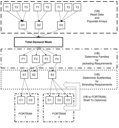
We revisit the previous illustration in the modified figure above for clarification of

the optimizer objectives. The figure above illustrates the breakdown of data

progression throughout the stages of optimization and the areas of the procedure

that are controlled by each portion of the optimizer program. Each group of combos

created from a single subfamily represents a single invocation of the FORTRAN

coded DP. The subfamily information is passed to the optimizer and the results are

passed back to the VB shell upon completion of combo determination. This cycle

repeats until all subfamilies have been processed upon which time the VB program

will continues onto final output presentation.

Approximation

The FORTRAN optimizer does the required computations on information which

represents the original data in terms of the nearest 10-meter increment. An order of

8234.62 meters is rounded up to 8240 meters. This is then retained as 824

10-meters.

This rounding enables the reduction of memory and computational requirements

within the FORTAN optimizer by a factor of ten. This greatly speeds the

(44)

opportunity for a better optimization by rounding the data. However empirical

evidence indicates that this is not an issue of any realistic concern. The data used

during the development of the program was tested with both 10-meter and 1-meter

increments. The runtime increased but there was no observable difference in the

results between the two experiments on nearly 200 subfamilies.

Results

We have used two different types of scenarios to test the effectiveness of the tube

combo optimizer program. One is typical of a high volume demand level that

utilizes nearly all the available manufacturing capacity. The other is typical of a

lower demand level that is more representative of the current business situation.

The nature of the optimizer is such that as the number of orders is increased, the

potential for savings is also increased. This is due to the simple fact that with more

orders there will come more possible combinations of orders and therefore more

(45)

High Volume Scenario

First we look at a high demand level order week. Proprietary concerns prohibit the

presentation of actual order information. Instead a summary of results is presented

in the following table.

Table 3: High Volume Order Comparison

Individual Tube Orders (Original) 3947 Individual Tube Orders (Optimizer) 2189

Cable Orders (Original) 830 Cable Orders (Optimizer) 418

Tube Setups Saved vs. Original 1758

Cable Setups Saved 412

The optimizer was able to reduce the number of necessary tube setups by 45%.

(46)

Taking the total length within each subfamily and dividing it by the value of the

maximum combo length of 13,000 meters easily determines the absolute lowest

number of combos that could have been created. For example, one particular

subfamily totals 92939.62 meters in length. 92939.62 divided by 13,000 equals

7.14 which is then rounded up to 8. Therefore the theoretical best that can be done

with that subfamily is to combine all the orders into 8 combos. As it happens, the

optimizer did identify 8 combos.

Overall, the theoretical best for the entire high volume data set is 397 combos. The

optimizer created 418 combos, which represents only a 6% deviation from the

theoretical best result. It should be noted that the absolute worst-case scenario that

could happen with any subfamily is that there exists no combo possibilities. In that

case the number of setups would exactly equal the number of tube orders.

Lower Volume Scenario

A more recent data set was used as a basis for a direct comparison to actual

manufacturing efforts. This set is representative of a typical manufacturing week

under reduced demand loads as have been experienced recently. Even with the

reduction of demand levels, the optimizer was able to find considerable untapped

(47)

Table 4: Recent Demand Level Comparison

Individual Tube Orders (Original) 1454 Individual Tube Orders (Actual) 1180 Individual Tube Orders (Optimizer) 927

Cable Orders (Original) 297 Cable Orders (Actual) N/A Cable Orders (Optimizer) 179

Tube Setups Saved vs. Original 527 Tube Setups Saved vs. Actual 253 % Length increase vs. Original 46% % Length increase vs. Actual 25%

The term original in the table above is to denote quantities before any combo

determinations are made, i.e. raw data numbers. Actual is a term used to denote

what was actually run on the manufacturing floor by using their existing scheduling

tools and finally, optimizer is a term for what would have been possible if the tube

optimizer were used to determine combos. The optimizer was able to find a 22%

reduction in the number of necessary tube setup compared to what was

(48)

Impact

Reuben Cannon, our primary contact at Corning Cable Systems, Winston-Salem

has offered some comments concerning what the tube combo optimizer would be

able to contribute to their manufacturing efforts.

“The project, optimization of the order combos, was initiated to realize equipment capacity being consumed in set up times in order that overall plant capacity could be increased at a lower rate than the industry growth rate. In short this means that we found ourselves resource constrained and needed extra capacity from our existing equipment. We have also found that the benefits of the project when operating at less than rated capacity is a much better utilization of the operators with much more flexibility allowed in the production process. Based on the different benefits stemming from the same source, setup time reduction, I break down the benefits according to the business load.

High Load

In a heavily loaded business condition, the production machines become very heavily loaded and pushed to their rated capacity. Since the rated capacity

includes both set up and run time, we must reduce one or both of these in order to process more orders and reap the benefits. The run time is often a design feature of the process equipment and hence has very little variability or upside. This leaves us with the amount of time and resources lost to set up. The surest method of reducing a set up is by eliminating one and hence the benefits of the combo optimizer. By standardizing the combination process while at the same time reducing the time it takes for the solution to be generated, we allow the factory to schedule in smaller increments and consider more solution sets resulting in better flexibility to handle expedited orders and unplanned orders such as scrap and rework. The scheduler is now able to consider more solutions and find better combinations instead of finding one which falls into an acceptable group according to the rules.

Light Load

In a lightly loaded plant, the best utilization of operators is the key to success. The optimizer allows us to maximize the run lengths, minimize the set up times while at the same time searching through more solution sets to find a better match a single scheduling solution generation process will allow. Although the number of

(49)

The data comparisons reveal a 25% increase in combined order lengths. The comparisons were done between actual solutions generated in single processes and those created by the optimizer. This percentage of setup time is now directly applicable to other areas of focus in the plant or our ability to reduce variable labor cost.

Overall, the project has demonstrated great potential savings opportunities by further enhancing successful plant procedures. Rather than being limited to a single solution set, the optimizer makes many solutions available and provides that which provides us with the most beneficial run length for processing. The goal length also allows the plant to process closer to raw material lengths and hence reduces the material leftovers which impact scrap and setup time associated with reuse of such materials. Bottom line, the optimizer allows more schedules to be generated and analyzed with less resources for a cost savings in the resulting scheduling solutions.”

Future Work

The development of this program was a modular and iterative process. While

analyzing the results of early efforts in the FORTRAN module, we recognized the

deficiency of ranking orders in non-decreasing length arrangement. Although the

concept of better performance has been explored in a test environment, it has not

been fully implemented into the tube optimizer program. This would entail a

modular change of the FORTRAN portion of the package.

There will be some required changes in order to implement the optimizer with

legacy systems at Corning Cable Systems. Such efforts would include the addition

(50)

through appropriate database and/or file selection. This could allow a rolling

schedule based approach to manufacturing efforts.

The impact of the optimizer will not only affect downstream processes as

mentioned, but will also affect the required lengths for fiber supply. Ideally a system

such as this should incorporate current fiber inventory position into its decision

process to fully optimize the entire system performance. Some coordination of

information between the tube optimizer and fiber inventory status should be

(51)

References

Bellman, Richard E. and Dreyfus, Stuart E. (1962), Applied Dynamic Programming, Princeton University Press

Hodgson Thom J., Jackson, Steven D., Qu Peijun, Cannon, Reuben E. (2001), A Material Allocation Scheme for Optical Fiber Cable Manufacturing, submitted to International Journal of Production Research, Integrated Manufacturing Systems Engineering Institute, North Carolina State University

Kosur, Anand (2001) The Tube Combos Project, Unpublished ME in Integrated Manufacturing Systems Engineering, North Carolina State University, Raleigh

Nemhauser, George L. (1966), Introduction to Dynamic Programming, New York: John Wiley and Sons Inc.

http://www.corningcablesystems.com/web/library/litindex.nsf/Cable?OpenView&Sta

(52)

(53)

FORTRAN Code

************************************************************************ ** Corning Combo Scheduling System ** ** Programmed by: Thom Hodgson ** ** Stu Miller ** ************************************************************************ ** length (i) length of order i ** ** klen (i) length of order i used in dynamic program ** ** notubes(i) number of tubes in order i ** ** orderid(i) identification # of order i ** ** f (m,k) dynamic program function ** ** id(m,k) dynamic program index ** ** first(nt) pointer to first order with 'nt' tubes ** ** last (nt) pointer to last order with 'nt' tubes ** ** uniqueid(i) external identifier of order i ** ************************************************************************ integer length(1000),notubes(1000),first(24),last(24),

. klen(300),nindex(300),f(300,1301),uniqueid(1000), . id(300,1301),totlen

logical switch,used(1000)

open(1,file="Fcombosource.txt",status="old") open(2,file="Fcomboout.txt",status="unknown") maxlength = 1300

******read data********************************************************* do i = 1,10000

read(1,*,err=99,end=1) uniqueid(i),flength,notubes(i) length(i) = flength/10.+1.0

end do

1 n = i-1 ! n holds number of orders read

******set up pointers by #tubes***************************************** do i = 1,24

first(i) = 0 end do

do i = 1,n ! cycle thru orders, set up pointers (first, last) nt = notubes(i)

if(first(nt).eq.0) then !is this 1st order with 'nt' tubes? first(nt) = i ! hold order number in first and last last (nt) = i

(54)

end if end do

******do first heuristic, starting with largest #tubes****************** j = 0

ncombo = 0 totlen = 0

do nt = 24,1,-1 ! */*/*/*/*/*/* Big Loop if(first(nt).eq.0) cycle ! skip loop if no orders i1 = first(nt)

i2 = last (nt)

******get data for D.P.******

if(totlen.lt.maxlength) then ! room in the knapsack? do i = i1,i2 ! go thru all

j = j+1 ! hold number of orders under consideration klen(j) = length(i) ! hold length of individual totlen = totlen+klen(j) ! accumulate length nindex(j) = i ! pointer index end do

end if

if(totlen.lt.maxlength) cycle ! cycle out of Big Loop ******start D.P. ******

maxlength1 = maxlength+1 ! index shift to avoid zero row do while(totlen.ge.maxlength) ! */*/*/*/*/*/* Middle Loop ncombo = ncombo+1 ! hold current combo number minlen = 999999

do i = 1,j

if(klen(i).lt.minlen) minlen = klen(i) ! find min do k = 1,maxlength1

f (i,k) = 0 ! clear matrices id(i,k) = 0

end do end do

minlen1 = minlen+1 ! holds minimum of considered orders do k = klen(1)+1,maxlength1 ! initialize with first order f (1,k) = klen(1)

id(1,k) = 1 end do

if(j.gt.1) then ! more than one order under consideration? do m = 2,j

do k = 1,klen(m)

f(m,k) = f(m-1,k) ! copy prev. order values till length end do

do k = klen(m)+1,maxlength1

(55)

if(f(m,k).gt.f(m-1,k)) id(m,k) = 1 ! indicates usage end do

end do end if

******backtrack D.P.****** do i = 1,j

used(i) = .false. ! initialize with all as non-used end do

do k = maxlength1,1,-1

if(f(j,k).gt.0) exit ! find lower right with non zero value end do

totlen = 0 do m = j,1,-1

if(id(m,k).eq.1) then ! this order used in current optimal? k = k-klen(m) ! back through DP used(m) = .true. ! indicate that order on optimal path totlen = totlen+klen(m) ! accumulate length of combo end if

end do

******output combo****** do i = 1,j

if(.not.used(i)) cycle

write(2,*) uniqueid(nindex(i)), ncombo end do

******resetup active list****** k = 0

totlen = 0 do i = 1,j

do while(used(i+k))

k = k+1 ! counts used orders end do

if(i+k.gt.j) exit

totlen = totlen+klen(i) klen (i) = klen (i+k)

nindex(i) = nindex(i+k) ! collapse the pointers used (i) = used (i+k)

used(i+k) = .false. if(i+k.eq.j) exit end do

if(i+k.eq.j) then ! deal with last j = i

(56)

end do !*** End Middle Loop end do !****** End Big Loop ******final combo output******

if(j .ge. 1) then totlen = 0 do i = 1,j

totlen = totlen+klen(i)

write(2,*) uniqueid(nindex(i)), ncombo+1 end do

end if *************** stop

(57)

VB Code

Option Base 1 Option Compare Text

Private Sub Form_Load() ' */*/*/ start program

' *** variable definitions

' data fields

Dim ORDERNBR(1500) As String 'unique identifier Dim FONBR As String

Dim FOLINE As Single

Dim MARKUOM(1500) As String 'feet or meters Dim SHIPDATE(1500) As String 'due date ? Dim TUBESIZE As Integer

Dim COREOD(1500) As Single ' outer diameter of the core Dim JACKDESC(1500) As String 'armor, lite, duct etc

Dim FIRSTPASS(1500) As Single 'OD of cable after first pass Dim SECONDPASS As Single

Dim THIRDPASS As Single

Dim CMTYPE(1500) As String 'steel or grp

Dim CMSIZE(1500) As Single 'diameter of central member Dim STRIPECLR(1500) As String 'color of stripe on jacket Dim NBRSTRIPES(1500) As Integer '# of stripes on jacket Dim SBMARKREQD(1500) As String 'switchback/ROL cable flag Dim MFGDATE(1500) As String 'date cable enters manufacturing? Dim MAXFIBERS As Integer

Dim COLFIBTYP As String

Dim ORDERLENGH(1500) As Single 'length of cable required Dim FIBERCOUNT As Integer

Dim KANBANCELL(1500) As Integer 'kanban cell number cable is assigned to Dim KANBANSEQ As Integer

Dim FGPartNbr As String

Dim KS2FIBTYP(1500) As String 'identifies primary type of fiber used Dim SecondFiberType(1500) As String 'identifies secondary fiber type used Dim ITMID(1500, 24) As String 'code for color, material, size, fiber count of tube Dim ITMDESC As String

' add ons

Dim index(1500) As Integer 'array pointer index

Dim family(1500) As Integer 'keeps track of cable family number Dim subfamily(1500) As Integer 'keeps track of sub-family number Dim numberoftubes(1500) As Integer ' number of tubes required for order Dim combonumber(1500) As Integer

'temp holders

(58)

Dim tempFOLINE As Single Dim tempMARKUOM As String Dim tempSHIPDATE As String Dim tempTUBESIZE As Integer Dim tempCOREOD As Single Dim tempJACKDESC As String Dim tempFIRSTPASS As Single Dim tempSECONDPASS As Single Dim tempTHIRDPASS As Single Dim tempCMTYPE As String Dim tempCMSIZE As Single Dim tempSTRIPECLR As String Dim tempNBRSTRIPES As Integer Dim tempSBMARKREQD As String Dim tempMFGDATE As String Dim tempMAXFIBERS As Integer Dim tempCOLFIBTYP As String Dim tempORDERLENGH As Single Dim tempFIBERCOUNT As Integer Dim tempKANBANCELL As Integer Dim tempKANBANSEQ As Integer Dim tempFGPartNbr As String Dim tempKS2FIBTYP As String Dim temp2ndFiberType As String Dim tempITMID As String

Dim tempITMDESC As String

' flags and counters Dim flag As Integer Dim swap As Integer

Dim sameorderflag As Integer

Dim cables As Integer 'keeps track of number of cables in array Dim i As Integer

Dim j As Integer Dim k As Integer

Dim subfamilycounter As Integer 'keeps track of number of different subfamilies in array Dim familycounter As Integer 'keeps track of number of different families in array Dim sametubes As Integer 'keeps track of identical tubes between orders Dim numbersubfamily(1000) As Integer

Dim lengthsubfamily(1000) As Single Dim useflag(1000) As Integer

Dim combo As Integer Dim ordernumber As Integer Dim comboset As Integer ' *** end variable definitions

(59)

combonumber(i) = 0 Next i

'*** end initialize

'*** read data

cables = 1 'assuming here that file exists and has at least one entry

Open "C:\Documents and Settings\Owner\My Documents\allinone\VBsourcedata.txt" For Input As #10 'open and read first data line into arrays

Input #10, ORDERNBR(1), FONBR, FOLINE, MARKUOM(1), SHIPDATE(1), TUBESIZE, _

COREOD(1), JACKDESC(1), FIRSTPASS(1), SECONDPASS, THIRDPASS, CMTYPE(1), _ CMSIZE(1), STRIPECLR(1), NBRSTRIPES(1), SBMARKREQD(1), MFGDATE(1), MAXFIBERS, _

COLFIBTYP, ORDERLENGH(1), FIBERCOUNT, KANBANCELL(1), KANBANSEQ, FGPartNbr, _ KS2FIBTYP(1), SecondFiberType(1), ITMID(1, 1), ITMDESC

index(1) = 1 'setting first element indicates there is at least one cable

numberoftubes(1) = 1 'setting first element indicates that there is one tube so far

Do Until (EOF(10) = True)

sameorderflag = 0 'flag for order equivalency

Input #10, tempORDERNBR, tempFONBR, tempFOLINE, tempMARKUOM, tempSHIPDATE, _ tempTUBESIZE, tempCOREOD, tempJACKDESC, tempFIRSTPASS, tempSECONDPASS, _ tempTHIRDPASS, tempCMTYPE, tempCMSIZE, tempSTRIPECLR, tempNBRSTRIPES, _ tempSBMARKREQD, tempMFGDATE, tempMAXFIBERS, tempCOLFIBTYP,

tempORDERLENGH, _

tempFIBERCOUNT, tempKANBANCELL, tempKANBANSEQ, tempFGPartNbr, _ tempKS2FIBTYP, temp2ndFiberType, tempITMID, tempITMDESC

' read into temp holders

For i = 1 To cables 'loop through all previous entries

If (tempORDERNBR = ORDERNBR(i)) Then 'is new(temp) same as current(i)? numberoftubes(i) = numberoftubes(i) + 1 'increment # of tubes for order

ITMID(i, numberoftubes(i)) = tempITMID 'append the item ID on the end of the order sameorderflag = 1 'trip flag to escape long assignment block coming up

i = cables 'get out of this loop End If

Next i

If (sameorderflag = 0) Then 'means this is a new cable entry cables = cables + 1 ' increment the number of cables 'copy the temp holders into the array in the next position ORDERNBR(cables) = tempORDERNBR

FONBR = tempFONBR FOLINE = tempFOLINE

MARKUOM(cables) = tempMARKUOM SHIPDATE(cables) = tempSHIPDATE TUBESIZE = tempTUBESIZE

(60)

SECONDPASS = tempSECONDPASS THIRDPASS = tempTHIRDPASS CMTYPE(cables) = tempCMTYPE CMSIZE(cables) = tempCMSIZE

STRIPECLR(cables) = tempSTRIPECLR NBRSTRIPES(cables) = tempNBRSTRIPES SBMARKREQD(cables) = tempSBMARKREQD MFGDATE(cables) = tempMFGDATE

MAXFIBERS = tempMAXFIBERS COLFIBTYP = tempCOLFIBTYP

ORDERLENGH(cables) = tempORDERLENGH FIBERCOUNT = tempFIBERCOUNT

KANBANCELL(cables) = tempKANBANCELL KANBANSEQ = tempKANBANSEQ

FGPartNbr = tempFGPartNbr

KS2FIBTYP(cables) = tempKS2FIBTYP SecondFiberType(cables) = temp2ndFiberType

ITMID(cables, 1) = tempITMID 'new cable has only one ITMID so far ITMDESC = tempITMDESC

numberoftubes(cables) = 1 ' one tube so far

index(cables) = cables 'set the index to the current array position End If

Loop Close #10

' *** end read data

' *** itmid sorter: sorts itmid numbers for each cable: ascending For i = 1 To cables ' loop through all the orders

flag = 0

If (numberoftubes(i) > 1) Then 'if there's only one tube, no sort needed Do Until (flag = 1) ' finished?

flag = 1 ' assume finished For j = 1 To numberoftubes(i) - 1

If (ITMID(i, j + 1) < ITMID(i, j)) Then 'out of order? tempITMID = ITMID(i, j + 1)

ITMID(i, j + 1) = ITMID(i, j) ' swap positions ITMID(i, j) = tempITMID

flag = 0 ' not finished End If

Next j Loop End If Next i

' *** end itmid sorter

'

'from this point forward, elements are referenced and sorted with an indexed scheme '

(61)

flag = 1 ' assume finished For j = 1 To cables - 1

If (numberoftubes(index(j)) < numberoftubes(index(j + 1))) Then 'out of order? tempindex = index(j)

index(j) = index(j + 1) 'swap index positions index(j + 1) = tempindex

flag = 0 'not finished End If

Next j Loop

' *** end number of tubes sorter

' *** cable equivalency checker: checks each cable vs every other for same family type familycounter = 0 'initialize family counter

For i = 1 To cables - 1

If (family(index(i)) = 0) Then 'has this cable been done already? familycounter = familycounter + 1 ' increment family counter family(index(i)) = familycounter

'set current family to current count of distinct families

For j = i + 1 To cables 'loop though all other cables after current(i) If ( _

(family(index(j)) = 0) And _

(MARKUOM(index(i)) = MARKUOM(index(j))) And _ (COREOD(index(i)) = COREOD(index(j))) And _ (JACKDESC(index(i)) = JACKDESC(index(j))) And _ (FIRSTPASS(index(i)) = FIRSTPASS(index(j))) And _ (CMTYPE(index(i)) = CMTYPE(index(j))) And _ (CMSIZE(index(i)) = CMSIZE(index(j))) And _

(STRIPECLR(index(i)) = STRIPECLR(index(j))) And _ (NBRSTRIPES(index(i)) = NBRSTRIPES(index(j))) And _ (SBMARKREQD(index(i)) = SBMARKREQD(index(j))) And _ (KANBANCELL(index(i)) = KANBANCELL(index(j))) And _ (KS2FIBTYP(index(i)) = KS2FIBTYP(index(j))) And _

(SecondFiberType(index(i)) = SecondFiberType(index(j)))) Then 'same cable family? family(index(j)) = familycounter 'set equivalent cables to same family number End If

Next j End If Next i

If (family(index(cables)) = 0) Then 'check if the last order was done familycounter = familycounter + 1

family(index(cables)) = familycounter End If

' *** end cable equivalency checker

' *** tube equivalency checker: checks all cables vs every other for same tubes subfamily(index(1)) = 1 'initialize the first cable

subfamilycounter = 1 ' initialize the subfamily counter For i = 1 To cables - 1 ' outer loop

(62)

subfamily(index(i)) = subfamilycounter 'if it wasn't done it means it is a new subfamily End If

For j = 2 To cables ' inner loop

If (subfamily(index(j)) = 0 And family(index(j)) = family(index(i))) Then ' undone and same family as outer loop ?

sametubes = 0 'reset counter of same itmid() numbers

For k = 1 To numberoftubes(index(i)) ' loop thru itmid();assume #(i) >= #(j) If (ITMID(index(i), k) = ITMID(index(j), k)) Then 'identical tubes? sametubes = sametubes + 1 ' increment counter

Else

If (ITMID(index(j), k) <> "" And (ITMID(index(i), k) <> ITMID(index(j), k))) Then ' not a filler tube and not an identical tube

sametubes = 0

k = 99 ' arbitrary large number to jump out of loop End If

End If Next k

If (sametubes > 0) Then ' means combo possibility subfamily(index(j)) = subfamily(index(i))

End If End If Next j Next i

If (subfamily(index(cables)) = 0) Then 'check if the last order was done subfamilycounter = subfamilycounter + 1

subfamily(index(cables)) = subfamilycounter End If

' *** end tube equivalency checker

'*** 4 level sorter: family,subfamily,numberoftubes,orderlengh: ascending flag = 0 'initialize flag

Do Until (flag = 1) ' finished? flag = 1 ' assume finished For j = 1 To cables - 1 swap = 0 'assume in order

If (family(index(j)) < family(index(j + 1))) Then swap = 1 'out of order

Else

If (family(index(j)) = family(index(j + 1))) And _ (subfamily(index(j)) < subfamily(index(j + 1))) Then swap = 1 'out of order

Else

If (family(index(j)) = family(index(j + 1))) And _ (subfamily(index(j)) = subfamily(index(j + 1))) And _

(numberoftubes(index(j)) < numberoftubes(index(j + 1))) Then swap = 1 'out of order

Else

If (family(index(j)) = family(index(j + 1))) And _ (subfamily(index(j)) = subfamily(index(j + 1))) And _

(63)

End If End If End If End If

If (swap = 1) Then flag = 0 'not finished

tempindex = index(j) 'switch positions index(j) = index(j + 1)

index(j + 1) = tempindex End If

Next j Loop

' *** 4 level sorter

' *** output index accumulator: cycle orders, count & accumulate length by subfamily For j = 1 To subfamilycounter ' initialize counters and indexes

numbersubfamily(j) = 0 lengthsubfamily(j) = 0 Next j

For j = 1 To cables

numbersubfamily(subfamily(j)) = numbersubfamily(subfamily(j)) + 1 'count cables by subfamily

lengthsubfamily(subfamily(j)) = lengthsubfamily(subfamily(j)) + _ ORDERLENGH(j) 'accumulate length by subfamily

Next j

' *** output index accumulator

' *** ouput to Fortran optimizer loop comboset = 0

For i = 1 To subfamilycounter

Open "C:\Documents and Settings\Owner\My Documents\allinone\Fcombosource.txt" For Output As #20

For j = 1 To cables

If (subfamily(index(j)) = i) Then 'cable part of current subfamily?

Write #20, j, ORDERLENGH(index(j)), numberoftubes(index(j)) 'send to optimizer End If

Next j Close #20

comboset = comboset + 100

' *** Shell to optimizer: calls the fortran DP and halts VB process until it returns ChDir App.Path

frmRun.Visible = False frmRun.Show

frmRun.Hide Unload frmRun

' *** end Shell to optimizer

Open "C:\Documents and Settings\Owner\My Documents\allinone\Fcomboout.txt" For Input As #30 Input #30, ordernumber, combo 'read 1st optimizer result

Dynamic Programming Based Approach to Scheduling in the Fiber Optic Cable Industry

Abstract

Biography

Acknowledgements

Table of Contents

Index of Tables

Index of Figures

Introduction

Previous Work

Manufacturing Phases

Overview

Fiber Receiving and Storage: Fiber Chamber

Coloring

Buffering

In-Process Testing

Extra Fiber Length Testing: EFL Testing

Stranding

Jacketing

Final Test

Cable Illustrations

The Problem

Mathematical Modeling

∑

∑

∑

∑

Solution

VB Program Outline

Fortran Program Outline

Approximation

Results

High Volume Scenario

Lower Volume Scenario

Impact

Future Work

References

FORTRAN Code

VB Code