by
Neil Kitney
Thesis submitted for the degree of Doctor of Philosophy in The Faculty of Engineering, University of London
Department of Mechanical Engineering
University College London
All rights reserved
INFORMATION TO ALL USERS
The quality of this reproduction is dependent upon the quality of the copy submitted.
In the unlikely event that the author did not send a complete manuscript and there are missing pages, these will be noted. Also, if material had to be removed,
a note will indicate the deletion.
uest.
ProQuest 10006777
Published by ProQuest LLC(2016). Copyright of the Dissertation is held by the Author.
All rights reserved.
This work is protected against unauthorized copying under Title 17, United States Code. Microform Edition © ProQuest LLC.
ProQuest LLC
789 East Eisenhower Parkway P.O. Box 1346
Catenary moored ship and offshore structures exhibit large amplitude horizontal oscillations caused by low frequency components of the environmental loading, due to waves, wind and current, at the system resonant frequency.
As a result of these large oscillations the mooring lines can undergo significant motion inducing large hydrodynamic drag forces. In many situations this line loading provides the major damping mechanism and reduces the resonant response of the floating vessel. The ability to predict induced mooring line tensions with accuracy, and the contribution of mooring line damping to total system response, is therefore of relevance to the offshore industry.
Although a number of numerical models exist for the prediction of line tension and damping, the excitation of the mooring line at the point of suspension creates a complicated non-linear line response that is presently not well understood and inherently difficult to model. Given the nature of the line response, validation of numerical results with experimental data is of importance. This validation has however not been possible to date due to the extremely limited quantity of experimental data available.
This thesis presents an experimental investigation into the response of small and large scale, single chain catenary mooring line models subject to a comprehensive range of top end excitation parameters. Measurements from the experimental investigation are compared with results from established numerical methods and those from a time domain numerical model developed in the thesis.
I wish to acknowledge and express my gratitude to Dr D T Brown for his invaluable advice and guidance throughout this work. I would also like to acknowledge and thank Dr G J Lyons, Professor J A Witz and the technicians of the Department of Mechanical Engineering at University College London for their assistance with this project.
I am grateful for the assistance of staff and personnel of the Canal de Experiencias Hidrodinamicas de El Pardo, MADRID, Spain in the completion of large-scale model tests. In addition, I am thankful for the financial support provided by the European Union through the Training and Mobilization of Researchers - Access to Large Scale Test Facilities Programme, without which the large model scale tests would not have been possible to undertake.
Abstract 2
Acknowledgements 3
Table of contents 4
List of figures 10
List of tables 18
Nomenclature 20
1 Introduction 24
1.1 Station-keeping and moorings 24
1.2 Environmental excitation forces 28
1.3 Damping forces 28
1.3.1 Vessel damping 28
1.3.2 Mooring system damping 29
1.4 Prediction of mooring line tension and damping 30
1.5 Scope of work 31
1.6 Thesis overview 32
2 Review of previous work 41
2.1 Mooring system design 41
2.2 Influence of water depth 43
2.3 Seabed factors 45
2.4 Mooring line failure 46
2.5 Damping loads 47
2.5.1 Vessel Damping 48
2.5.2.2 Experimental modelling 52
2.5.2.3 Numerical modelling 54
3 Introduction to mooring iine response 61
3.1 Static mooring line 61
3.2 Dynamic mooring line 63
3.2.1 Line response 65
3.2.2 Damping coefficient 66
3.3 Conclusions 68
4 Experimental equipment set-up 71
4.1 Experiment sensors 71
4.1.1 Measurement of line loads and carriage position 71
4.1.2 Sensor excitation and data transmission 72
4.1.3 Signal acquisition and recording 73
4.2 Analysis of experimental data 74
4.2.1 Spectral analysis 74
4.2.2 Data process code 76
4.2.2.1 Determination of maximum tension 76
4.2.2.2 Determination of line damping 77
4.3 Experiment oscillation system 77
4.3.1 Oscillation system control 79
4.4 Calibration 81
4.4.1 Load cell calibration 81
4.4.2 Oscillation system calibration 81
5 Experimental model development 99
5.1 Selection of an appropriate prototype model 99
5.2 Scale models 100
5.3 Static and dynamic models 101
5.3.1 Concept of the static mooring line model 101
5.3.2 The experimental static model 102
5.3.3 Concept of the dynamic mooring line model 103
5.3.3.1 Drag and added mass coefficients 104
5.3.3.2 Vortex induced vibrations (VIV) 106
5.3.4 The experimental dynamic model 107
5.4 Elastic considerations 110
5.4.1 Methods for inclusion of mooring line elasticity 112
5.4.2 Experimental model elasticity 113
5.4.2.1 Elastic model design for 1:70 scale line 113
5.4.2.2 Elastic model design for 1:17 scale line 114
5.5 Conclusions 116
6 Experimental programme development 126
6.1 Model pre-tension angles 126
6.2 Experiment oscillation parameters 127
6.3 Experimental excitation and response - precautions 128
6.3.1 Component resonance 130
6.3.2 Grounded line interference 131
7.1 Analysis results 140
7.1.1 ISSC line tension results 141
7.1.2 Experimental line tension comparison with ISSC results 142
7.1.3 ISSC line damping results 143
7.1.4 Experimental line damping comparison with ISSC results 144
7.2 Influence of elasticity on line tension measurement 148
7.3 Conclusions 150
8 Experimental results for wide range of excitation parameters 159
8.1 Non-dimensional variables 159
8.2 Response to variation of oscillation parameters 161
8.2.1 Dynamic tension variation with oscillation amplitude 161
8.2.2 Dynamic tension variation with oscillation period 163
8.2.3 Damping variation with oscillation amplitude and period 163
8.3 Amplitude at which tension peak occurs 165
8.4 Inelastic/elastic response to oscillation parameters 168
8.5 Response to out of plane excitation 168
8.5.1 Measured tension for HF excitation 169
8.5.2 Measured damping for HF excitation 170
8.6 Conclusions 172
9 Experimental results for range of initial pre-tension angles 9.1 Response to ISSC excitation parameters
9.2 Response to range of excitation parameters
9.3 Indicator diagrams
9.4 Response to out of plane excitation
192
192
197
198
9.5.1 Analysis and discussion of harmonic tension components 201
9.6 Conclusions 203
10 Development and application of a new numerical model 230
10.1 Numerical model development 230
10.1.1 Objectives 230
10.1.2 Numerical model characteristics 232
10.2 Numerical model detail 233
10.2.1 Structure 233
10.2.2 Input requirements 234
10.2.3 Operation 236
10.2.3.1 Reference position tuning 236
10.2.3.2 Time step progression 237
10.3 Comparison of numerical model, ISSC and experimental results 241
10.3.1 Damping predictions 241
10.3.2 Tension predictions 242
10.3.3 Indicator diagrams 243
10.4 Influence of pre-tension on numerical model results 243
10.5 Numerical model sensitivity 245
10.5.1 Pre-tension angle spatial discretization 246
10.5.2 Time step increment 246
10.6 Conclusions 247
11 Conclusions and recommendations 262
11.1 Mooring line model 262
11.2.2 Oscillation system
11.2.3 Elasticity and grounded line interference
11.3 Experimental results
11.3.1 Mooring line initial pre-tension angle of 52°
11.3.2 Mooring line initial pre-tension angle of 58° to 44°
11.4 Numerical model
11.5 Recommendations for future development
264
265
265
265
267
269
270
References 273
Appendix A -1 Experimental data process code 285
Appendix B -1 Experimental oscillation system configuration file 295
Appendix B - 2 Experimental oscillation system control code 296
Appendix C -1 Fourier analysis code 301
Appendix D -1 Numerical model QS look-up table
Appendix D - 2 Numerical model input
Appendix D - 3 Numerical model code
306
308
List of figures
Figure 1.1 Percentage of future field development using FPSs by water depth 35
Figure 1.2 Floating Production Storage and Offload (FPSO) vessel 35
Figure 1.3 Hull costs versus production rate for floating production systems 36
Figure 1.4 Vessel utilising dynamic positioning 36
Figure 1.5 Comparative costs of dynamic positioning and catenary mooring
systems 37
Figure 1.6 Mooring concepts 37
Figure 1.7 Inspection of the largest diameter mooring line presently in operation 38
Figure 1.8 Mooring line characteristics for water depth applications 38
Figure 1.9 Superposed high frequency excitation on low frequency drift force 39
Figure 1.10 Schematic representation of mooring line change in profile due to
environmental forcing 39
Figure 1.11 Restoring force for platform offset due to mean and varying wave force 40
Figure 2.1 Comparison of the properties of mooring line materials synthetic rope,
chain and wire 60
Figure 2.2 Quasi-static mooring line envelope for 20m amplitude oscillation of the suspension point about the equilibrium location 60
Figure 3.1 Chain hanging between two points under self weight 69
Figure 3.2 Catenary mooring line, with forces indicated at suspension and touch
down points 69
Figure 3.3 Components of tension at the suspension point of a mooring line with increasing excursion from the anchor 70
Figure 4.1 Load cell arrangement for 1:70 scale model 84
Figure 4.2 Shear beam load cell with schematic Wheatstone bridge arrangement 84
Figure 4.3 Load cell arrangement of 1:70 model 85
p. . c Example raw analogue signal with digital representations at different
g sample rates
p. . p Spectral analysis of 1:70 experimental data, harmonic high frequency 0 - 7
i-igure 4.oa oscillation
Figure 4.6b Spectral analysis of 1 ;70 experimental data, bi-harmonic oscillation 87
p. . ^ Spectral analysis of 1:17 experimental data, harmonic high frequency i-igure4./a oscillation
Figure 4.7b Spectral analysis of 1:17 experimental data, bi-harmonic oscillation 88
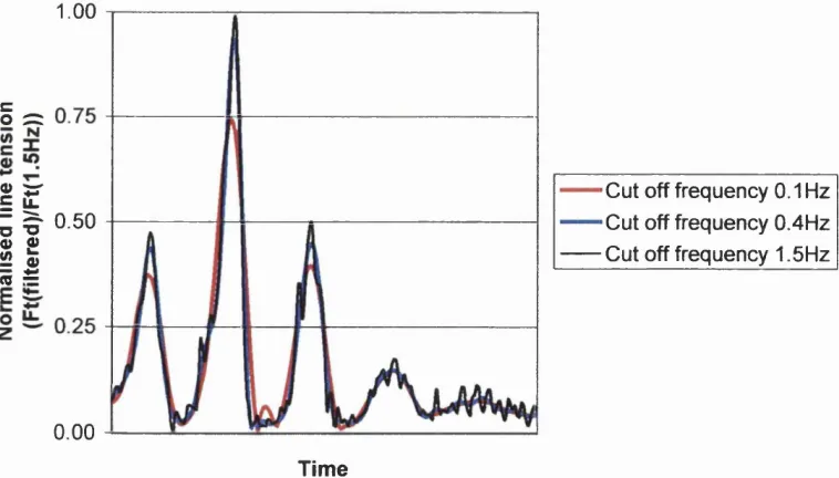
Figure 4.8 Influence of cut off frequency on line tension results 89
Figure 4.9 Influence of cut-off frequency on the tension time history 89
Figure 4.10 Example tension time history for a bi-harmonic oscillation 90
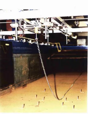
Figure 4.11 Longitudinal view along length of 1:70 model test facility 91
Figure 4.12 1:70 model test facility motion carriage 91
Figure 4.13 Perspective view of the 1:70 model test facility and chain specimen 92
Figure 4.14a Drive motor for longitudinal (planar) motion carriage of the 1:70 model 93
Figure 4 14b wheel at the end of the longitudinal carriage drive belt (1:70
Figure 4.15 Drive motor and belt for out of plane motion of 1:70 model 93
Figure 4.16 Data logging and system control area 94
Figure 4.17 Entry screen on terminal emulator for selection of oscillation type 94
Figure 4.18 General arrangement of the 1:17 model test facility 95
Piniirû/iiQ Load cell arrangement mounted from linear table assembly for 1:17
i-igure4.iy ^lodel 96
Pini iro A on Linear table assembly mounted from turret of planar motion carriage higure4.^u (i;i7m odel)
Figure 4.21 Planar motion carriage (1:17 model) 96
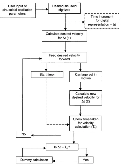
Figure 4.22 Structure of the oscillation control codes 97
Figure 4.23 Horizontal load calibration of 1:70 model load cell assembly 98
p. ,.p c 1 Drag coefficient variation with Reynolds number for smooth cylinder .p» and model scale chain specimens
Figure 5.2 Mooring line element trajectories during quasi-static oscillation 120
Figure 5.3 Static forces acting on an element of mooring line 121
p. c . Effect of seabed friction on 1:70 model mooring line quasi-static figure 0.4 tensions
Figure 5.5 Axial stiffness values from prototype scale chain data 121
Figure 5.6 Zwick tensile test machine 122
Figure 5.7 Tensile test results of 1:70 model chain specimen 122
Figure 5.8 Spring assembly for 1:70 model 122
Figure 5.9 Tensile test results of spring assembly for 1:70 model 123
Figure 5.10 Load/elongation curve for typical polyester rope, quasi-static loading 123
p. Load/eiongation curve for prototype scale synthetic mooring line, figures b .n dynamic ioading
cir..irû t;io Perspective view of the 1:17 oscillation system and spring assembly
g components
Figure 5.13 Spring assembly of 1:17 model undergoing calibration 125
Figure 5.14 Result of spring assembly calibration for 1:17 model 125
Figure 6.1 Natural period of the anchor spring assembly, quasi-static solution 137
FiniirpRp Quasi-static catenary solution for elastic and inelastic mooring line ^ tension compared with 1:70 model data
p. c o Quasi-static catenary solution for elastic and inelastic mooring line figure o.d tension compared with 1:17 model data
FiniiroRA Low frequency sinusoidal oscillation of 1:17 model with associated
^ spring response
Figure 6.5 Bi-harmonic oscillation of 1:17 model with associated spring response 139
Figure 7.1 ISSC numerical model total line tension prediction 154
FiniiroTo Experimentally measured line tension compared to ISSC numerical .g .
Figure 7.3 ISSC numerical model iine damping prediction 155
___ _ „ Experimentally derived line damping compared to ISSC numerical .
Figure 7.4 predictions ^^5
Figure 7.5 Indicator diagram for LF 10m amplitude oscillation of 100 second period 156
Figure 7.6 Indicator diagram for HF 5.4m amplitude oscillation of 10 second period 156
p. Indicator diagram for combined LF and HF oscillation at 10 and 5.4m amplitude at 100 and 10 second period respectively
Figure 7.8 Indicator diagram for HF 5.4m amplitude oscillation of 10 second period 157
p. _ Total line tension for ISSC TD and experimental elastic and inelastic .j-o Figure 7.9 rnodels
Figure 8 1 Non-dimensional dynamic tension for harmonic LF oscillations (T/Tp =
Figure 8 2 Non-dimensional dynamic tension for harmonic HF oscillations (T/Tp =
cir^.iro o Q Non-dimonsionsl dynamic tension for bi-harmonic oscillations (HF T/Tp higure ü.d ^ 0.55)
Figure 8 4 Non-dimensional dynamic tension for harmonic HF oscillations (amp/H
cTiniirûflt; Non-dimensional dynamic tension for bi-harmonic oscillations (HF higure b.b amp/H = 0.07)
cTni r oOf i Non-dimensional damping for bi-harmonic and harmonic oscillations . , 7
higure o.b (HP T/Tp = 0.55) '
Pin, ira A 7 Non-dimensional damping for bi-harmonic and harmonic oscillations
higure ü./ (HF amp/H = 0.07) ^
Piniiro ft ftc Indicator diagram for HF harmonic oscillations (amp/H = 0.07, T/Tp = ...^q
higurea.ua o.55 to 1.10) ^
Piniira ft fth lodicator diagram for HF harmonic oscillations (amp/H = 0.07 to 0.10,
higure a.ao = 0.55) '
Pin, iro ft Qo indicator diagram for bi-harmonic oscillations (HF amp/H = 0.07, T/Tp = . higure o-ya 0.55 to 1.10)
Pin, irn ft QK Indlcator diagram for bi-harmonic oscillations (HF amp/H = 0.07 to 0.10, , pn higure B.yo y/Tp = 0.55)
Pin. ft i m Location where maximum tension occurs within the excursion of a .q.
Figure 8.10 harmonic LF oscillation ^^1
FiniirA A 11 Location where maximum tension occurs within the excursion of a .p., ^ harmonic HF oscillation (varying amplitude)
pin.irno ft MO Location where maximum tension occurs within the excursion of a
bi-Figures 8.12 harmonic oscillation ^^2
Pi oMo Location where maximum tension occurs within the excursion of a .pn
P-. p . . Indicator diagram for H F Harmonic oscillations (amp/H = 0.07 to 0.10, higure a.M y/Tp = 0.55)
pvi rofl ie; Indicator diagram for HF harmonic oscillations (amp/H = 0.07, T/Tp = higure a.io o.55 to 1.10)
p. p .p Comparison of inelastic and elastic line tensions for harmonic and bi-higure o.ib harmonic oscillations (HF T/Tp = 0.55)
p. , . _ p i7 Non-dimensional dynamic tension for HF harmonic oscillations at 0°, .p .
higure a .i/ 45° and 90' (T/Tp = 0.55) °
PiniiroftiR Non-dimensional dynamic tension for bi-harmonic oscillations, HF higure a.ia component at 0°, 45° and 90° (HF T/Tp = 0.55)
Comparison non-dimensional dynamic tension from bi-harmonic line Figure 8.19 oscillations, and as constructed by summation of individual LF and HF 185
components
p. Non-dimensional dynamic tension for HF harmonic oscillations at 0°, .pp higure a.^u 4 5» and 90° (amp/H = 0.07)
Pi P«. Non-dimensional dynamic tension for bi-harmonic oscillations, HF .pp higure a.^i component at 0°, 45° and 90* (HF amp/H = 0.07).
PiniirûRoo Non-dimensional dynamic tension for HF harmonic oscillations at 0°, .p^
higure a.^^ 4 5. gnd 90° (T/Tp = 0.55) '
Pi p pq Non-dimensional damping of bi-harmonic oscillations, HF component at .p^ higure go 450 ^^d 90“ to plane of suspension (HF T/Tp = 0.55)
PiniirofiOA Non-dimonsional damping for HF harmonic oscillations at 0°, 45° and .pp
higure a.^4 gg. (gmp/H = 0.07) ^
Pi p pp Non-dimensional damping of bi-harmonic oscillations, HF component at .pp
higure e.^o go 450 go° to plane of suspension (HF amp/H = 0.07). ^
p. Q Indicator diagram for HF planar harmonic oscillations at 0° (amp/H = .p-.
higure 8.26a g gy y/Tp = 0.55 to 1.10) ^
p. ,,„Q p p h Indicator diagram for bi-harmonic oscillations, HF component at 0° .pQ higure b.2bb = q.07, T/Tp = 0.55 to 1.10)
Piniiro ft Indicator diagram for HF planar harmonic oscillations at 45° (amp/H = higure a.2/a g gy y^y^ = q.55 to 1.10)
p. , , „ f tp -7u Indicator diagram for bi-harmonic oscillations, HF component at 45° .q -higure 8.2/b ^^mp/H = 0.07, T/Tp = 0.55 to 0.82)
Piniiro ft Qfta Indicator diagram for HF planar harmonic oscillations at 90° (amp/H = .q.
higure b.2ba g gy y/Tp = 0.55 to 1.10) ^ ^ '
crin.irûftofth indicator diagram for bi-harmonic oscillations, HF component at 90° .q., higure 6.28b = 0.07, T/Tp = 0.55 to 1.10)
Pi Q . Influence of pre-tension angle on ISSC mooring line QS profile for higure w.i Om excursion about datum
Fie re 9 2 1:17 model non-dimensional dynamic tension results for ISSC p. g ^ oscillation parameters with varying initial pre-tension angle
Figure 9 3 1:17 model non-dimensional damping results for ISSC oscillation p. g ^ parameters with varying initial pre-tension angle
PiniiroQA Normalised carriage excursion and spring extension for 1:17 model
p . Q c Normalised carriage excursion and spring extension for 1:17 model p . .
higure y.o harmonic HF oscillation
p . Indicator diagram for LF harmonic oscillations at initial pre-tension
higure y.ba ^^gle of 52° (amp/H = 0.12 to 0.24 TfTp = 5.50)
p . Q Indicator diagram for LF harmonic oscillations at initial pre-tension
higure y.bo ^^gle of 44° (amp/H = 0.12 to 0.24 T/Tp = 5.50)
p . Q ^ Non-dimensional tension for harmonic LF oscillations at pre-tension p . „
higure y. / ^ngle 58° (T/Tp = 5.50)
p . Q p Non-dimensional tension for harmonic LF oscillations at pre-tension p . „
higure y.8 ^^gle 44° (T/Tp = 5.50)
p. n n Non-dimensional tension for bi-harmonic oscillations at pre-tension .
Figure 9.9 angle 58" (HF T/Tp = 0.55) ^14
p. Non-dimensional tension for bi-harmonic oscillations at pre-tension Figure 9.10 angle 52" (HF m p = 0.55)
p.. _ Non-dimensional tension for bi-harmonic oscillations at pre-tension ^ Figure 9.11 angle 44" (HF T/Tp = 0.55)
p . Q . p Non-dimensional tension for 1:17 model bi-harmonic oscillations with p . g .
respect to pre-tension angle (HF T/Tp = 0.55)
p . Q . p Non-dimensional damping for bi-harmonic and harmonic oscillations at p . ^
higure y . i j pre-tension angle 58° (HF T/Tp = 0.55)
p. „ . . Non-dimensional damping for bi-harmonic and harmonic oscillations at
Figure 9.14 angle 52» (HF Tffp = 0.55) ^16
p . Q . p Non-dimensional damping for bi-harmonic and harmonic oscillations at p, y
higure y.i b pre-tension angle 44° (HF T/Tp = 0.55)
Non-dimensional damping for 1:17 model bi-harmonic and harmonic Figure 9.16 oscillations with respect to pre-tension angle (HF amp/H = 0.10, T/Tp = 217
0.55)
p . « 0 ^ 7 Indicator diagram for HF harmonic oscillation at pre-tension angle 58° p . p
higure y.i /a (^mp/H = 0.07, T/Tp = 0.55)
p . Q 17K Indicator diagram for HF harmonic oscillations at pre-tension angle 58° p. »
higure y.i / o ^ g.07 to 0.10, T/Tp = 0.55) ^
p . Q . p Indicator diagram for HF harmonic oscillation at pre-tension angle 52° p . Q
higure y.isa (g^ip/H = 0.07 , T/Tp = 0.55)
p . , Q .p. Indicator diagram for HF harmonic oscillations at pre-tension angle 52°
higure 9.18b ^^mp/H = 0.07 to 0.10, T/Tp = 0.55) ^
cin.irû Q iQo indicator diagram for HF harmonic oscillation at pre-tension angle 44° p p ^
higure y.i ya (g^ip/H = 0.07, T/Tp = 0.55)
fTin.ira Q 1 Qh Indlcator diagram for HF harmonic oscillations at pre-tension angle 44° p p _
higure y.iyo (g^ip/H = 0.07 to 0.10, T/Tp = 0.55)
p . , , r _ Q o H o Indicator diagram for bi-harmonic oscillations at pre-tension angle 58° p p .
higure 9.20a amp/H = 0.07, T/Tp = 0.55 to 1.10)
p . Q p « . Indicator diagram for bi-harmonic oscillations at pre-tension angle 58° p p .
higure y.^Ob ^p,p g^ip/H = 0.03 to 0.10, T/Tp = 0.55)
P i o p . Indicator diagram for bi-harmonic oscillations at pre-tension angle 52° p p p
ngurea..;ia (h f amp/H = 0.07, Tn-p = 0.55 to 1.10)
P i o p . . Indicator diagram for bi-harmonic oscillations at pre-tension angle 52° p p p
p . Q Indicator diagram for bi-harmonic oscillations at pre-tension angle 44°
higure y.^^a amp/H = 0.07, T/Tp = 0.55 to 1.10)
p . Q Indicator diagram for bi-harmonic oscillations at pre-tension angle 44°
higure y.^^b ^p,p g^ip/H = 0.03 to 0.10, T/Tp = 0.55)
p . Q g q Indicator diagram for LF harmonic oscillation at pre-tension angle 58° .
higure y.^ja (g^np/H = 0.12, T/Tp = 5.50)
p . Q Indicator diagram for bi-harmonic oscillations at pre-tension angle 58°, p p .
higure y.^jo p,p co^iponent at 90“ (amp/H = 0.07, T/Tp = 0.55 to 0.82)
p . Q p . Indicator diagram for LF harmonic oscillation at pre-tension angle of 52° p p ^
higure y.^4a ^^mp/H = 0.12, T/Tp = 5.50)
p . Q p . . Indicator diagram for bi-harmonic oscillations at pre-tension angle 52°, p p ^ .
higure y.^40 component at 90“ (amp/H = 0.07, T/Tp = 0.55 to 0.82)
p . Q Indicator diagram for LF harmonic oscillation at pre-tension angle of 44° p p _
higure y.^ba (g^np/H = 0.12, T/Tp = 5.50)
p . Q p q . Indicator diagram for bi-harmonic oscillations at pre-tension angle 44°, p p ^
higure y.^oo p,p component at 90“ (amp/H = 0.07, T/Tp = 0.55 to 0.82)
p . _ Q Harmonic analysis results for HF oscillations at pre-tension angle 52“ pp,
higure y.^b (y/Tp = 0.55)
p . Q Harmonic analysis results for HF oscillations at pre-tension angle 44“
higure y.^/ (T/Tp = 0.55)
p . Q g o Tension time history for harmonic HF oscillation at pre-tension 44“ p p _
higure y.28 (^mp/H = 0.10, T/Tp = 0.55)
p . Q p Q Reconstructed tension time history for harmonic HF oscillation at pre- p p p
higure y.^y tension 44“ (amp/H = 0.10, T/Tp = 0.55)
p . Q p n Harmonic analysis results for HF oscillations at pre-tension angle 44“ p p Q
higure y .ju (a^np/H = 0.07)
F i 1 0 1 Schematic profile of the mooring line at the datum and at the p ^ .
^ minimum/maximum excursion during an oscillation
p . . p . p Tuning diagram for line reference position height above sea floor for p q .
higure i u.^ numerical damping model
p . , p Tuning diagram for line reference position height above sea floor for p q p
higure 10.3 numerical tension model
Figure 10.4 Forces acting on the line during a tensioning stroke of the oscillation 252
rin iirn m *; Non-dimensional damping data for ISSC TD, experimental and p q p
higure i u.b numerical models
F in iirp in fi Normalised non-dimensional damping data for experimental and p q p
^ numerical models with respect to the ISSC TD mean
Fini iro 1 n 7 Non-dlmenslonal dynamic tension data for ISSC TD, experimental and p q .
higure lu ./ numerical models
FI m o Normalised non-dimensional dynamic tension data for experimental p q .
^ and numerical models with respect to the ISSC TD mean
p . . p . Q Indicator diagrams of numerical and experimental model LF harmonic p q q
Figure 0.10
Figure 0.11
Figure 0.12
Figure 0.13
Figure 0.14
Figure 0.15
Figure 0.16
Figure 0.17
Figure 0.18
Figure 0.19
Figure 0.20
Figure 0.21
Indicator diagrams of numerical and experimental model HF harmonic p-j. oscillations (amp/H = 0.07, T/Tp = 0.55)
Indicator diagrams of numerical and experimental model bi-harmonic oscillations (HF amp/H = 0.07, T/Tp = 0.55)
Non-dimensional damping results for numerical and experimental p „ model harmonic HF oscillations (T/Tp = 0.55)
Non-dimensional dynamic tension results for numerical and experimental model harmonic HF oscillations (T/Tp = 0.55)
Non-dimensional damping results for numerical and experimental p^o model bi-harmonic oscillations (HF T/Tp = 0.55)
Non-dimensional damping results for numerical and experimental model bi-harmonic oscillations (HF amp/H = 0.07)
Non-dimensional dynamic tension results for numerical and pgg experimental model bi-harmonic HF oscillations (HF T/Tp = 0.55)
Non-dimensional dynamic tension results for numerical and p^n experimental model bi-harmonic oscillations (HF amp/H = 0.07)
Non-dimensional dynamic tension sensitivity to variation of pre-tension pg^ angle increment in look-up table generation
Non-dimensional damping sensitivity to variation of pre-tension angle pgg increment in look-up table generation
Non-dimensional dynamic tension sensitivity to variation of time step pg. increment in numerical model
List of tables
y . . . . Design permissible safety factors for quasi-static and dynamic ^ ® ■ analyses of mooring systems
Table 2.1 Safety factors to be applied in the design of mooring systems 58
Table 2.2 Comparison of experimental models 59
Table 5.1 Table 5.2 Table 5.3 Table 5.4 Table 5.5 Table 5.6
Primary scale factor applications
Model mooring line required dimensions
Characteristics of commercially available chain considered for 1:70 model tests
Static model scale mooring line dimensions
Spring characteristics for 1:70 model scale tests
Spring characteristics for 1:17 model scale tests
118 118 118 119 119 119 Table 6.1 Table 6.2
Oscillation parameters for ISSC system compared to range of experimental parameters
Line lengths of 1:17 model for uniform interference on grounded section of line
136 136 Table 7.1 Table 7.2 Table 7.3 Table 7.4
Oscillation parameters of the ISSC mooring line damping study 152
Oscillation characteristics selected as base case parameters
Increase In line tension relative to individual model mean tensions
Increase in line damping relative to individual mean for ISSC and 1:17 scale models
152
153
153
Table 8.1 Non-dimensional equations used in presentation of results 174
Table 8.2 Constants employed in non-dimensional equations 174
Table 9.2
Table 9.3
Table 9.4
Table 9.5
Table 9.6
Non-dimensional ISSC oscillation parameters
Normalised non-dimensional dynamic tension with respect to 52° pre-tension result
Normalised non-dimensional line damping with respect to 52° pre-tension result
Non-dimensional dynamic tension for harmonic and bi-harmonic oscillations with HF component at 90°
Non-dimensional damping for harmonic and bi-harmonic oscillations with HF component at 90°
206
207
207
208
208
Table 10.1
Table 10.2
Table 10.3
Table 10.4
User defined dynamic coefficients required for input to numerical model
Numerical and experimental model damping predictions normalised with respect to ISSC TD damping mean
Numerical and experimental model dynamic tension predictions normalised with respect to ISSC TD dynamic tension mean Vertical height of reference position above sea floor for damping and tension prediction tuned numerical model
249
250
250
Nomenclature
a Motion excursion from datum location
Oscillation amplitude
Element acceleration in normal direction
a^ Element acceleration in tangential direction
A Cross sectional area of the line
b Linear damping coefficient
rP H iP A R Canal de Experiencias de Hidrodinamicas de El Pardo (1:17 model scale test facility)
Cajj Added mass coefficient in normal direction
Caj Added mass coefficient in tangential direction
Drag coefficient in normal direction
Cdt Drag coefficient in tangential direction
D Mooring line diameter
E Youngs modulus
Bn Energy dissipated by line
F(i Dynamic component of line tension at suspension point
Horizontal line tension component at suspension point
FD Frequency domain numerical model
Fj^s Horizontal component of static tension at suspension point
Fg Static component of line tension at suspension point
Ft Line tension at suspension point
Fy Vertical line tension component at suspension point
Fyj Vertical component of dynamic tension at suspension point
Fyg Vertical component of static tension at suspension point
F^ Coulomb static friction force on grounded section of mooring line
g Acceleration due to gravity
H Water depth
HF High frequency oscillation
H i Horizontal component of tension at upper suspension point
H2 Horizontal component of tension at lower suspension point
ISSC International Ship and Offshore Structures Congress
k Stiffness coefficient
LF Low frequency oscillation
Ls Suspended line length
ND Non-dimensional
QS Quasi-static analysis method
T Oscillation period
T D Time domain numerical model
Tp Oscillation period of pendulum length H
UCL University College London (1:70 model scale test facility)
V Velocity of the suspension point
Vn Element velocity in normal direction
\ Element velocity in tangential direction
Vi Vertical component of tension at upper suspension point
V2 Vertical component of tension at lower suspension point
w Weight of unit line length in water
W Weight of total suspended line length in water
X Distance from suspension point to line touch down point
Xp Horizontal distance from anchor point to line reference position
Horizontal distance from line touchdown point to line reference position
Distance from suspension point, at datum location, to anchor
^ location
Zp Vertical distance from seabed to line reference position
£ Geometric scale factor
^ Coulomb static friction coefficient
¥ Pre-tension angle (degrees)
. Large experimental model scale factor (tests performed at CEHIPAR)
1 Introduction
Production from major offshore hydrocarbon fields has been in progress since the late 1960’s. The near depletion of these fields and the continued demand for hydrocarbon products have compelled the offshore industry into exploration and production from more marginal fields, often located further offshore in deeper waters. The subsequent economic and technical incompatibility of traditional seabed connected fixed jacket structures has encouraged the development of floating drilling/production systems that are moored or tethered to the sea floor. The only viable connection methodology between vessel and seabed in deeper waters is to utilize slender member connections.
The increase in the use of floating production technology is depicted in figure 1.1, for a range of water depths. The requirement for production from deep water fields using floating production systems (FPS) is clearly shown.
The semisubmersible and monohull vessel, are the primary candidates for offshore floating production systems. Either type of vessel is capable of fulfilling drilling or production roles depending upon specific fit and the location in which the vessel will be operated. Drawe et al (1985) and D’Souza et al Çièèçt) describe the driving factors in the selection of vessel type.
The space frame type structure of the semisubmersible FPS limits its ability to store produced hydrocarbon products. A semisubmersible FPS is therefore dependent upon a dedicated Floating Storage Unit (FSU), moored within the vicinity of the FPS, or it is necessary to transmit hydrocarbons to shore via a sub-sea pipeline. The significant storage capacity of the monohull Floating Production Storage and Offload (FPSO) vessel is highly advantageous in the economic development of fields due to the reduced requirement for support infrastructure. A typical FPSO is shown in figure 1.2. From figure 1.3, the financial benefit of a purpose built monohull FPSO to that of a semisubmersible is shown to be approximately 50% over a wide range of production rates. Given the frequent requirement to produce from marginal fields this difference in cost represents an essential saving.
1.1 Station-keeping and moorings
the well head. Flexible riser and umbilical systems connect the floating vessel to the sea floor and are responsible for well control and transportation of fluids to and from the seabed. The extreme values of the watch-circle are governed by the design criteria of these riser systems, indeed it is the advances in the development of risers, and particularly the enabling concept of the flexible riser that has led to extensive usage of floating production systems (Bliault (1995)). Given that the suspended length of riser from the floating vessel increases with water depth, excursion limits of the watch-circle are usually defined as a percentage of the water depth. In drilling operations rigid risers are predominantly employed. As their name suggests their reduced tolerance to bending loads stipulates that the maximum excursion of the vessel is relatively small, typically approximating to 3 to 6% of water depth. The flexible riser watch-circle however is approximately 12 to 15% of water depth.
Irrespective of the riser system in operation it is the essential task of the station- keeping hardware to restrain the lateral movement of the vessel to within the prescribed watch-circle envelope over the operating lifetime of the field.
Station-keeping systems may be active, passive or a combination of both. Active, dynamic positioning (DP), station-keeping systems employ a number of hull mounted, fixed or retractable, fully azimuthing thrust units capable of swift thrust delivery in any desired direction in the horizontal plane. Figure 1.4 presents an artists impression of such a DP controlled vessel. Given the ability of the systems to deliver precise short, or prolonged, injections of thrust, the response of the vessel to DP is rapid. The speed of the vessel response to DP, coupled with the ability to maintain its location automatically is desirable. However, system reliability is a problematic area and due to the required high redundancy of independent components as a safeguard against failure of the DP system, the capital to operating expenditure ratio is prohibitively high relative to that of a passive catenary mooring system (see figure 1.5). An indication of the level of redundancy in the number of thrust units required to ensure satisfactory mean time between failures of the system is provided by Shatto (1990).
tension providing large vertical restoring forces. As water depth and distance from shore increases there is an increased requirement for vessel self-sustenance due to the reduced support infrastructure. To accommodate this TLP vessel size generally increases. The subsequent increase in buoyancy forces on the extended length tethers requires an increase in their girth, resulting in a greater self tether weight suspended from the platform, possibly compromising the load capacity of the vessel.
To provide control of the orientation and location of semisubmersible and some TLPs a spread mooring system is employed. The catenary mooring lines are suspended from fixed locations, usually from the corner columns of the vessel, and hang under their own weight, before touching down on and running along the sea floor to an anchor point. If the vessel requires a position change within its watch- circle, the operation of vessel winches, which pull on specific lines, gives the required horizontal excursion.
The directional dependence of monohull production systems to the environment encourages the use of single point moorings. The connection of a mooring system to a single point, about which the attached vessel may weather vane, can significantly reduce the environmental forces and hence reduce the possible mooring line loads. This is because the vessel will turn to minimize the yawing moment, thus heading into the resultant weather (Brown & Liu (1998)).
Since the first installation of a single point moored vessel in the Castellon field in 1977 a number of designs have been put into operation. Examples of single point moorings are provided in figure 1.6 and indicate the diversity of systems in operation.
Steel chain and wire are the principal materials used in the manufacture of catenary mooring lines. The particular material or combination of materials used depends on water depth, material breaking strength, cost, availability and design watch-circle of the moored vessel. An example of the physical size of the chains utilized in mooring lines is provided in figure 1.7. The chain presented is that of the Schiehallion mooring system, which at 190 mm diameter is the largest mooring line presently in operation.
catenary restoring force and increases as the angle subtended at the line top end to the horizontal is reduced. It is the catenary restoring force that determines the mooring system horizontal stiffness. This is therefore dependent upon both the length and weight of suspended line.
Pre-tension is defined as the tension required at each mooring line suspension point to achieve a desired system stiffness. On moored vessels the desired stiffness is obtained by operating winches that pull on individual mooring lines and hence increase the suspended line length. The angle subtended by the line tension to the horizontal for a required pre-tension is defined as the pre-tension angle.
For continuous chain lines, the high material weight per unit length enables a desired mooring system stiffness to be achieved at relatively high pre-tension angles. This has the advantage of a reduced system footprint, defined as the seabed area enclosed by the mooring line anchors. However, continuous chain line systems are limited in application to relatively shallow waters, typically less than 500m. This is because, as water depths increase, the length of suspended line, and hence line weight become large, causing a reduction in the sustainable line tension to line breaking load ratio. In such water depths chain/wire hybrid lines are employed.
A moored vessel watch-circle is dependent upon the mooring system stiffness. Due to the relatively low material weight of wire lines, an increased length of suspended line is required to attain the necessary stiffness. In deeper waters, typically in excess of 1500m, this can result in an excessively large system footprint and may compromise field operation because of possible line interference with subsea architecture. Should the footprint be too small, the steep mooring and hence high pre-tension angle at the vessel results in a low effective horizontal stiffness and large watch-circle.
1.2 Environmental excitation forces
The wind and current excitation forces acting on a vessel are composed of both mean and time varying components. Wave forces are also time varying and result in the vessel undergoing first order oscillations at wave frequencies that are usually assumed proportional to the incident wave height.
Superposed upon the first order forcing are higher order forces, their slowly varying components often referred to as drift forces. The steady, mean, component of forcing is proportional to the square of the incident wave height (Maruo (1960)), of which the horizontal component causes an offset of the vessel from equilibrium to a new mean position. At this mean position the slowly varying forces further act upon the vessel. A schematic representation of the time history for the resultant bi harmonic forcing is shown in figure 1.9.
The wide band energy spectrum of the wave forcing resulting from a realistic sea- state is likely to contain slowly varying forces of a frequency that coincides with the resonant frequency of the vessel translating in the horizontal plane on its mooring system. Thus large amplitude oscillations may be induced about the vessel’s mean position. (Violin (1994) provides a thorough review of the second order hydrodynamic loading that acts on a moor-vessel system.
1.3 Damping forces
As with any system oscillating at resonance, the suppression of the amplitude of response is dependent upon the level of damping within the system. Considerable work has previously been performed over a number of years into the understanding and modelling of environmental loading and in particular the slowly varying excitation forces. However, until relatively recently less attention has been focused on the damping generated by the slow drift excitation. The damping forces of a moored vessel may be broken down into distinct categories of vessel and mooring system damping, each of which are briefly introduced in the following sections.
1.3.1 Vessel damping
translations in the horizontal plane are considered as quasi-static motion, the speed and frequency dependent added resistance can be assumed to be responsible for the drift damping. Wichers (1982) showed that the contribution of this damping term is proportional to the frequency of incident waves and the square of their height.
Skin friction and eddy making associated with the hull form are responsible for viscous hull damping. In severe sea states the contribution of viscous hull damping is small compared to that of wave drift and mooring line damping. As the sea state reduces, wave drift and mooring damping forces are subsequently reduced, and the skin friction effects become more prevalent. However, in design the hull viscous damping is usually ignored or assumed to be of small magnitude.
1.3.2 Mooring system damping
A schematic profile of a catenary mooring line is presented in figure 1.10. The catenary profile is subject to a horizontal excursion of the top end because of vessel motion induced by environmental loading. As the line profile changes, here becoming more taut, the arrows on the figure provide an indication of the resultant motion of elements of the line. It is the motion of these mooring line elements, and the hydrodynamic resistance to motion provided by the surrounding fluid medium, that induces drag forces on the line. The additional dynamic line loads lead to increased line tensions and damping of the vessel motions. It should also be noted that line motion during a change in catenary profile can be significantly greater than the vessel excursion.
Due to the quadratic nature of viscous forces, and the geometric non-linearity of the catenary mooring line profile, the magnitude of hydrodynamic line loading is strongly dependent upon both the initial and dynamic line conditions. That is, the length of suspended line increases with initial pre-tension hence subjecting larger quantities of line to drag loading during any subsequent dynamic oscillation.
1.4 Prediction of mooring line tension and damping
The quasi-static modelling of mooring line tensions is a commonly accepted method for mooring system analysis. This requires the solution of the catenary equations, which is a relatively simple iterative process that can be accomplished quickly on most PCs. An example quasi-static analysis of mooring line tensions due to environmental forces and the influence of vessel motions is presented in figure 1.11. Although this methodology is capable of providing rapid predictions of mooring line tensions no account is made for the hydrodynamic forces acting on the mooring lines and the resulting influence on mooring tension and damping. Despite the acceptance of quasi-static mooring system analyses by certification authorities, the safety factors to be applied in a quasi-static mooring system design are likely to result in penalties such as increased line size and thus fabrication, installation and optimization related costs. Table 1.1 provides an indication of typical higher factors of safety that must be included as the penalty for carrying out quasi-static design of a mooring system.
Full dynamic modelling of mooring systems, using numerical techniques, may be broken down into the methods of time and frequency domain models.
Time domain models are usually based on finite element type formulations. These are computationally highly intensive, making extensive use in design prohibitively expensive. Frequency domain approaches however require further work to obtain consistency with their more accurate time domain counterparts, particularly for situations where large mooring line motions occur and/or when linearization assumptions break down. In situations where non-linear effects dominate the line response, time domain solutions appear at present to offer the only possibility for reliable prediction of results.
The response of a mooring line is a complicated function of the mooring line geometric and structural properties and site location. The characteristics of two mooring systems are independent of each other and, hence it is not possible to represent, in general, mooring systems by a single general case. To date, the small quantity of experimental research into mooring system response has tended to examine specific mooring systems modelled at small geometric scale, typically from 1:30 to 1:100, with harmonic frequency line oscillations of low amplitude.
1.5 Scope of work
The obstacles discussed above that relate to the prediction of mooring line hydrodynamic loading have driven the work performed within this thesis. The specific areas that are addressed are:
• Further understanding of the mooring line response. Previous experimental models have tended to concentrate on small model scale lines oscillated at single frequency (harmonically) with relatively low amplitude. This work develops the understanding of mooring line response by investigating the following using experimental methods
- harmonic line oscillations over a wide range of oscillation periods and amplitudes that correlate to those caused by both wave and wave drift motions on a floating vessel.
- bi-harmonic line motions consisting of large amplitude high period oscillations (drift motion) upon which an oscillation of relatively low period is superposed (wave motion).
- oscillations of the line in the plane formed by the horizontal and the static catenary suspension and at 45* and 90° to the suspension plane.
- oscillations of the line about varied initial pre-tension angles.
- variation of the model line elastic conditions.
• Validity of small scale models. The majority of available mooring line experimental data have been derived at small model scale. In this work model tests have been first performed at small model scale (1:70) and then repeated at large scale (1:17).
indicates a low confidence in design models. The comprehensive range of e x p e rim e n ta l^ d a ta derived in this work allows extensive comparison to be made with the numerical predictions.
• Development of a new numerical model. The compromise between efficiency and accuracy of time and frequency domain mathematical models has driven the development of a new numerical model that is based on a time domain methodology. This model is shown to be accurate and efficient in deriving mooring line tension and damping results, whilst being robust in application to both initial conditions and line oscillation parameters.
1.6 Thesis overview
The thesis comprises of a further ten chapters. Chapter two provides a review of the forcing and response of both the floating vessel and the mooring system. An introduction to the static catenary equations and anticipated line response is presented in chapter three.
Overviews of each of the experimental facilities, including University College London (UCL) and the Canal de Experiecias de Hidrodinamicas de El Pardo (CEHIPAR), Madrid, Spain, are provided in chapter four. Included in this chapter is a discussion of the line oscillation & sensing systems and the computer codes derived in order to perform the analyses. Chapters five and six discuss the development of the experimental model and the experimental programme.
Results from the experimental analyses are outlined in chapters seven to nine. Chapter seven in particular compares the line tension and damping results of the ISSC study with both the small and large model scale experimental data. Also included is an investigation into the influence of elasticity on model scale results. Chapter eight presents and discusses the influence of a wider range of oscillation parameters on the mooring line response, and closes with the presentation of experimental data from the out of plane excitation tests.
Chapter nine provides a review of experimental data gathered when the mooring line initial set-up conditions are varied and the wide range of line oscillation parameters of chapter eight are applied.
appropriate, results from the new model are compared with those of the ISSC study and experimental data.
Operation condition Quasi-static analysis
Dynamic analysis
Quasi-static / Dynamic analysis (%)
Intact mooring system 2.7 2.3 117%
Transient motion 1.4 1.2 117%
Temporary mooring
after line failure 1.8 1.5 113%
1 o I
II
^ 1 1
100
80
60 0)
5 2 S
: : E 40 44
o.
20
s
CO
o in
CO
o
o oin oo in
o o <D
o o oo
00 o
§
8
o o in ooCM
8
Water depth (metres)
Figure 1.1 - Percentage of future field development using FPSs by water depth (Euroil (January 1999)).
0 ü
3.
3
3
0
FELO PRODUCTION RATE - Qo < 1 0 0 0 BOPO )
Figure 1.3 - Hull costs versus production rate for floating production systems.
5.0 - 1
V)
O O
3
( - ^
>
« 3 .0
-O 2
S '»3 OP ( PURPOSE BUILT 3EUIS )
ANO PURPOSE B U IL ^ S E M ^ M
r . A T E N A R Y ( C O N V E R T E D
5 00 t OOO 1 3 0 0 3 0 0 0 3 5 0 0
Figure 1.5 - Comparative costs of dynamic positioning and catenary mooring systems.
SOS
Internal turret mooring.
Figure 1 .7 - Inspection of the largest diameter mooring line presently in operation (BP-AMOCO (1999)).
1,000 FT 2,000 FT
- J.OÙO r r
^000 rt
000 rr
5.0ÛC rr
3.000 FT
(CHAoI^S.VsTriryroM) 0.000 rr
0.000 rr
7.000 rt
7.000 r i
15# tAW/WWR 8.000 rr
B.OOO f t
8,000 rr t.000 n
raooo
0.000 FT.
11,000 rr
l O w f R E O U ï N C Y C O M P O N E N T
O
a.
O
STEADY COMPONENT
T I M E
Figure 1.9 - Superposed high frequency excitation on low frequency drift force (API-2FPI 1993).
Vessel excursion Steady wind with
random fluctuations
Wave and wave drift
Current
Motion of mooring line
► Seabed friction
E x t r e m e l e a d 1
90-8 0
-Tctal m s a r force
o
c M e a n w a v e Cnft
I c f c e
ur r en t force 50
0 10 20 30 6 0 0
^fatfcrm offset
2 Review of previous work
This chapter provides a review of previous work on mooring system design and analysis. The initial section discusses the issues that influence mooring system design and presents an overview of the design process. The second section discusses the influence of water depth on mooring system selection. Section three presents seabed factors and their affect on the response of mooring systems. Mooring line failure is presented in section four followed by a discussion of damping loads in the final section.
Within this chapter system excitation that occurs at oscillation periods equivalent to that of wave drift and wave period motions are defined as low (LF) and high (HP) frequency oscillations respectively.
2.1 Mooring system design
The design of station-keeping systems is a complicated and expensive task. Classification Societies and National Authorities have rules that contain requirements to be met in system design. However each floating production system places specific demands on its station-keeping system that are dependent upon system and site conditions. Current mooring system design requirements are not however consistent, with intact mooring system safety factors ranging from 1.5 to 2.3 (Ahilan et al (1996)).
Provided in table 2.1 is a comparison of design safety factors for mooring lines. The intact safety factor is applied to the predicted greatest line tension of the intact mooring system. Upon line failure the system static equilibrium is lost and the vessel displaced to a new location. Whilst the system seeks equilibrium the motion of the vessel is termed transient motion. The transient motion safety factor is applied to the most loaded mooring line during the transient response. Once in equilibrium the single line failure safety factor is applied to the most loaded line of the remaining intact lines.
• Mooring line datum position. Initially the mean environmental loading on the vessel, proposed mooring line make up and riser system are computed and a resultant mean static excursion found from solution of the catenary equations. This vessel location represents a mooring line datum position about which the vessel will oscillate when subject to the varying loads caused by environmental forcing.
• Maximum static line tension. The low frequency vessel response is caused by the wave drift forces within an irregular sea. The slow drift amplitude of the vessel may be calculated from knowledge of the vessel mass, mooring system stiffness and approximation to system damping. Performing a quasi-static analysis of the vessel about the mean excursion and superposing the high frequency response amplitude enables the maximum static line tensions to be found.
• Line dynamic tension. The dynamic response of the line to excitation at the suspension point is derived accounting for fluid induced line forcing using a numerical analysis code, which is usually reliant upon finite element analysis.
The manner in which a mooring system analysis is performed may further compound the inconsistencies resulting from safety factor variability. Specifically this relates to whether a coupled or de-coupled analysis is performed. In a de coupled analysis the method described above is applied assuming that each of the system components (vessel, moorings and risers) respond independently to the excitation without influencing each other. The results are then summed to provide a total system response. Triantafyllou (1982) presents a preliminary design procedure for de-coupled mooring systems. Included within the paper is a synopsis of a design methodology that initiates with a static analysis and concludes with the discussion of a numerical analysis tool developed for the solution of the dynamic line response.
presents a method for optimising the design of catenary risers such that previous problems of riser collapse at seabed touch down may be avoided.
2.2 Influence of water depth
At a field location, water depth is a primary factor in determining the type of mooring system to be installed. Shallow water is often defined by water depth of less than 100m, intermediate depths up to 500m with deep, and ultra-deep water being classed as up to 1500m and beyond.
Although mooring system design becomes increasingly complicated with water depth the mooring of offshore vessels in shallow water also poses significant problems. Ostergaard and Schellin (1998) show that the mooring of an oceanographic surface buoy in shallow water using a spread mooring system allows only a limited catenary effect. In bad weather this may lead to highly peaked line tensions. Their analysis however showed that for specific locations with current velocities from a small direction range a design was attainable using only 2 mooring lines.
With increasing water depth the requirement for wire systems and eventually synthetic fibre moorings becomes prevalent. In these deeper water environments a considerable length of line is suspended due to the large physical distance from vessel to sea floor. These wire and synthetic lines are of increasingly lower self weight and will require higher pre-tensions to ensure sufficient mooring stiffness is created, resulting in an increased system footprint and possibly conflict with positioning of seabed equipment. A possible solution to the excessive tensions in wire mooring lines is the use of submerged buoys inserted within the line. Mavrakos et al (1989, 1994, 1996 and 1997) and Sundaravadivelu and Mathew (1998) discuss the beneficial influence of such buoys on line tensions. Providing that the system natural frequencies are modelled correctly the dynamic tensions in the line may be reduced substantially. However, poor positioning of the buoys can lead to a considerable increase in line tension.
sample representation of cross sectional area. The ratio of line weight to breaking load is approximately four times greater for synthetic ropes than steel chain. Thus for a specific suspended line length, the tension at the suspension point will be closer to the breaking load for a chain line than for a wire or synthetic line.
However, mooring system restoring force is a function of suspended line length. With increasing excursion of the chain line suspension point the restoring force generated increases at a greater rate than that of an equivalent wire or synthetic line system. A chain mooring line is thus said to provide a stiffer mooring system. Furthermore, the initial line pre-tension required, defined here as the initial line tension applied to the moorings to achieve a desired system stiffness, is reduced. This initial pre-tension is necessary to ensure that sufficient mooring system restoring forces are induced to counter environmental loading on the vessel. The lower pre-tension reduces the suspended line length hence the system footprint.
Steel chain, or wire, catenary lines in normal operation have well known and generally linear elastic stress-strain relations that are simple to model. In contrast to this, synthetic fibre moorings have complex load response behaviour with non linear visco-linear or visco-plastic properties that are time, load history, instantaneous applied load and environment dependent. In their paper Banfield and Hearle (1998) and Banfield and Casey (1998) consider the properties of various synthetic rope materials.
Numerous synthetic fibres have been produced for use within the offshore industry. The elastic properties of ropes manufactured from such fibres are said to behave according to four basic parameters; yarn material, rope construction, environment and loading conditions.
A review of synthetic mooring system trends that have evolved from shallow water to deep water applications is presented by Dove (1999). The use of synthetic catenary mooring lines in water depths of up to 3000m, and a design procedure for their implementation is presented by Costa De Oliveira (1997). Isnard and Filho (1998) also present a design methodology for catenary mooring system utilising significant lengths of a polyester rope.
For taut mooring systems, Lee et al (1999) present a guideline on the use of synthetic ropes in offshore applications, which covers all aspects of synthetic rope. Nielsen et al (1999) provide results from a three year case study on synthetic mooring configurations and concentrates on the installation and retrieval of proposed anchor and line systems. A comparative study is provided by Kota et al (1999) of steel and taut polyester moorings for semisubmersibles and spar buoy platforms in water depths of up to 3000m.
Nielsen and Bindingbo (2000) describe the response of taut moorings with respect to line loads and damping. In their paper an efficient asymptotic numerical model is developed that is shown to be an ideal tool for preliminary taut mooring system design.
2.3 Seabed factors
During the oscillation of the catenary moored FPS on the water surface the change in profile of the mooring results in sections of the lines being repeatedly picked up and grounded. This line motion has consequences on the calculation of total line loads for two primary reasons; the friction/suction interference of the seabed on the line as the line is picked up rapidly, and the friction between the grounded line and sea floor. Early mooring system analyses tended to ignore the seabed action on mooring lines. Thomas and Hearn (1994) present a numerical model based upon the lumped mass method and show that line tensions are significantly increased when seabed action is included in the analysis.