The Effect of Professional Development on Middle School Teachers' Technology Integration: An Action Research Study

(1)

University of South Carolina

Scholar Commons

Theses and Dissertations

2018

Bayesian Semiparametric Methods for Analyzing

Panel Count Data

Jianhong Wang

University of South Carolina

Follow this and additional works at:https://scholarcommons.sc.edu/etd Part of theStatistics and Probability Commons

This Open Access Dissertation is brought to you by Scholar Commons. It has been accepted for inclusion in Theses and Dissertations by an authorized

administrator of Scholar Commons. For more information, please [email protected].

Recommended Citation

Wang, J.(2018).Bayesian Semiparametric Methods for Analyzing Panel Count Data.(Doctoral dissertation). Retrieved from

(2)

Bayesian Semiparametric Methods for Analyzing Panel Count Data

by

Jianhong Wang

Bachelor of Mathematics Henan University, China 1997

Master of Applied Mathematics

PLA University of Science and Technology, China 2000

Master of Statistics

University of South Carolina 2013

Submitted in Partial Fulfillment of the Requirements

For the Degree of Doctor of Philosophy in

Statistics

College of Arts and Sciences

University of South Carolina

2018

Accepted by:

Xiaoyan Lin, Major Professor

David Hitchcock, Committee Member

Lianming Wang, Committee Member

Linyuan Lu, Committee Member

(3)

c

Copyright by Jianhong Wang, 2018

(4)

Acknowledgments

I would like to acknowledge all those who have helped me during my doctoral

study. First of all, I am especially indebted to my esteemed advisor, Dr. Xiaoyan (Iris)

Lin, for her critical inspiration and continuous support. Her infectious enthusiasm

and continuous encouragement have always been the major driving force through

my study and research. It is impossible to complete this dissertation without her

generous guidance. I also extend my gratitude to the members of my exceptional

doctoral committee: Drs. Lianming Wang, David Hitchcock, Linyuan Lu for their

continuous support and insightful comments on my work.

Many professors in the Department of Statistics have assisted and encouraged

me in various ways during my graduate study. I would like to express my deep

gratitude to Dr. Hanson and Dr. Tebbs as graduate chairs for their valuable advice

about taking courses as well as their encouragement. I would also like to express my

appreciation to Drs. John Grego, Xianzheng Huang, David Hitchcock, Edsel Pena,

Liangming Wang and Tim Hanson, for all the courses they have offered from which I

have learned so much. I am very appreciative and thankful for the great support of

Maureen Petkewich who has always kindly allocated all my teaching assignments by

providing me with more chance and more experience to be a much better teaching

assistant.

Finally, I am particularly grateful to my family for their love, support and sacrifices

(5)

Abstract

Panel count data commonly arise in epidemiological, social science, medical

stud-ies, in which subjects have repeated measurements on the recurrent events of interest

at different observation times. Since the subjects are not under continuous

moni-toring, the exact times of those recurrent events are not observed but the counts

of such events within the adjacent observation times are known. Panel count data

can be considered as a special type of longitudinal data with a count response

vari-able in the literature. Compared to the frequentist literature, very limited Bayesian

approaches have been developed to analyze panel count data. In this dissertation,

several Bayesian estimation approaches are proposed for analyzing panel count data

under different semiparametric regression models.

Chapter 1 of this dissertation provides some description of panel count data,

liter-ature review on existing methods, and background knowledge of related tools used in

the proposed methods. Chapter 2 proposes a Bayesian estimation approach under the

Poisson proportional mean model, in which we model the baseline mean function with

the monotone splines of Ramsay (1988) [1]. An efficient Gibbs sampler is proposed,

all parameters can be either sampled directly from their full conditional distributions

in standard forms or updated through automatic adaptive rejection sampling. Our

proposed method is evaluated through extensive simulations and compared with two

exiting methods. Our method is applied to a bladder cancer data set for illustration.

Chapter 3 proposes a new Bayesian estimation approach for analyzing panel count

data when there is heterogeneity in the population (that cannot be described by the

(6)

the unobserved gamma frailties representing the heterogeneity among the subjects.

Simulation studies suggest that our method not only has a good performance when

such frailty exists but also provides robust estimation when there is no frailty. The

bladder cancer tumor data is analyzed for illustration. Chapter 4 investigates the

robustness of our proposed Bayesian approaches in Chapter 2 and Chapter 3 through

simulations. We draw the conclusion that our proposed Bayesian methods still have

(7)

List of Tables

Table 1.1 Numbers of new tumors at each visit for selected subjects with

placebo treatment and Thiotepa treatment . . . 4

Table 1.2 Visit times in weeks and observed counts of episodes of nausea

for some patients with floating gallstones in the National

Coop-eration Gallstone Study . . . 5

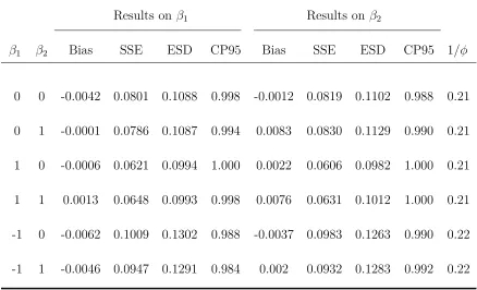
Table 2.1 Estimation of regression parameters for scenario 1 based on 500

simulated data sets from the proposed Bayesian method, para-metric method and Rosen algorithm method. Bias refers to the difference between the average of the 500 point estimates and the true value, ESD refers to the average of the 500 posterior standard deviations, SSE refers to the sample standard devia-tion of the 500 point estimates, and CP95 is the 95% coverage

probability. . . 29

Table 2.2 Estimation of regression parameters for scenario 2 based on 500

simulated data sets from the proposed Bayesian method, para-metric method and Rosen algorithm method. Bias refers to the difference between the average of the 500 point estimates and the true value, ESD refers to the average of the 500 posterior standard deviations, SSE refers to the sample standard devia-tion of the 500 point estimates, and CP95 is the 95% coverage

probability. . . 30

Table 2.3 Comparison MSE of baseline mean functions for differentβamong

the proposed, parametric and Rosen methods for scenarios 1 and 2 35

Table 2.4 The results from three different methods: proposed method,

Rosen method and paramatric method for bladder tumor can-cer data. Variables: X1 and X2 represent the number and the largest size of bladder tumors at beginning of the trial, respec-tively. X3 and X4 are indicators for pyridoxine pill and thiotepa

installation, respectively. . . 39

Table 2.5 Results about regression parameters for different knots with

(10)

Table 3.1 Estimates of regression parameters for scenario 1, when fitting

model with frailty effect for frailty data . . . 55

the model with frailty effect for frailty data . . . 58

Table 3.3 Types of Misspecification . . . 59

the model with frailty effect for no frailty data . . . 60

the model with frailty effect for no frailty data . . . 61

the model with no frailty effect for frailty data . . . 64

the model with no frailty effect for frailty data . . . 65

Table 3.8 Results about regression parameters for different knots with

de-gree=2 and 3 . . . 68

Table 3.9 The estimates of covariate coefficients for Bladder tumor data

from different methods. WZ method: Wellner and Zhang (2007).

YWH method: Yao, Wang and He (2016) . . . 69

Table 4.1 Estimation of regression parameters for scenario 1 based on

500 simulated data sets withsample size 50from the proposed

Bayesian method in Chapter 2. Bias refers to the difference

between the average of the 500 point estimates and the true value, ESD refers to the average of the 500 posterior standard deviations, SSE refers to the sample standard deviation of the

500 point estimates, and CP95 is the 95% coverage probability . . 72

Table 4.2 Estimation of regression parameters for scenario 2 based on

500 simulated data sets withsample size 50from the proposed

Bayesian method in Chapter 2. Bias refers to the difference

between the average of the 500 point estimates and the true value, ESD refers to the average of the 500 posterior standard deviations, SSE refers to the sample standard deviation of the

(11)

Table 4.3 Estimation of regression parameters forscenario 1based on 500

simulated data setsfor the negative binomial event process.

Bias refers to the difference between the average of the 500 point estimates and the true value, ESD refers to the average of the 500 posterior standard deviations, SSE refers to the sample stan-dard deviation of the 500 point estimates, and CP95 is the 95%

coverage probability . . . 78

simulated data setsfor the negative binomial event process.

Bias refers to the difference between the average of the 500 point estimates and the true value, ESD refers to the average of the 500 posterior standard deviations, SSE refers to the sample stan-dard deviation of the 500 point estimates, and CP95 is the 95%

coverage probability . . . 79

Table 4.5 Estimation of regression parameters byusing the frailty model

approach for scenario 1 based on 500 simulated data sets

under the negative binomial event process. Bias refers to

the difference between the average of the 500 point estimates and the true value, ESD refers to the average of the 500 pos-terior standard deviations, SSE refers to the sample standard deviation of the 500 point estimates, and CP95 is the 95%

cov-erage probability . . . 83

Table 4.6 Estimation of regression parameters byusing the frailty model

approach for scenario 2 based on 500 simulated data sets

under the negative binomial event process. Bias refers to

the difference between the average of the 500 point estimates and the true value, ESD refers to the average of the 500 pos-terior standard deviations, SSE refers to the sample standard deviation of the 500 point estimates, and CP95 is the 95%

cov-erage probability . . . 84

simulated data setswhen the observation times depend on

covariates. Bias refers to the difference between the average of

the 500 point estimates and the true value, ESD refers to the average of the 500 posterior standard deviations, SSE refers to the sample standard deviation of the 500 point estimates, and

(12)

simulated data setswhen the observation times depend on

covariates. Bias refers to the difference between the average of

the 500 point estimates and the true value, ESD refers to the average of the 500 posterior standard deviations, SSE refers to the sample standard deviation of the 500 point estimates, and

CP95 is the 95% coverage probability . . . 88

Table 4.9 Estimation of regression parameters for scenario 1 based on

500 simulated data sets for the informative observation

times. Bias refers to the difference between the average of the

500 point estimates and the true value, ESD refers to the average of the 500 posterior standard deviations, SSE refers to the sample standard deviation of the 500 point estimates, and CP95 is the

95% coverage probability . . . 93

Table 4.10 Estimation of regression parameters for scenario 2 based on

500 simulated data sets for the informative observation

times. Bias refers to the difference between the average of the

500 point estimates and the true value, ESD refers to the average of the 500 posterior standard deviations, SSE refers to the sample standard deviation of the 500 point estimates, and CP95 is the

95% coverage probability . . . 94

Table 4.11 Estimation of regression parameters for scenario 2 using the

frailty model approach based on 500 simulated data sets

under the informative observation process. Bias refers

to the difference between the average of the 500 point estimates and the true value, ESD refers to the average of the 500 posterior standard deviations, SSE refers to the sample standard deviation of the 500 point estimates, and CP95 stands for the 95% coverage

probability . . . 98

Table 4.12 Estimation of regression parameters for scenario 2 using the

frailty model approach based on 500 simulated data sets

under the informative observation process. Bias refers

to the difference between the average of the 500 point estimates and the true value, ESD refers to the average of the 500 posterior standard deviations, SSE refers to the sample standard deviation of the 500 point estimates, and CP95 stands for the 95% coverage

(13)

List of Figures

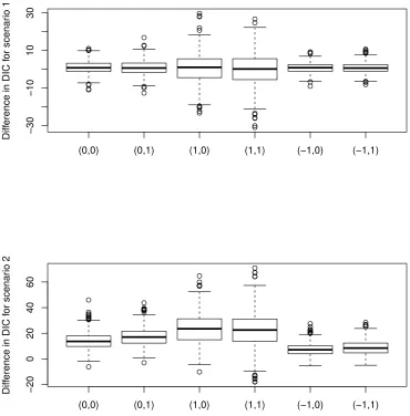
Figure 2.1 Boxplots of DIC difference between degree 2 and degree 3 based

on 500 simulated data sets for the six (β₁,β₂) configurations for

scenario 1 and scenario 2, respectively. . . 27

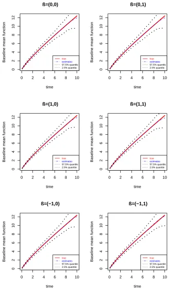
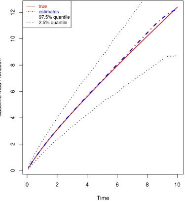
Figure 2.2 Estimates of baseline mean functions for differentβ in scenario 1 32

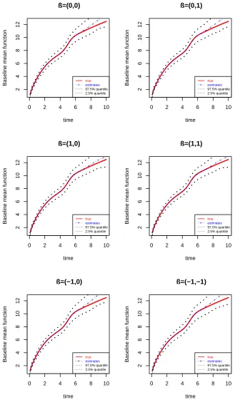
Figure 2.3 Estimates of baseline mean functions for differentβ in scenario 2 33

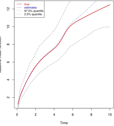
Figure 2.4 Comparison among the true and estimates of cumulative

base-line mean functions among the proposed method, parametric

method and Rosen method for β= (−1,1) for scenario 1 . . . . 36

Figure 2.5 Comparison among the true and estimates of cumulative

base-line mean functions among the proposed method, parametric

method and Rosen method for β= (−1,1) for scenario 2 . . . . 37

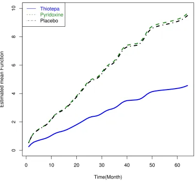
Figure 2.6 Plot for estimated mean function for different treatments . . . 40

Figure 3.1 Estimates of baseline function withβ=(-1,1) for scenario 1 . . . . 56

Figure 3.2 Estimates of baseline function withβ=c(-1,1) for scenario 2 . . . 57

Figure 3.3 Boxplots of DIC differences between frailty and no frailty

mod-els for scenario 1 . . . 62

Figure 3.4 Boxplots of DIC differences between frailty and no frailty

mod-els for scenario 2 . . . 63

Figure 3.5 The estimator of baseline mean function for bladder tumor

ex-ample under the proportional mean model with frailty . . . 66

Figure 3.6 The estimated mean functions for different treatments for

blad-der tumor example unblad-der the proportional mean model with

(14)

Figure 4.1 Estimates of baseline mean functions for differentβinscenario

1 for sample size 50 . . . 74

2 for sample size 50 . . . 75

1 for the negative binomial event process . . . 80

2 for the negative binomial event process . . . 81

1 using the frailty model fitting the data from negative

binomial event process . . . 85

2 using the frailty model fitting the data from negative

binomial event process . . . 86

1 when observation times depend on covariates. . . 89

2 when observation times depend on covariates . . . 90

1 for the informative observation process . . . 96

2 for the informative observation process . . . 97

Figure 4.11 Estimates of baseline mean functions for different β in

sce-nario 1 using the frailty model fitting the data from the

informative observation process . . . 100

Figure 4.12 Estimates of baseline mean functions for different β in

sce-nario 2 using the frailty model fitting the data from the

(15)

Chapter 1 Introduction

1.1 Recurrent Data

1.1.1 Introduction

Recurrent data arise in a lot of areas such as epidemiology, econometrics,

crim-inology, social sciences, reliability and clinic trial study. Recurrent data consist of

times to repeated events for each sample subject. In other words, all these subjects

in the study could experience recurrences of the same event at different times. For

example, in a clinic study, recurrent episodes of a disease in patients appear multiple

times, such as repeated heart attacks, cancer tumors recurrence even after previous

tumors are removed etc.. In a reliability study, when a unit breaks down, it can

be put back into service after being repaired. This situation could occur multiple

times with warranty claims for some particular unit. More examples were given by

Kalbfleisch and Lawless (1981, 1985)[2] [3], Thall and Lachin (1988) [4], and Sun and

Kalbfleisch (1995) [5].

One typical type of recurrent study is the history study of the event of interest.

Since the subjects experience event of interest multiple times, the resulting data are

usually classified as event history data. Generally there are two types of event history

data. One type is the data that can be collected at a continuous time period. We

name this type of data recurrent event data (Byar 1980 [6], Gail 1981 [7], Pepe and

Cai 1993 [8], Lin et al. 2000 [9]), which record the times of all occurrences of events.

(16)

only the number of occurrences of the event between observation times is known. The

exact time of the occurring event of interest is never known. They are often referred

to as panel count data (Kalbfleisch and Lawless 1985 [2], Thall and Lachin 1988 [4],

Sun and Kalbfleisch 1995 [5]).

Recurrent event data are frequently encountered in longitudinal follow-up studies

such as epidemiological and medicinal studies. The observation of the recurrent events

can be terminated at or before the end of the study. For instance, the recurrent events

can have multiple occurrences of hospitalizations, and will be terminated by patients

who loss to follow-up, a fatal event such as death, or the end of the study.

Panel count data are often encountered in periodic follow-up studies. It may

be due to being impractical, too expensive, or not realistic to keep subjects under

continuous observation over the entire study period. The number of observation

times usually varies from one subject to another subject, and the observation times

also vary from subject to subject. In practice, when there is only one observation

time for the event of interest, such as death or onset of disease, the panel count data

are often referred to as current status data (Dinse and Lagakos 1983 [10], Diamond

and McDonald 1992 [11], Jewell and van 1996 [12], Sun and Kalbfleisch 1995 [5]).

Interval censored data can also be viewed as a special case of panel count data.

We are going to mainly focus on panel count data study for this dissertation,

and two examples are presented to further illustrate the basic concepts and general

structures of panel count data.

1.1.2 Examples

(1) Bladder Cancer Tumor Study

Table 1.1 gives a set of panel count data about the bladder cancer study. This

study was conducted by the Veterans Administration Cooperative Urological Research

(17)

superficial bladder tumors when they entered the study. For the first time visit,

the number of the tumors were counted, and the initially largest tumor size was

measured and all the initial tumors were removed transurethrally. Then each patient

was randomly assigned to one of the three treatment groups: placebo, pyridoxine

pill and thiotepa instillation. At each follow-up visit for each patient, the same

procedure was followed: the number of the new tumors was counted, then all of

them transurethrally removed, and then each patient was given the same treatment

as before. Usually a lot of patients had multiple follow-up visits, and had recurrence

tumors through the entire study. In all three treatment groups, the average follow-up

time was about 31 months, but some patients may have been followed as long as

five years. The objective of the study was to determine if the treatments, especially

thiotepa instillation, reduced the recurrence of bladder tumors. The treatment effects

have been analyzed by many authors such as Wei, Lin and Weissfeld (1989) [14],

Wellner and Zhang (2007) [15], Lu, Zhang and Huang (2007, 2009) [16] [17].

(2) National Cooperative Gallstone Study (NCGS)

One of the major interests was to study the safety of the drug chenodiol for the

treatment of cholesterol gallstones. This is a 10-year, multicenter, doubleblinded,

placebo-controlled clinical trial on the use of the natural bile acid chenodeoxycholic

acid, cheno, for the dissolution of cholesterol gallstones (Sun and Zhao 2013 [18]).

There were a total of 916 patients who were assigned one of three treatments:

high-dose (750 mg per day), low-high-dose (375 mg per day), or placebo. One of the primary

objectives of the study was to assess the impact of the treatments on the incidence

of digestive symptoms commonly associated with gallstone disease. The symptoms

could be nausea, vomiting, dyspepsia etc. For example, episodes of nausea vomiting

was viewed as a very common symptom associated with gallstone diseases and very

important for the investigators to determine whether there exists a significant

(18)

Table 1.1: Numbers of new tumors at each visit for selected subjects with placebo treatment and Thiotepa treatment

Patient Start Numbers of new tumors at following months

ID Size 0-10 11 -20 21-30

1 3 1 0 . . . .

2 1 2 0 . . 0 . . 0 . . . .

12 3 3 . . 1 . . 0 . . 1 0 . . 0 . 0 . 0 . . 0 8 . 0 . . . .

17 4 1 . 4 . . . 0 . . . 8 . . . .

23 5 1 . 4 . . . 0 . . . 2 . . . 4 0 . . . . 0 .

Thiotepa group

48 3 1 0 . . . .

50 1 8 . . . . 8 . . . .

79 4 1 0 0 0 0 0 0 0 0 0 0 0 0 0 0 0 0 0 0 0 0 0 0 0 0 0 0 0 0

81 1 4 . . . 1 . . . 0 . . . . 0 . . . 0 . . 1 . . . .

85 3 1 0 0 0 0 0 0 0 0 0 0 0 0 0 0 0 0 . 0 . 0 0 0 . 0 0 0 0 0 .

The symptoms were observed shortly after they achieved maximal dose, since it was

believed that any treatment had an effect right after taking the doses, and the effect

might later begin to dissipate. During the study, the patients were scheduled to

re-turn for clinic observations for each follow-up visit. For the first year, they were asked

to return at 1, 2, 3, 6, 9, and 12 months, and to report the total number of each type

of symptom that had occurred between successive visits such as the number of the

incidences of nausea. However, the actual visit times varied from patient to patient.

For example, some patients may visit more often at the first half a year than the later

half a year, some patients may drop off the study. Table 1.2 is a selected data subset

which has visit times in weeks and observed counts of episodes of nausea for patients

with floating gallstones. The whole data set has been studied in many references (Wei

(19)

Table 1.2: Visit times in weeks and observed counts of episodes of nausea for some patients with floating gallstones in the National Cooperation Gallstone Study

Patient Visit times and episodes of nausea

ID t1 N1 t2 N2 t3 N3 t4 N4 t5 N5 t6 N6 t7 N7 t8 N8 t9 N9

High-dose chemo group

1 4 0 8 0 13 0 26 0 38 0 51 0 69 0 . . . . 10 4 0 9 0 13 0 17 0 22 0 26 0 38 0 43 0 62 0 32 3 1 9 3 13 0 26 0 38 0 52 0 70 0 . . . . 50 3 0 8 0 13 0 25 8 37 20 53 0 73 0 . .

Placebo group

64 4 0 8 0 12 0 25 0 38 0 52 0 68 0 . . . . 70 4 0 8 0 13 0 24 0 37 0 50 0 67 0 . . . . 103 4 3 . . . . 111 4 0 9 0 14 0 25 0 . . . .

1.2 Analysis of Panel Count Data

As we know the study subjects in panel count data are monitored at discrete time

points, and the observable information is the event counts for each subject

corre-sponding to the time interval between two adjacent time points, but the exact times

of the event is not observable. Moreover, the observation times for each subject are

not often the same, which makes the counts among subjects not directly comparable.

Based on the incomplete and unbalanced nature of observed information, to

ana-lyze recurrent event data, it is common and convenient to characterize the occurrences

of recurrent events by counting process (Andersen et al. 1982 [21]) and to model the

intensity process of the counting process. On the other hand, for the analysis of panel

count data, it is usually more convenient to work directly on the mean function of

the counting processes conditional on covariate processes (details in Sun and Zhao

(20)

parametric Poisson processes or mixed parametric Poisson processes. For example,

Lawless (1987) [22] provided a thorough parametric analysis of the proportional

in-tensity Poisson process model, where subject-specific gamma random effects and a

Weibull baseline intensity function were assumed. Thall (1988) [4] developed some

regression approaches for mixed Poisson. There are quite a few methods for panel

count data with the assumption of nonhomegeneous Poisson process. For example,

Wellner and Zhang (2000) [23] studied nonparametric maximum pseudolikelihood and

nonparametric maximum likelihood estimators based on a nonhomogeneous Poisson

process. They showed that the maximum pseudolikelihood estimator was exactly the

one proposed by Sun and Kalbfleisch (1995) [5]. They also discussed the asymptotic

properties of the maximum pseudolikelihood and maximum likelihood estimators.

Compared with maximum pseudolikelihood estimator, the maximum likelihood

esti-mator is much more efficient, but its computation is more difficult.

Many investigators have studied spline estimation of a hazard function for panel

count data. Whittemore and Keller (1986) [24] used step functions and linear splines

to obtain non-parametric estimates of the baseline hazard function. Etezadi-Amoli

and Ciampi (1987) [25] applied quadratic splines to obtain smoother estimates.

Rosen-berg (1995) [26] modeled the hazard function as a linear combination of cubic-splines

and obtained maximum likelihood estimates. Lu, Zhang and Huang (2007, 2009)

[16] [17] proposed nonparametric spline likelihood-based estimators using monotone

polynomial splines and semiparametric monotone B-splines, respectively.

In some cases, panel count data may show a higher incidence of zero counts than

expected if the data were Poisson distributed. Zero-inflated Poisson regression

mod-els are a useful class of modmod-els for modeling such data, but parameter estimates

may be seriously biased if the nonzero counts are overdispersed in relation to the

Poisson distribution. Ridout et al. (2001) provided zero-inflated negative binomial

(21)

testing zero-inflated Poisson regression models against zero-inflated negative binomial

alternatives.

In the rest of these sections, we provide a review about counting process, the mean

cumulative function and regression models for panel count data, respectively.

1.3 Counting Process

We know that panel count data study is a special type of event history study.

The observation counts are inevitably involved in the study. The counting processes

have been playing an essential and important role in the development of statistical

models and inferential procedures for this kind of event history analysis. Especially,

it is widely applied in analyzing panel count data. Some of the early and

signifi-cant contributions to this were provided by Aalen (1975, 1978) [27] [28], Andersen

and Borgan (1985) [29], and Liaw (1995) [30]. They established the connection

be-tween the counting process and the event history analysis, and provided the theory of

counting processes and a general framework for event history analysis. In particular,

Andersen and Gill (1982) [21] proposed the Cox type intensity model for counting

processes, developed the partial likelihood estimation procedure for regression

param-eters, and established the large sample theory for the resulting estimators. Andersen

et al. (1993) [31] gave more details about counting processes.

Let (Ω,F,P) be a probability space and T = [0, τ) a continuous time interval,

where τ is a given terminal time, 0 < τ ≤ ∞. A stochastic process X is a family of

random variables {X(t) : t ∈ T}. A filtration or history {Ft : t ∈ T} is an

increas-ing right-continuous family of sub σ-algebras of F, it contains all the information

generated by the stochastic process X on [0, t]. If X(t) is Ft-measurable for every

t ∈ T, then the stochastic process X is said to be adapted to the filtration. If X(t)

is known given the history Ft− generated by {X(s) : 0≤ s < t}, then the stochastic

(22)

count-ing process is a stochastic process {N(t) : t ≥ 0} with almost surely such that the

path is right-continuous with probability one, piecewise constant, and has only jump

discontinuities with jumps of size plus 1.

Usually we use the intensity to model a counting process, it could be defined by

P{N(t+dt)−N(t) = 1|Ft}=λ(t)dt+o(dt)

and

P{N(t+dt)−N(t)≥2|Ft}=o(dt)

with λ(t) being a left-continuous function. If the counting process is Poisson process

N(t), based on the definition above, we can see that the Poisson process N(t) only

has at most one jump over a small time interval and does not depend on its history.

A non-homogeneous Poisson process ( Karlin and Taylor 1981 [32]) is a very common

and widely applied special counting process. If λ(t) is a constant, the process is

usually called a homogeneous Poisson process. For a Poisson process {N(t) : t ≥0}

at each t, we have thatN(t) follows the Poisson distribution.

Among all counting processes, the Poisson process {N(t) : t ≥ 0} as the most

commonly used one has been shown a large contribution to queuing theory, risk

theory and a lot of types of the application in model building area for our real life.

There are a lot of examples of phenomena that can be modeled by Poisson processes

with many kinds of ways. In traffic processes in networks such as computer systems,

machine repair shops etc, traffic flows within the network are postulated as Poisson

processes in Melamed (1979) [33]. A compound Poisson process had been used to

model cumulative energy release of main shocks in the Balkan region for Balkan

earthquake sequences by Gospodinov and Rotondi (2001) [34].

Landfalling hurricanes recorded along the U.S. Gulf and Atlantic coasts between

1900 and 2010, and their associated maximum wind speed and damages were studied

by modeling the sequence of nonhomogeneous density functions in Xiao et al. (2015)

(23)

We will discuss and study our models about panel count data based on the

non-homogeneous Poisson process in the following chapters.

1.4 Mean Cumulative Function

Recurrence data consist of the times to any number of repeated events for each

sample unit, for example, times of new bladder tumor observed in patients or times

of repair of warrantied product. Sometimes the data are censored due to different

ends of histories or study. Panel count data contains the counts of repeated events

till particular observation times. After Cox (1972) [36] provided the proportional

hazards model, Lawless and Nadeau (1995) [30] and Lin et al. (2000) [9] described

proportional rates and proportional means regression models for recurrence data.

The mean cumulative function for the number of the events usually contains the

information of interest in the analysis of panel count data. Actually in many cases,

the mean function is of more interest and modeling it directly is desirable. And we

know that the aim of fitting a Cox model to time-to-event data is to estimate the

effect of covariates on baseline hazard function, the aim of fitting proportional mean

models is very smaller to it, i.e, the aim is to estimate the effect of covariates on

the baseline mean cumulative function. Since the baseline hazard function is not

itself estimated, there is no big risk of misspecifying the baseline distribution. how to

construct or define the baseline function depends on one’s perspective on what else

effects will be considered in the models, and depends on how to combine it with the

covariates in practice in order to get the ideal results in study.

The proportional mean model is as follows:

U(t|X) =E{N(t)|X}=U0(t)exp(X0β), (1.1)

where {N(t), t > 0} is a counting process, X is a vector of invariant covariates.

(24)

nondecreasing function, β is a p x 1 vector of the regression coefficients.

In practice, if we obtain the mean cumulative function, it is easy to get information

not only from the quantity of it, but also from the plot visually. For example, by some

timet, whether the rate of occurrence of events is increasing, decreasing, or constant,

and whether several groups differ significantly in expected number of events can be

explained by the mean cumulative function. In Chapters 2, 3 and 4, we will adopt

the proportional mean models to analyze the panel count data.

1.4.1 I-Splines

A spline is a real function which was introduced by Schoenberg (1964) [37] in

connection with smooth, piecewise polynomial approximation. It has been developed

from different purposes in terms of B-splines, G-splines, smoothing splines, I-splines,

etc.. In the following, we will briefly introduce how to construct splines, and then

mainly focus on introduce monotone I-splines, which will be used as an approximation

for the baseline mean cumulative function in our models.

Let’s start with M-splines. First, two crucial components are needed in order to

construct M-splines. One is the degree of the polynomial, and the other is the knots

which partition an interval into a number of subintervals. Let’s choose the degree d

and set up m interior knotsξ1 <· · ·< ξm within the interval [a, b].

M-spline can be written as the formf =Pn

i=1ciMi, whereMi is the basis functions

constructed by the following recursive formulas, andci is coefficient of basis function.

Set s1 = a, s2 =ξ1,· · · , sm+1 = ξm, and sm+2 = b, then for i = 1,2, . . . , m+ 1, and

d= 1,

Ml(t|1) =

    

   

1

sl+1−sl, sl ≤t < sl+1,

0, otherwise;

for d ≥ 2, let s1 = · · · = sd = a, sd+1 = ξ1,· · · , sd+m = ξm, and sm+d+1 = · · · =

(25)

Ml(t|d) =         

[(t−sl)Ml(t|d−1)+(sl+d−t)Ml+1(t|d−1)]

(k−1)(sl+d−sl) , sl ≤t < sl+d,

0, otherwise.

Note that eachMl(·|d) is a piecewise polynomial with nonzero only within [sl, sl+d)

forl = 1, . . . , m+d, andR

Ml(x)dx= 1. The reason is that this partition points only

affect the change of the coefficient ai within this interval. Also we can see that the

individual polynomials always have the same degree and connect smoothly at join

points (knots).

Based on M-splines, one can construct two specific splines: B-spline and I-splines.

The B-splines can be constructed in the form: f = Pq

i=0ciBi, where Bi is the basis

functions constructed by Bi = (ti+k−ti)Mi/d. q needs to be specified. The I-splines

are the integrated functions of M-splines defined as follows:

Il(t|d) =

Z t

L

Ml(u|d)du. (1.2)

Specifically, for t ∈[sj, sj+1). Il(t|d) takes the following form,

Il(t|d) =

                  

1, l < j−d+ 1,

Pj

h=1(sh+d+1−sh)

Mh(t|d+1)

d+1 j −d+ 1≤l ≤j,

0, l > j.

(1.3)

The I-splines can be constructed in the form:

g(t) =

k

X

i=0

ciIi(t),

where Ii(t) is the basis functions as (1.3), I0(t) = 1 for any t. ci is coefficient of

basis function, it has to be nonnegative eo ensure thatg is nondecreasing. Similar to

B-splines, two crucial components are needed to specify the I spline basis functions:

the knots and the degree. The placement of the knots determines the shape, and

(26)

are totally determined after the knots and the degree are specified. The number of

spline basis functions k equals the number m of interior knots plus the degree d of

the splines. We refer to Ramsay (1988) [1] where more details about I splines were

provided.

In general, the shape of a spline function is robust to knot placement. We will

discuss more about how to choose the number of the interior knots and the degree of

the splines in the following chapter.

1.5 Deviance Information Criterion

In Bayesian method study, The deviance information criterion, Akaike

informa-tion criterion and Bayesian informainforma-tion criterion are widely used to get deviance

information in model selections. There are many literitures that can be found about

their application. Comparative performance of Bayesian and AIC-based measures

of phylogenetic model certainty was studied in Alfaro and Huelsenbeck (2006) [38].

Wang (2009) [39] developed a generalized Bayesian information criterion for regression

model selection. Ando (2007) [40] discussed about Bayesian predictive information

criterion for the evaluation of hierarchical Bayesian and empirical Bayes models.

Er-ven and Grunwald (2012) [41] proposed a predictive approach to adaptive estimation

with an application to the AIC-BIC dilemma.

The deviance information criterion (DIC) is a hierarchical modeling generalization

of the Akaike information criterion (AIC) and Bayesian information criterion (BIC).

It is very similar to AIC and BIC, since it is also an asymptotic approximation as

the sample size becomes large. Claeskens and Hjort (2008) [42] showed that the

DIC is large-sample equivalent to the natural model-robust version of the AIC. It is

particularly useful in Bayesian model selection problems, especially, for some model

selections, and the posterior distributions can be easily obtained by Markov chain

(27)

Define the deviance asD(θ) =−2log(p(x|θ))+C,wherexis the data,θis unknown

parameter of the model and p(x|θ) is the likelihood function. C is a constant, it will

not be necessary to know, because it will be cancelled out in all the calculations when

comparing different models.The expectation ¯D = Eθ[D(θ)] is a measure of how well

the model fits the data; the smaller it is, the better the model fits.

In order to get DIC, some calculations have to be made. There are two ways

that can be considered for getting the effective number of parameters included in the

model. The first way, as described in Spiegelhalter et al. (2002) [43], is to calculate

pD = ¯D−D(¯θ),

where ¯θ is the expectation of θ.

The second one, as described in Gelman et al. (2004) [44] is to get pD by calculating

the varivances as follows,

pD =pV =

1

2var (d D(θ)).

The larger the effective number of parameters is, the easier it is for the model to fit

the data, and so the deviance needs to be penalized. The formula for calculating the

deviance information criterion is

DIC =pD+ ¯D,

or equivalent to

DIC =D(¯θ) + 2pD.

or

DIC = 2 ¯D−D(¯θ). (1.4)

The advantage of DIC over other criteria in the case of Bayesian model selections

(28)

chain Monte Carlo simulation. AIC and BIC require calculating the likelihood at its

maximum over θ,which is not readily available from the MCMC simulation. But to

calculate DIC, as long as one can find the likelihood function, then simply compute

¯

Das the average of D(θ) over the samples of θ,and D(¯θ) as the value of D evaluated

at the average of the samples of θ, then just take some calculations by the formula

of getting the DIC. In the following chapters, DIC is used as one of criteria for the

(29)

Chapter 2 Bayesian Semiparametric Proportional Mean

Model for Panel Count Data

2.1 Introduction

Panel count data often arise in epidemiological studies, industry reliability,

long-term clinic trials, and animal experiments. Kalbfleisch and Lawless, Gaver and

OMuircheataigh, Thall and Lachin, Thall, Sun and Kalbfleisch, and Wellner and

Zhang etc. have been studying in the area a lot. By panel count data, it means

that it is not feasible or not practical to continuously observe each subject, but the

event of interests has a property of recurrence, and the study subjects are monitored

periodically. For such studies, since the subjects are not under continuous

monitor-ing, the exact time of each recurrent event is not observed but the count of such

events between any two adjacent observation times is known. For example, in the

bladder cancer study (Byar 1980 [6]), the famous example in the literature of panel

count data, the number of new tumors is counted for each follow-up visit after the

old tumors are removed at each visit. The observation times, i.e., the times at clinic

visits, are different for different subjects, which makes the counts among subjects not

directly comparable. Panel count data often can be considered as a special type of

longitudinal data with a count response variable (sun and Zhao 2016 [45]).

Poisson models are commonly used for analyzing count data. However, the regular

Poisson models ignore the longitudinal property of panel count data. To incorporate

(30)

a counting process is usually assumed and the observed counts are assumed to be

collected at discrete time points from the counting process. Earlier research on panel

count data focused on the estimation of the mean function of the counting process

when there are no covarites. For example, Sun and Kalbfleisch (1995) [5] applied

the isotopic regression method and proposed a nonparametric estimate of the mean

function. Wellner and Zhang (2000) [23] proposed both a nonparametric

pseudo-maximum likelihood estimator and the full pseudo-maximum likelihood estimator of the

mean function based on a non-homogeneous Poisson process. Hua and Zhang [46]

discussed a semiparametric analysis of panel count data within the framework of

GEE, assuming the proportional mean model as in Wellner and Zhang (2007) [15]

and Lu et al. (2009) [17].

Spline techniques have been widely used to approximate unknown functions in

statistics literature. For modeling panel count data, Lu et al. (2007) [16] adopted

monotone B-splines to model the mean function in the nonparametric setting and

showed that their spline likelihood estimators outperformed the estimators proposed

by Wellner and Zhang (2000) [23] in terms of convergence rate and finite sample

performance. Lu et al. (2009) [17] then extended the work of Lu et al. (2007)

[16] to the regression setting and used the monotone cubic B-splines to approximate

the logarithm baseline mean function. Hua and Zhang (2012) [46] adopted the same

spline specification and obtained the estimates of the regression parameters and spline

coefficients by projecting the GEE estimates into a feasible domain under the

pro-portional mean model. In this chapter, we assume the propro-portional mean model for

the panel count data and use monotone I-splines (Ramsay 1988 [1]) to model the

baseline mean function. Our spline coefficients only require being nonnegative to

ensure the monotonicity of the baseline mean cumulative function. Furthermore, the

monotone I-spline specification and the nonnegative restriction naturally fit in the

(31)

Compared to the flourish work in the frequentest literature, Bayesian approaches for

panel count data seem to be very limited. Chib and Greenberg (1998) [47] conducted

Poisson regression on correlated count data with the correlation among the counts

modeled by multivariate normal latent effects. Sinha and Maiti (2004) [48] proposed

a Bayesian approach for the analysis of panel count data with a dependent

termi-nation following a discreet Cox model. However, Sinha and Maiti (2004) [48] made

restrictive assumptions that the observation times are the same for three all subjects

and that the termination times only take values of the observations times.

In many applications, the effects of covariates on the panel count are of interest.

Wellner and Zhang (2007) [15] extended their two likelihood-based methods (Wellner

and Zhang 2000 [23]) by incorporating covariates under a proportional mean

regres-sion model (2.1) associated with the assumption of a non-homogeneous Poisson

pro-cess.Their methods are shown to be robust against misspecification of the underlying

counting process, as long as the proportional mean model 2.1 holds. The likelihood

estimator is more efficient than the pseudolikelihood estimator, but its computation

is very intensive. And also it can be very inefficient when the distribution of the

number of observations times is heavily tailed, which is shown in an ex-ample given

by Wellner, Zhang and Liu (2004) [49]. In Wellner and Zhang (2007) [15], a

substan-tial amount of computation was required in the bootstrap semiparametric inference

procedure. Therefore it is desirable to develop some methods that not only maintain

good statistical properties, but also are less computationally intensive.

Generally, various methods of panel count data and recurrent timed data were

developed with mainly putting high emphasis on partially specified models. In suck

work, the models and associated inferential procedures depend on the particular

un-derlying inferential objective. These can be of the following four types as mentioned

in Sinha and Maiti (2004) [48]. (1) Inference about the event count under the

(32)

time; (2) Marginal inference about event count unconditional on past history of event

; (3) Inference about observation time given the covariate information or the history

of event count; and (4) Inference about the termination modulation process (Ghosh

and Lin 2003 [50]). For example, Sinha and Maiti (2004) [48] developed and analyzed

a fully specified stochastic model of the joint distribution of the nonfatal events and

the termination time through the likelihood of their model and associated Bayesian

methods for analysis under the assumption of a compound nonhomogeneous Poisson

process.

In this chapter, we provide a very flexible Bayesian approach for analyzing panel

count data, where the dependent termination is not considered, but the number and

the sequence of observation times are allowed to be different across subjects. The

proposed Bayesian approach provides an accurate estimation of both the regression

parameters and the baseline mean function. Beside, our approach is computationally

efficient and easy to implement.

The remainder of this chapter is organized as follows. First the details of data

structure are given in Section 2.2. The specification of monotone splines is presented

in Section 2.3. Section 2.4 augments the likelihood function under the Poisson process

assumption about the panel count of interest. Prior specification and an efficient

algorithm of Gibbs sampler are presented in Section 2.5. Section 2.6 presents the

simulation results of the estimates of regression parameters and the estimates of

baseline function for two scenarios, respectively. Model selections in terms of the

number of knots and degrees of the splines are discussed in Section 2.6 as well. The

comparison about the estimates of regression parameters and baseline mean function

is provided with two other existing methods in Section 2.6.4. A real data set is

illustrated by our proposed method in Section 2.7. Finally, the conclusion and some

(33)

2.2 Notation and Model

Panel count data is to record the counts of recurrent events between every two

visit times for each subject. In practice, it can be treated as cluster data, and all the

observations from the same subject can be thought of as a cluster. Suppose we have

n independent subjects (clusters) for a set of panel count data, for each subjecti, the

data are collected at Ki random time points 0 < ti1 < ti2 < . . . < tiKi, where Ki is

a random variable that takes positive integer values, and tiKi is the last observation

time of subject i. DenoteNi(t) as the number of events observed before and at time

t for subject i, then Ni(t) is a counting process for cluster i. So the panel counts for

the counting process Ni(t) are Ni = (Ni(ti1), Ni(ti2), . . . , Ni(tiKi).

Without loss of generality, we assume initial counts Ni(ti0) = 0 for i= 1, . . . , n.

We have the whole set of observed panel count data denoted byDi ={tij, Ni(tij), Xi,

for i = 1, . . . , n, j = 1, . . . , Ki}, where Xi is a p-dimensional vector of covariates.

Denote D = (D1, . . . ,Dn). Assume that the counting process Ni(·) is independent of

the number Ki of the observation times and the sequence of the observation times

ti1, ti2, . . . , tiKi. Then we have the following proportional mean model:

E(Ni(t)|Xi) =U0(t)exp(Xi0β), (2.1)

for i = 1, . . . , n, where U0(t) is the baseline mean cumulative function and β is a

vector of covariate effects. Model (2.1) has been widely studied in semiparametric or

parametric analysis, for instance, in Balshaw and Dean (2002) [51], Huang, Wang and

Zhang (2006) [52], Lu, Zhang and Huang (2007) [16], and Wellner and Zhang (2007)

[15]. Let Zij be the count of recurrences within the jth time interval [ti,j−1, tij), then

Zij will be written asZij =Ni(tij)−Ni(ti,j−1), for j = 1, . . . , Ki. In this chapter, we

assume thatNi(t) follows a nonhomogeneous Poisson process, thenZij independently

follows the Poisson distribution as follows:

Zij|Xi ∼ P

n

U0(tij)−U0(tij−1) o

exp(X_i0β) !

(34)

The whole set of observed data can also be denoted by D = {tij, Zij, Xi, for i =

1, . . . , n, j = 1, . . . , Ki}.

2.3 Modeling U0(t) with Monotone I- splines

Monotone I-splines (Ramsay 1988 [1]) have recently been widely applied in

semi-parametric survival models such as in Wang and Dunson (2011) [53], Wu et al. (2012)

[54], and Lin et al. (2015) [55]. Monotone I-splines are often adopted to approximate

unknown nonnegative and nondecreasing functions. In this dissertation, monotone

I-splines (Ramsay 1988 [1]) are also adopted to approximate the unknown nonnegative

and nondecreasing function U0(t). The formula is as follows:

U0(t) =

L

X

l=1

rlIl(t|d), (2.3)

whereIl(·|d) i monotone I-spline basis function with degree d and each is

nondecreas-ing from 0 to 1, andrls are nonnegative spline coefficients to ensure the monotonicity

of the nonnegative function U0(t). The detailed formulation of the basis function

Il(·|d) is provided in Chapter 1, and more details can be found in Ramsay (1988)

[1] and Lin et al. (2015) [55]. The degree d and the knot placement are two crucial

components to determine the basis functions. The numberLof the basis functions is

equal to the degreed plus the numberm of interior knots and plus 1. In general, the

degreed controls the smoothness of the splines and taking degree as 2 or 3 is usually

enough to ensure the smoothness. The placement of knots controls the shapes of

the basis splines, and as a consequence, they effect the shape of the final fitted

func-tion. Usually, the more knots in a region, the greater the flexibility of the function

in that region; the more data points between a pair of knots, the better fitted the

curve in that interval (Lawless 1987 [22]). According to Cai et al. (2011) [56] and

Wang and Dunson (2011) [53], in general, using 10 to 30 knots can provide adequate

(35)

equally-spaced knots or quantile-based knots, which depends on data itself.

More-over, Bayesian model comparison criteria such as the deviance information criterion

(DIC) (Spiegelhalter et al. 2002 [43]) and log pseudo marginal likelihood (LPML)

(Ibrahim et al. 2001 [57]) would also be useful to help with selection of the best setup

of the degree and the number of knots.

In this chapter, we use the comparison criterion of deviance information criterion

( DIC) (Spiegelhalter et al. 2002 [43]) to determine the best setup of I-splines in the

simulation part in Section 2.6 and the real data analysis in Section 2.7.

2.4 Likelihood Augmentation with Poisson Latent Variables

Since{Ni(t), t >0}follows a non-homogeneous Poisson process, andZij is defined

as the count difference between time pointsti,j−1andti,j,i.e.,Zij =Ni(tij)−Ni(ti,j−1),

for i = 1, . . . , n, and j = 1, . . . , Ki. Based on the properties of a nonhomogenous

Poisson process, Zij independently follows Poisson distribution conditionally on the

covariates Xi,

Zij|Xi ∼ P

n

U0(tij)−U0(tij−1) o

exp(X_i0β) !

.

Under the nonhomogenous Poisson process assumption (givenX), the observed

like-lihood function is

L(θ|D) =

n

Y

i=1

Ki

Y

j=1

exp "

−nU0(tij)−U0(tij−1) o

exp(X_i0β) #

" n

U0(tij)−U0(tij−1) o

exp(X_i0β) #Zij,

Zij!, (2.4)

whereθ is a vector of all unknown parameters including β and r= (r1, . . . , rL).Note

that for the notation convenience, we omit degree din the basis functions. Under the

monotone I-spline approximation to U0(t), U0(t) = PLl=1rlIl(t), then the likelihood

(36)

L(θ|D) = n Y i=1 Ki Y j=1 exp " −n L X l=1

rlIl(tij)− L

X

l=1

rlIl(tij−1) o

exp(X_i0β) #

×

" n_XL

l=1

rlIl(tij)− L

X

l=1

rlIl(tij−1) o

exp(X_i0β) #Zij,

Zij!. (2.5)

This likelihood function is very complex, especially for the term

" nXL

l=1

rlIl(tij)− L

X

l=1

rlIl(tij−1) o

exp(X_i0β) #Zij

. (2.6)

This term makes sampling eachrl very difficult. To facilitate the computation,

inde-pendent Poisson latent variables Zij1, . . . , ZijL are introduced to decompose Zij such

that Zij = PLl=1Zijl. By the additivity property of Poisson random variable, each

single Zijl independently follows a Poisson distribution as follows:

Zijl|Xi ∼ P

n

rlIl(tij)−rlIl(tij−1) o

exp(X_i0β) !

,

for i= 1, . . . , n, j = 1, . . . , Ki,and l= 1, . . . , L.

Then the augmented likelihood function with Z_ijl0 s is

Laug = n Y i=1 Ki Y j=1 L Y l=1 exp "

−nrlIl(tij)−rlIl(tij−1) o

exp(X_i0β) #

×

" n

rlIl(tij)−rlIl(tij−1) o

exp(X_i0β) #Zijl,

Zijl!. (2.7)

The augmented likelihood function (2.7) gets rid of all the summation signs in the

term of (2.6), and adds another of multiplication in front of the whole expression of

the likelihood function. As a result, each parameter rl can be easily factored out,

which is much helpful for obtaining their full conditional distributions and ease the

(37)

2.5 Prior Specification and Posterior Computation

For Bayesian posterior computation, we need to assign priors for the unknown

parameters β and rl. For βm, m = 1, . . . , p, we assign conventional independent

vague normal priors with mean zero and large varianceσ2

m such as 100. This leads to

a log-concave full conditional posterior distribution for eachβm, and can be sampled

easily using the adaptive rejection sampling (ARS) (Gilks and Wild 1992 [58]). For

rl, l= 1, . . . , L,we assign independent exponential exp(λ) priors with a Gamma hyper

prior G(aλ, bλ) for λ with mean aλ/bλ and variance aλ/b2λ. This prior specification is

appealing from the computational perspective because it leads to conjugate forms

for each of the conditional posterior distributions of rl0s and λ. Theoretically, such a

prior specification is closely related to Bayesian Lasso (Park and Casella 2008 [59])

and is equivalent to the penalized likelihood approach withL1 penalty on those spline

coefficients, in whichλserves as a tuning parameter. This prior specification penalizes

large values of the coefficients rls and functions to shrink the coefficients of those

unnecessary spline bases towards zero. This property allows us to use many knots

to provide adequate modeling flexibility but does not cause over-fitting problems. In

the penalized likelihood approach, selecting a properλvalue requires much additional

work using cross-validation method. In contrast, our approach treats λ as random

and assigns the Gamma hyper prior for λ to allow for automatic tuning with much

less computational efforts. Our simulations show that our approach is very robust to

the choice of the hyperparameters in the Gamma hyper prior of λ. Here we choose

aλ = 1 and bλ = 1.

Gibbs sampling (Geman and Geman 1984 [60], Gelfand and Smith 1990 [61]) is

one of the most popular MCMC algorithm (Casella and robert 2004 [62]) for

sam-pling the joint posterior distribution. We adopt Gibbs samsam-pling for samsam-pling the

joint posterior distribution. Typically, it requires sampling all the unknown

(38)

the MCMC chains converge, the samples can be considered from the target joint

pos-terior distribution. Based on the augmented likelihood function (2.7) and the above

specified prior distributions, the Gibbs sampler is derived with the four sets of the

full conditionals as below:

1. Sample rl from a Gamma distributions G(Al, Bl), forl = 1, . . . , L, where

Al = n X i=1 Ki X j=1

Zijl+ 1,

Bl = n

X

i=1

n

Il(tiKi)−Il(ti0)

o

exp(X_i0β) +λ.

2. Sample βm by using the adaptive rejection sampling (ARS) (Gilks and Wild 1992

[58]) method, form = 1, . . . , p, because the full conditional distribution of each

βm is proportional to

exp " − n X i=1 L X l=1 rl n

Il(tiKi)−Il(ti0)

o

exp(X_i0β)

+ n X i=1 Ki X j=1

(X_i0β)Zij −βm2/(2σ

2₎

#

,

which is a log-concave function of βm. This readily available software program

for the adaptive rejection sampling method (Gilks and Wild 1992 [58]) has been

widely used to sample from these log-concave densities such as Sinha and Maiti

(2004) [48], Yao and Wang (2016) [63] etc.

3. Sample Zijl, for i= 1, . . . , n, j = 1, . . . , Ki and l = 1, . . . , L. It is from a

multino-mial distribution with parameters Zij and Pij, denoted by M(Zij,Pij), where

Pij = (pij1,· · · , pijL) with PLl=1pijl = 1, and

pijl=

rl{Il(tij)−Il(ti,j−1)} PL

l=1rl{Il(tij)−Il(ti,j−1)}

,

(39)

4. Sample λ from a Gamma distribution G(aλ+L, bλ+PLl=1rl).

The above developed Gibbs sampler is very efficient and easy to implement, because

all the full conditional distributions either have closed forms or they are log-concave.

2.6 Simulation Studies

2.6.1 Data Generation

An extensive simulation study is conducted to evaluate the proposed approach.

Data sets are generated as follows. The event count of each subject i is assumed to

follow a nonhomogeneous Poisson process with the mean function modeled as (2.1),

E(Ni(t)|Xi) =U0(t)exp(Xi0β),

where covariatesXi = (Xi1, Xi2) withXi1generated from Bernoulli(0.5) andXi2from

N(0,0.5). Each subject is repeatedly observed at a random number Poisson(6) + 1

of times and the counts of event are collected, and the gap times between any two

adjacent observation times are drawn from an exponential distribution with mean 0.5.

We set up the true regression coefficients β1 = 0,1, or −1 and β2 = 0 or 1, resulting

in 6 combinations of regression coefficients. For the true baseline mean function U0,

we choose two scenarios:

Scenario 1, U0(t) =t+ log(1 +t), which is approximately linear.

Scenario 2, U0(t) = 0.5Φ(t,1,1) + 0.5Φ(t,5,0.5) +t0.5, where Φ(·) is the cumulative

distribution function of the standard normal distribution. It is clear that for this

scenario, U0(t) is curvilinear and has multiple reflection points.

We totally perform 12 simulation setups. For each setup, 500 data sets are

sim-ulated and each data set has 150 subjects. The proposed Gibbs sampler in Section

5 is implemented for each simulated data set. All the summarized results are based

on 5000 iterations of the Gibbs samples after discarding the first 1000 iterations as a

The Effect of Professional Development on Middle School Teachers' Technology Integration: An Action Research Study

University of South Carolina

Scholar Commons

Bayesian Semiparametric Methods for Analyzing

Panel Count Data

Jianhong Wang

Acknowledgments

Abstract

Table of Contents

List of Tables

List of Figures

Chapter 1

Introduction

Chapter 2

Bayesian Semiparametric Proportional Mean

Model for Panel Count Data