Machine Learning Classification of Interplanetary Coronal Mass Ejections Using Satellite Accelerometers

(1)

Western University Western University

Scholarship@Western

Electronic Thesis and Dissertation Repository

10-1-2019 2:45 PM

Machine Learning Classification of Interplanetary Coronal Mass

Ejections Using Satellite Accelerometers

Kelsey Doerksen

The University of Western Ontario

Supervisor

Dr. Kenneth McIsaac

The University of Western Ontario Co-Supervisor Dr. Jayshri Sabarinathan

The University of Western Ontario

Graduate Program in Electrical and Computer Engineering

A thesis submitted in partial fulfillment of the requirements for the degree in Master of Engineering Science

Follow this and additional works at: https://ir.lib.uwo.ca/etd

Part of the Aerospace Engineering Commons, and the Electrical and Computer Engineering Commons

Recommended Citation Recommended Citation

Doerksen, Kelsey, "Machine Learning Classification of Interplanetary Coronal Mass Ejections Using Satellite Accelerometers" (2019). Electronic Thesis and Dissertation Repository. 6715.

https://ir.lib.uwo.ca/etd/6715

This Dissertation/Thesis is brought to you for free and open access by Scholarship@Western. It has been accepted for inclusion in Electronic Thesis and Dissertation Repository by an authorized administrator of

(2)

Space weather phenomena is a complex area of research as there are many different variables and signatures that are used to identify the occurrence of solar storms and Interplanetary Coro-nal Mass Ejections (ICMEs), with inconsistencies between databases and solar storm cata-logues. The identification of space weather events is important from a satellite operation point of view, as strong geomagnetic storms can cause orbit perturbations to satellites in low-earth or-bit. The Disturbance storm time (Dst) and the Planetary K-index (Kp) are common indices used to identify the occurrence of geomagnetic storms caused by ICMEs, among several other sig-natures that are not consistent with every storm. Moreover, specific instrumentation is needed for solar storm and space weather phenomena, which can be costly and technically difficult for small and nano-satellite applications. This thesis demonstrates the capability of a new signa-ture for identification and characterization of ICMEs, through the use of satellite accelerome-ter data from the Gravity Recovery and Climate Experiment (GRACE) satellite, and machine learning techniques. Utilizing pre-existing satellite instrumentation, this research proposes the use of accelerometers for future space weather monitoring applications. Four binary classifi-cation algorithms have been explored: Random Forest, Support Vector Machine, Extremely Randomized Trees, and Logistic Regression. It is proposed that a binary classification model can differentiate between a solar storm caused by an ICME versus a period of quiet geomag-netic activity, using only the accelerometer data of a satellite. Of the four architectures, the tree-based machine learning models performed the best, with accuracy scores over 80%.

Keywords: Interplanetary Coronal Mass Ejection, Machine Learning, Space Weather, Ran-dom Forest, Extremely RanRan-domized Trees, Logistic Regression, Support Vector Machine

(3)

Lay Summary

Space weather phenomena is a complex area of research. An eruption of energy on the sur-face of the Sun sends high-energy particles towards Earth, a signature of the beginning of an event known as an Interplanetary Coronal Mass Ejection (ICME). When these events reach the Earth’s atmosphere, they result in geomagnetic storms, which physically alter the atmo-sphere around the Earth and the satellites orbiting within it. ICME and geomagnetic storm events are difficult to characterize, as there are many different variables and signatures that are used to identify them, with inconsistencies between databases and storm catalogues. The identification of space weather events is important from a satellite operation point of view, as strong geomagnetic storms can cause the orbit properties of a satellite to change unexpectedly, which could result in collisions with other spacecraft, or unwanted re-entry. The Disturbance Storm-Time (Dst) and the Planetary K-index (Kp) are common indices used to identify the oc-currence of geomagnetic storms caused by ICMEs, among several other signatures that are not consistent with every storm. Moreover, specific instrumentation is needed for solar storm and space weather phenomena research, which can be costly and technically difficult for small and nano-satellite applications. This thesis demonstrates the capability of a new signature for iden-tification and characterization of ICMEs, through the use of satellite accelerometer data from the Gravity Recovery and Climate Experiment (GRACE) satellite, and machine learning tech-niques. Utilizing pre-existing satellite instrumentation and extracting statistical information from what is physically measured by a satellite, this research proposes the use of accelerom-eters for future space weather monitoring applications. Four binary classification algorithms have been explored: Random Forest, Support Vector Machine, Extremely Randomized Trees, and Logistic Regression. It is proposed that a binary classification model can differentiate be-tween a solar storm caused by an ICME versus a period of quiet geomagnetic activity, using only the accelerometer data of a satellite.

(4)

I would like to first thank my supervisors, Dr. Kenneth McIsaac and Dr. Jayshri Sabarinathan, for their support throughout my research work, and allowing me to pursue a topic outside of the scope of their usual Masters student researchers. I would also like to thank my supervisors and colleagues at l’Observatoire de Paris; Dr. Carine Briand, Dr. Florent Deleflie, Dr. Luc Sagni`eres, and Ali Sammuneh, for their support, guidance, and friendship during my internship work and beyond. I want to thank my research group, especially Matt Cross and Alexis Pascual, for always offering their help when I needed it. Thank you to my family, for supporting me throughout this long academic journey. Finally, I want to thank my partner, for their constant support, encouragement, and positivity throughout this journey, no matter how far away they were.

(5)

B.9 Random Forest Validation Brier Score Loss Curve Iterating Minimum Samples Split . . . 100 B.10 Random Forest Validation Accuracy Curve Iterating Minimum Samples Leaf . 100 B.11 Random Forest Validation ROC-AUC Curve Iterating Minimum Samples Leaf 100 B.12 Random Forest Validation Brier Score Loss Curve Iterating Minimum Samples

Leaf . . . 101 B.13 Random Forest Validation Accuracy Curve Iterating Maximum Features . . . . 101 B.14 Random Forest Validation ROC-AUC Curve Iterating Maximum Features . . . 101 B.15 Random Forest Validation Brier Score Loss Curve Iterating Maximum Features 102 B.16 Extremely Randomized Trees Validation Accuracy Curve Iterating Number of

Trees . . . 102 B.17 Extremely Randomized Trees Validation ROC-AUC Curve Iterating Number

of Trees . . . 102 B.18 Extremely Randomized Validation Brier Score Loss Curve Iterating Number

of Trees . . . 103 B.19 Extremely Randomized Trees Validation Accuracy Curve Iterating Maximum

Depth . . . 103 B.20 Extremely Randomized Trees Validation ROC-AUC Curve Iterating Maximum

Depth . . . 103 B.21 Extremely Randomized Validation Brier Score Loss Curve Iterating Maximum

Depth . . . 104 B.22 Extremely Randomized Trees Validation Accuracy Curve Iterating Minimum

Samples Split . . . 104 B.23 Extremely Randomized Trees Validation ROC-AUC Curve Iterating Minimum

Samples Split . . . 104

(13)

B.24 Extremely Randomized Validation Brier Score Loss Curve Iterating Minimum Samples Split . . . 105 B.25 Extremely Randomized Trees Validation Accuracy Curve Iterating Minimum

Samples Leaf . . . 105 B.26 Extremely Randomized Trees Validation ROC-AUC Curve Iterating Minimum

Samples Leaf . . . 105 B.27 Extremely Randomized Validation Brier Score Loss Curve Iterating Minimum

Samples Leaf . . . 106 B.28 Extremely Randomized Trees Validation Accuracy Curve Iterating Maximum

Features . . . 106 B.29 Extremely Randomized Trees Validation ROC-AUC Curve Iterating Maximum

Features . . . 106 B.30 Extremely Randomized Validation Brier Score Loss Curve Iterating Maximum

Features . . . 107

(14)

2.1 Decision Tree Example: Feature Categorization . . . 24

4.1 Experiment 0 Feature Selection . . . 56

4.2 Experiment 0 Random Forest Model Parameters . . . 56

4.3 Experiment 1 Features . . . 57

4.4 Experiment 2 Features . . . 59

4.5 Experiment 3 Random Forest Feature Ranking . . . 60

4.6 Experiment 3 Extremely Randomized Trees Feature Ranking . . . 62

4.7 Hyperaparameter Tuning for RF . . . 65

4.8 Hyperaparameter Tuning for ERT . . . 65

5.1 Average 10-fold cross validation Performance Scores 24-hour period Statistical Features . . . 66

5.2 Average 10-fold cross validation Performance Scores Statistical Features . . . . 67

5.3 Average 10-fold cross validation Performance Scores Statistical Features and First-Order Derivative . . . 68

5.4 Post-Hyperparameter Tuning Model Values for Random Forest . . . 69

5.5 Post-Hyperparameter Tuning Model Values for Extremely Randomized Trees . 69 5.6 Average 10-fold cross validation Performance Scores Experiment Three . . . . 69

A.1 ICME 8-hour periods used . . . 92

C.1 Random Forest Experiment 3: Iteration 1 Model Performance . . . 108

C.2 Random Forest Experiment 3: Iteration 2 Model Performance . . . 108

(15)

C.3 Random Forest Experiment 3: Iteration 3 Model Performance . . . 108 C.4 Random Forest Experiment 3: Iteration 4 Model Performance . . . 109 C.5 Extremely Randomized Trees Experiment 3: Iteration 1 Model Performance . . 109 C.6 Extremely Randomized Trees Experiment 3: Iteration 2 Model Performance . . 109 C.7 Extremely Randomized Trees Experiment 3: Iteration 3 Model Performance . . 109

D.1 H.,Deng et al’s Classifier Performance [14] . . . 110

(16)

Appendix A ICME storms used . . . 92

Appendix B Experiment Three Validation Curves . . . 97

Appendix C Experiment Three Iteration 1-3 Results . . . 108

Appendix D Future Work Directions . . . 110

(17)

List of Acronyms

3DP 3D Plasma and Energetic Particles Experiment

ACE Advanced Composition Explorer

AMR Area-to-Mass Ratio

AUC Area under the ROC curve

CACTUS Capteur Accelerometrique Triaxial Ultra Sensible

CHAMP Challenging Minisatellite Payload

CIR Co-rotating Interaction Regions

CME Coronal Mass Ejection

DLR Deutsche Forschungsanstalt f¨ur Luft und Raumfahrt

Dst Disturbance storm time

ERT Extremely Randomized Trees

ESA European Space Agency

EUV Extreme Ultraviolet

FN False Negative

FP False Positive

FPR False Positive Rate

GFZ German Research Centre for Geosciences

GME Goddard Medium Energy

GRACE Gravity Recovery and Climate Experiment

GRACE-FO Gravity Recovery and Climate Experiment Follow On

ICME Interplanetary Coronal Mass Ejection

IMF Interplanetary Magnetic Field

JPL Jet Propulsion Lab

Kp Planetary K-index

LR Logistic Regression

MFI Magnetic Field Investigation

(18)

NASA National Aeronautics and Space Administration

OGO Orbiting Geophysical Observatory

QDA Quadratic Discriminant Analysis

RF Random Forest

ROC Receiver Operating Characteristic

SEE Solar EUV Experiment

SETA Satellite Electrostatic Triaxial Accelerometer

SNR Signal to Noise Ratio

SOHO Solar and Heliospheric Observatory

STAR Space Three-axis Accelerometer for Research

SuperSTAR Super Space Three-axis Accelerometer for Research

SVM Support Vector Machine

SWE Solar Wind Experiment

SWEPAM Solar Wind Electron, Proton, and Alpha Monitor

SWICS Speeds, Composition, and Charge States

TGCM Thermospheric General Circulation Model

TIMED Thermosphere Ionosphere Mesosphere Energetics and Dynamics

TN True Negative

TP True Positive

UTC Universal Time Coordinated

UV Ultraviolet

WIND Global Geospace Science

(19)

Chapter 1 Introduction

1.1 Motivation

The motivation for this work is to develop a predictive method of identifying ICMEs using pre-existing satellite instrumentation with minimal data pre-processing. Specifically, the use of the Level1B data from the on-board SuperSTAR accelerometer of the GRACE-A satellite to identify ICMEs. It is proposed that a machine learning classifier can be used with the accelerometer data of this spacecraft to identify ICME-related events. Similar algorithms could also be implemented on other spacecraft at varying altitudes within the thermosphere to better:

• Understand the atmosphere’s response to ICMEs (i.e., are more ICME’s identified at different altitudes);

• Provide a space weather detection protocol for any spacecraft;

• Increase the overall knowledge of space weather phenomena;

• Increase the understanding of spacecraft interaction with solar storms in our atmosphere and;

• Present a new characteristic signature to identify the passage of ICMEs.

(20)

The motivation for this work is to be able to use a binary classifier to distinguish between satellite behaviour during a solar storm caused by an ICME versus satellite behaviour during periods of quiet geomagnetic activity. This work uses data that has gone through little process-ing compared to the past research work published usprocess-ing the GRACE thermospheric density estimate datasets to study space weather as described in Chapter 2. The Level1B accelerom-eter data is used to extract information (in this case, identification of solar storm occurrence) about space weather phenomena in a new way, opening the door to the additional utilization of satellite attitude determination sensors to study space weather.

The inspiration behind the beginning of this research came from a joint-endeavour between l’Observatoire de Paris and the University of Western Ontario performed by the author and colleagues, to study the effects of solar flare events on the orbiting spacecraft within Earth’s at-mosphere. The GRACE and CHAMP satellites were chosen as test subjects because they have similar lifetime data available, there has been already defined accelerometer-derived thermo-spheric density datasets from numerous sources, and past literature has used these spacecraft in observing the thermosphere’s density changes caused by solar events. It is key to study the effects of solar flares in particular because there has been little research performed in this field as to the effects of flares in isolation, especially with respect to the orbital ephemeris of spacecraft. X-class flare events were considered when observing the density fluctuations due to solar flares, as they are the strongest class. The study included performing simulations of the expected satellite decay due to atmospheric density increase with results shown in Figure 1.1. These results created a further motivation to understand the varying effects of space weather phenomena on orbiting satellites, as reduction in mission lifetime and in-orbit satellite collision are all very possible realities to spacecraft caused by solar events.

(21)

1.1. Motivation 3

Figure 1.1: Simulated satellite semi-major axis decay due to density increase from solar event. (AMR=area-to-mass ratio of satellite, colour bar is satellite semi-major axis decay in meters)

(22)

Figure 1.2: Latitude versus time depictions of total mass density measured during 27-28 Octo-ber (day 300-301), 2003. [1].

Figure 1.2 clearly shows that there is an increase in density from the change in the colourmap over the duration of the event, information which has been derived from the accelerometer of the GRACE and CHAMP satellites. The question that was then posed to be answered with this thesis work is, ”If the atmospehere’s density, which changes and fluctuates due to solar storms, can be derived using the on-board accelerometer of GRACE, is it possible to see similar

changes and fluctuations in the raw, unprocessed data, that could be used for space weather

monitoring applications?” In particular, ICMEs are of interest in this research as there is a multitude of previous literature supporting their atmospheric changes due to solar storm events measured by GRACE and CHAMP accelerometers as opposed to the more limited amount from solar flare events, and they are the predominant drivers of intense geomagnetic storms, which affect both satellite instrumentation and orbitography.

(23)

per-1.2. Tasks andThesisContribution 5

turbed a spacecraft can provide information that can be used to make informed decisions for in-orbit attitude adjustment. From a space weather research perspective, utilizing accelerome-ter data is an additional piece of information to characaccelerome-terize ICME events, without the need for additional equipment to do so. For SmallSat and CubeSat operators, using a lower-resolution accelerometer to study space weather events could be a less expensive alternative to imaging and radiation-measurement-based instruments.

1.2 Tasks and Thesis Contribution

This research explores the use of unprocessed Level1B satellite accelerometer data to identify geomagnetic storms caused by ICMEs. It is proposed that a spacecraft’s on-board attitude de-termination sensors can be used for more than just orbit control and adjustments; to be proven via the use of GRACE-A satellite. Specifically, the accelerometer data from the on-board Su-perSTAR instrument of GRACE-A can be used to develop a machine learning classification model of the ICME events that occur over its lifetime. ICME storms can be automatically clas-sified from periods of quiet geomagnetic activity by extracting useful, important features from the data and using Random Forest, Extremely Randomized Trees, Support Vector Machine, and Logistic Regression machine learning architectures.

(24)

1.3 Thesis Outline

(25)

Chapter 2 Literature Review

2.1 Gravity Recovery and Climate Experiment

The GRACE mission was a joint partnership between NASA in the United States and the DLR in Germany, implemented under the NASA Earth System Science Pathfinder Program. The mission consisted of two twin satellites, following approximately 220 km from one another in a polar orbit 500 km above Earth, which allowed for a 30 second separation of the satellites in the same orbital plane (Figure 2.1). The mission was launched on March 17th, 2002 and lasted until October 2017, originally intended to last only five years. The GRACE mission was developed to accurately map the variations in the Earth’s gravity field, by making accurate measurements of the distance between the two satellites using GPS and a microwave ranging system [15]. The primary objective of the GRACE mission was to map the global gravity field with a spatial resolution of 400-40,000 km every thirty days, using, among other instrumenta-tion, the SuperSTAR accelerometer [2], [16].

(26)

Figure 2.1: GRACE satellite [2]

2.1.1 The STAR and SuperStar Accelerometers

The STAR accelerometer integrated into the center of mass of the CHAMP satellite, performed the measurements of the non-gravitational accelerations, for purposes of recovering the Earth’s gravity field [17]. There is considerable heritage in the design of the GRACE satellite as com-pared to the CHAMP mission, including this instrument. Figure 2.2 depicts the unit before integration into the spacecraft. STAR is a six-axis accelerometer that provides a measurement range of±10−4_m/_s2_{and exhibits a resolution of better than 3}_x₁₀−9 _m/_s2 _{for the y- and z-axes}

and 3x10−8_m/_s2_{for the x-axis within the measurement bandwidth from 10e-4 to 10e-1 Hz [3].}

Orbitography was performed with the accelerometer, with an accuracy of a few millimetres that measured the air drag, solar and Earth radiation pressures, and the attitude manoeuvre effects.

(27)

2.2. SpaceWeather 9

The SuperSTAR accelerometer aboard GRACE was almost identical to the STAR accelerome-ter, with an increased resolution of 10e−10ms−2√Hz. The increased resolution allowed for a range to 175µm. The accelerometer measured electrostatic forces proportional to the acceler-ation of the satellite that are caused the non-gravitacceler-ational forces acting on the spacecraft [18].

2.2 Space Weather

Space weather is the term used to describe the dynamic conditions in the Earth’s outer space environment. It includes any and all conditions on the Sun, in the solar wind, in near-Earth space and in the upper atmosphere that can affect space-borne and ground-based technological systems [19]. Examples of space weather events include solar flares, Coronal Mass Ejections (CME), and ICMEs, although this thesis work focuses solely on ICMEs and the geomagnetic disturbances (storms) related to them.

2.2.1 Geomagnetic Storms

A geomagnetic storm is a major disturbance of the Earth’s magnetosphere, occurring when there is an exchange of energy from solar wind into the space environment surrounding Earth [20]. The largest storms result from CMEs, in which billions of tons of plasma from the Sun arrive at Earth. Geomagnetic storms cause changes in the currents, plasmas, and magnetic fields in the Earth’s magnetosphere, and are a result from the variations in the solar wind energy.

Geomagnetic Storm Indices

(28)

research to identify both periods of quiet and disturbed geomagnetic activity, and are detailed below.

The Dst is an index of magnetic activity derived from near-equatorial geomagnetic observa-tories that measure the intensity of the equatorial electrojet, an intense electric current which occurs in the lower ionosphere [21]. The Dst index is a measure of geomagnetic activity in nanoteslas, used to assess the severity of magnetic storms [22]. At the onset of a magnetic storm, the Dst shows a sudden rise, followed by a sharp decrease. In general, a Dst value of -50 and below indicates a significant geomagnetic disturbance.

The Kp index quantifies disturbances in the horizontal component of Earth’s magnetic field with an integer in the range 0-9 with 1 being calm, 5 or more indicating a geomagnetic storm, and 9 indicating an intense storm [23]. The Kp index is a descriptor of the disturbance of the Earth’s magnetic field caused by solar wind. The faster the solar wind blows, the greater the turbulence, the larger the Kp value.

2.2.2 Interplanetary Coronal Mass Ejections

Interplanetary Coronal Mass Ejections are solar wind structures that are generally believed to be the counterparts of Coronal Mass Ejections at the Sun [24]. From a perspective of geomag-netic disturbance level, ICMEs differ from flares mainly in their relative strength and longevity. ICMEs take hours from start to finish, and can be felt on Earth days after, whereas solar flares can last on the order of minutes and the affects on Earth are felt almost instantaneously. Figure 2.3 depicts a schematic of an ICME driving a shock ahead of it. A sheath of turbulent, ambient solar wind plasma that is compressed and heated separates the shock and the ICME.

(29)

2.2. SpaceWeather 11

Figure 2.3: Schematic of an ICME and upstream shocks [4]

ion charge states are extremely rare but significant signatures, and have been found in very few ICMEs thus far in the field of solar wind monitoring as discussed by Schwenn, Rosenbauer and Muehlhauser [25], Gosling et al. [26], Zwickl et al. [27],Yermolaev et al. [28], Burlaga et al. [29], and Skoug et al. [30].

2.2.3 List of Richardson-Cane Interplanetary Coronal Mass Ejections

from 1996-2019

(30)

OMNI near-Earth database at resolutions of 1 minute - 1 hour, half-hour solar wind compo-sition and charge state observations made by the SWICS instrument on ACE, the solar wind electron pitch-angle from the SWEPAM/ACE spacecraft, energetic particle data from the IMP 8, ACE, and the SOHO spacecraft, and the galactic cosmic ray intensity at Earth using GME instrument on IMP 8. As of their revision on August 16th, 2019, the list encompasses 515 ICMEs from May 27th, 1996 to May 2nd, 2019.

2.3 Earth’s Atmosphere

The Earth’s atmosphere is divided into five layers: the troposphere (0-12km), stratosphere (12-50km), mesosphere (50-80km), thermosphere (80-700km), and exosphere (700-10,000km). The GRACE satellite mission referred to heavily in this study was within the Earth’s thermo-sphere region, and therefore this will be the only atmospheric layer discussed in detail. The thermosphere region is the region of the atmosphere where the composition shifts from being largely composed of oxygen, to mostly atomic oxygen. Many low-earth orbit satellites carry most of their activities in the thermosphere [31], making it a particularly interesting region of the atmopshere to study, as many spacecraft that are susceptible to space weather events orbit within it.

2.3.1 Atmospheric Response to Solar Events

(31)

2.4. SpaceWeatherMonitoring 13

et al. [32] noted density increases on the order of 300-800% as measured by GRACE and CHAMP during the November 20-21 2003 solar and geomagnetic storms.

2.3.2 Satellite Response to Solar Events

In the 1960s, much of the knowledge of magnetic storm response of the thermosphere was derived from the orbital decay of satellites [32]. Krauss et al.’s work, “Multiple satellite analy-sis of the Earth’s thermosphere and interplanetary magnetic field variations due to ICME/CIR events during 2003-2015” [5] details the response of the GRACE and CHAMP spacecraft to ICME and CIR (co-rotating interaction regions) events over the course of their study period. In particular, they detail the magnitude of orbit decay of GRACE and CHAMP in relation to event strength, represented as the magnitude of the north-south interplanetary magnetic field (IMF) vectorBz, which is a commonly used index to indicate geomagnetic storm strength.

Fig-ure 2.4 shows the orbital decays versus orbital altitude and event strength in terms of Bz[nT]

measurements for CHAMP and GRACE. The conclusions of Krauss’ work states that extreme ICME-induced geomagnetic storms may lead to decay rates of up to 40-50m and 90-120m, for GRACE and CHAMP respectively.

2.4 Space Weather Monitoring

(32)

Figure 2.4: Orbit decays versus orbital altitude and event strength in terms ofBz[nT]

measure-ments for the CHAMP and GRACE spacecraft [5].

and without the use of machine learning.

2.4.1 Previous Work

(33)

de-2.4. SpaceWeatherMonitoring 15

tail criteria generally used to detect ICMEs manually. Neutral mass spectrometers on-board the OGO, Esro-4, AEROS, and Atmosphere Explorer satellites provided information on the atmosphere’s neutral composition variations during magnetic storms detailed by Bruinsma et al. [32] and Pr¨olss [41].

2.4.2 Instrumentation for Interplanetary Coronal Mass Ejection

Identi-fication

(34)

2.4.3 The Use of Satellite Accelerometers for Space Weather Monitoring

There are two main applications of ultra-sensitive accelerometers in the fields of Earth and Planetary observations. The first application is the measurement of the forces acting on the satellite, which can provide information on the atmospheric density variation and high-altitude winds. Examples of this application include the CASTOR D5B satellite with the CACTUS accelerometer [47], the triaxial accelerometer system of Marcos et al. [48], and missions aim-ing at the analysis of the Mars atmosphere; Keataim-ing et al.’s [49] work utilizaim-ing the MGS z-axis accelerometer to obtain the structure of Mars’ upper atmosphere, and Bougher et al.’s [50] work examining the aero-braking environment experienced by the MGS spacecraft on Mars. The second main application is the global recovery of the gravity field of the Earth or another planets, the purpose of the GRACE and CHAMP satellites.

(35)

2.4. SpaceWeatherMonitoring 17

first results on the thermopsheric density changes due to CMEs as derived from the CHAMP satellite, data which has been studied further in-depth since. Accelerometer data is the ideal measurement in terms of relevance to satellite drag applications because the instrument can sense the drag force on satellites (although it must be remembered that the drag force is due to external forces in addition to atmospheric density including solar wind effects).

The European Space Agency (ESA) launched their SWARM mission on November 22nd, 2013 with the aim to investigate and understand the Earth’s magnetic field. The mission is a con-stellation of three identical spacecraft, each equipped with an accelerometer used to measure the non-gravitational acceleration in its respective orbit and, in turn, provide information about air drag and solar wind [58]. Kodikara et al. [59], provided the first analysis of the SWARM accelerometer-derived thermospheric densities, and compared this to both physical and empir-ical model estimates.

Most recently, the GRACE-FO mission has been launched. The mission is a partnership be-tween NASA and the GFZ, and is a successor to the original GRACE mission. GRACE-FO carries the successful work of GRACE while testing a new technology designed to improve the precision of its measurement system. Specifically, GRACE-FO will test an experimental instrument that uses laser light instead of microwaves to measure the separation distance be-tween the two satellites. Such technology could improve the accuracy of the measurement by tenfold or more, which will lead to higher-resolution gravity missions.

(36)

2.4.4 Space Weather Monitoring with Machine Learning

(37)

Precision-2.5. MachineLearning forClassification 19

recall curves were constructed for the four configurations in addition to using all parameters for ICME detection, and the average precision was found to be 0.593, 0.621, 0.486, 0.334, and 0.697 when considering the magnetic field components only, the magnetic field and proton fluxes, the proton fluxes only, the densities of the proton and alpha particles only, and all the data, respectively.

2.5 Machine Learning for Classification

Machine learning is the scientific study of algorithms and statistical models that computers use to perform a specific task effectively, and without the use of explicit instructions. Machine learning relies on patterns, and inferring these patterns to ultimately make a decision. A classi-fier is a prediction system that is trained on past behaviour, and uses this information to assign a class to the new, unseen data it is tested on. The two main types of classification models are binary and multi-classification. In binary classification, there are two classes for which the model must differentiate between, a positive, or “1” class, usually representing the instance of an event, and a negative, or “0” class, usually representing the lack thereof an event, dependent on the dataset and research question. A multi-classification machine learning model has greater than two classes to predict, and is therefore more complicated, and will not be touched on in this thesis work.

2.5.1 Features and Feature Sets

(38)

learning, and contain information about a dataset including the mean, maximum, minimum, range, variance, standard deviation, and more. Features are stored in what is known as a feature vector, which holds all extracted features from a data series, including the class label (for supervised machine learning). A feature set is the combination of all of the feature vectors that make up a dataset. For example, for a dataset consisting of 100, equal-length time series, taking 5 features per series, would yield a feature set of 100, 1×5 feature vectors representing the data.

2.5.2 Training, Testing, and Validation Sets

In machine learning classification, the dataset of interest must be split up into training and test-ing sets, such that the model has enough data to accurately and effectively learn and recognize the patterns and make predictions based on these patterns. Typically, the dataset is broken into 70-80% training, or learning sample, and 20-30% testing sample. The training sample refers to the observations that are used to build a classification model, while the testing sample refers to the observations used to determine the model’s accuracy and performance in predictions. Although not always necessary, but good practice for providing evidence of robustness and accuracy of a classifier, is the division of the dataset into train, test, and validation subsets. A validation set is a 10-15% subset of the data, that is separated from the entire dataset prior to training, and is used to validate the performance of the final model after training, testing, and parameter tuning has been completed.

2.5.3 Supervised Learning

(39)

2.5. MachineLearning forClassification 21

model is labelled with the correct answer (correct class). The correctly labelled class will be in-cluded for each feature vector in the feature set of a supervised learning model. A feature, also known as an attribute, denotes a particular input variable used in a supervised learning prob-lem. Candidate features, or selected features, denote all the input variables that are available for a given problem, and make up the feature set. The number of selected features represents the dimensionality of the input space to the model. The output refers to the target variable that defines the supervised learning problem, when it is categorical (i.e. is there an ICME storm, or is there no ICME storm in this thesis’ case), it is referred to as a classification problem.

Decision Tree Algorithm

A decision tree can be thought of as a series of yes or no questions asked about the dataset of interest, which eventually leads to a prediction. Decision trees make classifications similar to humans, asking a sequence of queries about the data until a final decision is reached. They use a top-down approach, in which a root node creates binary (yes/no) splits until a certain criteria is met. The root (first, top) node represents the entire population of the data, or in some cases, a sample of the population, which gets divided into two or more homogeneous sets. The gen-eral idea of using a decision tree for classification is to create a training model, which learns decision rules inferred from the prior data, i.e. training data, to predict a class [6]. Figure 2.5 depicts an example of the basic architecture of a decision tree model.

(40)

Figure 2.5: Decision Tree Example [6]

structures and relationships it has learned from training [66].

Within a decision tree, each decision node (also referred to as an ”internal” node) corresponds to a feature, and each leaf node corresponds to a class label. The psuedocode for the decision tree algorithm can be described as follows:

• Place the best feature of the dataset at the root of the tree;

• Split the training set into subsets, each subset contains data with the same value for a feature;

• Repeat steps on each subset until there are leaf nodes (class labels) present in all the branches of the tree.

(41)

Information gain is the process used to estimate the information contained by each feature. It uses information theory to measure the randomness or uncertainty of a random variable, x, defined by its entropy. The feature with the largest information gain is then placed at the root of the decision tree, i.e., it is the “best” feature. The entropy of a feature is found from equation 2.1:

H(X)=−X

x∈X

p(x) logp(x) (2.1)

whereH is the entropy and p(x) is the probability of the class. By calculating the entropy of each feature, the information gain of each feature can be calculated. To illustrate this concept, consider the following decision tree construction example using the information gain criterion from [6].

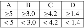
For a dataset containing four columns of features, considered as predictors, A, B, C, and D, and one column of class labels (E), 0 or 1, a decision tree can be constructed converting continuous data (Figure 2.6) into categorical data.

Figure 2.6: Information gain step one [6]

(42)

A B C D

≥5 ≥3.0 ≥4.2 ≥1.4

<5 <3.0 <4.2 <1.4

Table 2.1: Decision Tree Example: Feature Categorization

The information gain for each feature is found by first calculating the entropy of the target (in this case, it is a binary classification problem, the target is either 1 or 0, and there is 50/50 class balance, therefore the entropy of the target is 1), then calculating the entropy for each feature, and subtracting this entropy from the target entropy to yield the information gain. For example, the information gain for A is found as follows: 12 out of 16 records satisfy the cri-teria ≥5 (called criteria 1), and 4 out of 16 records satisfy the criteria <5 (called criteria 2). The number of positive class instances of criteria 1 is 5/12, and the number of negative class instances of criteria 2 is 7/12. Plugging this into equation 2.1 yields 0.9799. For criteria 2, the number of positive classes and negative classes is 3/4 and 1/4, respectively, yielding an entropy of 0.81128. The total entropy is then found by multiplying the number of instances A is≥5 by the entropy found in criteria 1, plus the number of instances A is<5 by the entropy found in criteria 2.

• For feature A≥5 and class==positive: ₁₂5

• For feature A≥5 and class==negative: ₁₂7

• Entropy(5,7)= −1[(₁₂5) log₂(₁₂5)+(₁₂7) log₂(₁₂7)]=0.9799

• For feature A<5 and class==positive: 3₄

• For feature A<5 and class==negative: 1₄

• Entropy(3,1)=-1[(3₄) log₂(3₄)+(1₄) log₂(1₄)]=0.81128

(43)

The information gain can then be found by subtracting the entropy of the target (1 because this is binary classification), by the entropy of feature A, yielding in this example 0.062255. Doing this for all four features (features), feature B is found to have the highest information gain of 0.707095, therefore by this method, it is known as the “best” feature and should be placed at the root node of the decision tree.

The gini index is used to measure how often a randomly chosen element would be incorrectly identified; therefore the feature with the lowest gini index is the best. The gini index is found for each criterion (as was done for the entropy detailed above), multiplied by the number of instances each criterion occurs within the dataset, and added to one another. Following the example above, for the same dataset with same criterion, the gini index for feature A can be found:

• For feature A≥5 and class==positive: ₁₂5

• For feature A≥5 and class==negative: ₁₂7

• gini(5,7)=1 - [(₁₂5)2+(₁₂7)2]=0.4860

• For feature A<5 and class==positive: 3₄

• For feature A<5 and class==negative: 1₄

• gini(3,1)=1-[(3₄)2+(1₄)2]=0.375

• gini(Target,A)=(12₁₆)×(0.486)+(₁₆4)×(0.375)=0.45825

Performing this on all four features, feature (feature) C yields the smallest gini index of 0.2, and therefore by this criteria would be chosen as the “best” feature to place at the node of the decision tree.

(44)

where the user splits the tree according to selected features, by first selecting the “best” feature for the root node, and secondly tree pruning, which consists of identifying and removing irrel-evant branches (such as those that lead to outliers) to increase the classification accuracy. Dis-advantages to the decision tree algorithm include a high probability of overfitting and a lower prediction accuracy as compared to other machine learning architectures, which is where the adaptation of this algorithm to a Random Forest becomes more useful in binary classification problems.

Random Forest

As mentioned, there are limitations to the decision tree model, which tends to have high vari-ance and is known for overfitting, leading to poor performvari-ance on the testing data. To combat for high variance and overfitting, the concept of Random Forest (RF) was introduced. A ran-dom forest is a type of classifier made up of many decision trees. The fundamental idea behind a random forest is to utilize an ensemble method of classification. It combines many decision trees into a single model and combines predictions made by these trees, thereby yielding im-proved predictive results when compared to a single decision tree. In the case of random forest, the model creates a “forest” of random, uncorrelated decision trees to arrive at the “best” pre-diction [67]. There are two particular instances of randomness in a random forest model, first in selecting the data observations to be used in the forest, and secondly in selecting a random set of features at each node to be evaluated.

Combining the trees, a random forest trains each tree on a slightly different set of data obser-vations, splitting the nodes in each tree on a limited number of features (chosen randomly). The final predictions of the random forest model are made by averaging the predictions of each tree. A random forest can be trained, for some number of trees, T, as follows:

(45)

that some samples will be used multiple times in a single tree, to create a subset of the data (for training, should be∼70-80% of the total dataset)

2. At each node:

(a) For some numberm,mfeatures are selected at random from all possible features

(b) The feature that provides the best split, according to the methodology chosen (i.e. gini or information gain), is used to do a binary split on that node

(c) At the following node, choose anothermfeatures and repeat

Figure 2.7 depicts an example of Random Forest architecture, with X representing the feature set representing the data of interest.

Figure 2.7: Random Forest Architecture [7]

Extremely Randomized Trees

(46)

1. splits nodes by choosing cut-points fully at random;

2. uses the whole learning sample to grow the trees (no boostrapping as in RF).

Choosing cut-points at random and using the entire learning sample to grow the trees introduces extra randomization as compared to the Random Forest model because instead of selecting an feature to split the node on based on the gini or information gain, the splitting feature is se-lected randomly. This methodology should be able to reduce variance more strongly than other, weaker randomization schemes. From a bias point of view, the usage of the full original learn-ing sample as opposed to bootstrap replicas can minimize model bias. From a computational point of view, the complexity of the tree growing procedure is on the order of NlogN, where

N is the learning sample size. Guerts, P. et. al. [8] describe the ERT algorithm well through pseudocode, shown in Figure 2.8 below:

(47)

Support Vector Machine

A Support Vector Machine (SVM) classifier aims to identify elements in each class by design-ing a hyperplane to divide the data into classes. Considerdesign-ing Figure 2.9, note that there are two classes of interest in this example (a case of binary classification), red squares and blue circles, and there are two features, x1, and x2. The green lines in Figure 2.9 show the possible

hyperplanes that could exist to separate each class accordingly.

Figure 2.9: Two-dimensional Support Vector Machine Example. [9].

The goal of the SVM classifier is to optimize the hyperplane such that the margin between the decision boundary (aka the hyperplane line shown in green) and the closest points from each class is maximized.

(48)

Figure 2.10: Two-dimensional Support Vector Machine Example. [9].

Figure 2.11: SVM Line to Plane [9].

Logistic Regression

(49)

known as features) and dependent variables (classes) [68]. The model that describes the re-lationship between the features and class expresses the predicted value of the class variable as the sum of products, where each product is formed by multiplying the feature value and the coefficient of the feature variable. The feature variable coefficient is obtained through a mathematical fit. The relationship between the feature and class variables is represented by an S-shaped Sigmoid curve. Using the Sigmoid curve, the LR function provides estimates be-tween 0 and 1. Logistic Regression is preferred over linear regression because of the Sigmoid curve describing the relationship between independent and dependent variables. For example, in linear regression, the line of best fit is denoted as:

y=mx+b (2.2)

Where y,x represent the x and y-coordinates of each point, m is the slope of the line, and b

the y-intercept. In logistic regression, the line of best fit is a Sigmoid curve represented by the equation:

y= 1

1+e−(mx+b) (2.3)

Figure 2.12 depicts the difference between linear and logistic regression, and visually shows why logistic regression is better suited for a binary classification problem (The data points at

y=0 represent the “0” class, and the data points aty= 1 represent the “1” class). The straight line (linear regression) attempts to fit all of the data to the line, which results in impossible predictions greater than one and less than zero.

The Sigmoid curve starts with a slow linear growth followed by exponential growth, ending again with a slow linear growth, and fits the data to the curve much better than the linear regression technique.

(50)

ap-Figure 2.12: Linear vs Logistic Regression [9].

plies a non-linear logarithmic transformation to the linear regression model [68]. LR requires each observation to be independent, and independent variables should not be linear functions of one another, but rather the independent variables should be linearly related to the logarith-mic probabilities of an event. Finally, LR requires large sample sizes because it uses maximum likelihood estimation.

2.5.4 Classification Performance Metrics

Confusion Matrix

(51)

Figure 2.13: Confusion Matrix [10]

Accuracy

Accuracy is the most common metric to test classifier performance, and is defined as the frac-tion of samples correctly predicted:

Accuracy= T P+T N

T P+T N+FP+FN (2.4)

Recall

The recall of a classifier is also known as it’s sensitivity, described as the fraction of positive events that were predicted correctly:

Recall= T P

T P+FN (2.5)

Precision

The precision of a classifier is the fraction of positive events identified by the classifier that are correctly identified as positive, described by:

Precision= T P

(52)

F1 score

The F1 score of a classifier is the harmonic mean of the recall and precision, described by:

F1= 2Precision∗Recall

Precision+Recall (2.7)

Classifiers aim for the highest F1 score possible which represents a better performing model.

Receiver Operating Characteristics Curve

The Receiver Operating Characteristics (ROC) curve is a probability curve which tells the capability of the classification model to distinguish between classes, with the True Positive Rate on the y-axis, and the False Postive Rate on the x-axis. The Area Under the ROC (AUC) curve is a percentage value between 0 and 1. The higher the AUC, the better the model is at predicting the 0 class as 0’s and the 1’s class as 1’s. Figure 2.14 depicts an example of an ROC curve. The dashed line represents an AUC = 0.5, an ROC curve for random guessing, and should be used as a baseline threshold for a model to perform above. With an AUC of 0.5, the model is not able to separate the classes, or has no class separation capacity, and performs no better than random guessing

Brier Score Loss

(53)

Figure 2.14: Confusion Matrix [11]

(54)

Classification of Accelerometer Data

At the time of this thesis completion, there has been no published literature using unprocessed satellite accelerometer data in machine learning for space weather applications. However, more and more work has been done in the fields of utilizing accelerometer and other motion sensor data to identify human activity and behaviour, and the techniques used in these works were utilized within this thesis. It has been shown by several authors (Leutheuser et. al. [70], Shoaib et. al. [71] and J.L. Reyes-Ortiz [72]) that machine learning classification techniques can be used for human activity recognition and provide accurate results.

3.1 Related Work

3.1.1 Classification of Human Activity with Accelerometer Data

Recent work done by Siirtola and R¨oning [72] used accelerometer data captured from users cellphones to delineate between five different human activities: idling, walking, cycling, run-ning, and driving. The authors used two types of classifiers, k-nearest-neighbours (knn) and quadratic discriminant analysis (QDA). They used a tri-axis accelerometer with a sampling

(55)

3.1. RelatedWork 37

frequency of 40Hz. A total of 21 features were extracted from the magnitude acceleration se-quences, standard deviation, mean, minimum, maximum, five different percentiles (10, 25, 50, 75, and 90), and a sum and square sum of observations above/below certain percentile (5, 10, 25, 75, 90, and 95). The same features were extracted from the signal where 2/3 acceleration channels were square summed together, generating a total of 42 features; 21 from the mag-nitude acceleration signal and 21 from the signal where the x and z component were square summed. The average recognition rate using QDA was 0.958, and the knn performed slightly worse with an average recognition rate of 0.939.

Most notably, the work done by E. Zdravevski et al. [12] heavily influenced the approach undertaken in this research, and will be detailed in the following subsections.

3.1.2 Benchmark Classification Model

(56)

Figure 3.1: Raw accelerometer readings for one hour during which two participants (a) male and (b) female, had a jogging activity [12]

3.1.3 Feature Selection

Feature selection was done manually, divided into six categories: basic statistics, equal-width histogram, percentile-based, correlations, auto-correlations, and curve fitting parameters. Fea-tures were extracted from twelve original time series with data segmented based on two strate-gies: 60 second windows without overlap, and 180 second with 120 second of overlap, in addition to time series derived from the original from both hip and ankle accelerometers. A flow diagram of the feature extraction, selection, and classification process is shown in 3.2.

3.1.4 Classifier Performance

(57)

3.1. RelatedWork 39

(58)

Figure 3.3: Classifier results 60 second windows [12]

(59)

Chapter 4 Methodology

The methodology of this thesis work from data acquisition to the final classifier model ar-chitecture can be described in the following overview, and will be detailed thoroughly in this chapter:

1. Data acquisition of the NASA JPL Level1B accelerometer data of the GRACE-A satel-lite;

2. First segmentation of daily data from 2002-2017 to dates with ICME storms as per the Richardson-Cane ICME list;

3. Pre-processing the raw data files to containing only the x-component of linear accelera-tion, time, and date (linear interpolation performed where necessary);

4. Class balancing to achieve a total dataset containing 50% ICME storms and 50% quiet days, 24-hour periods;

5. Feature extraction;

(a) Basic statistical features with percentiles extraction;

6. Random Forest methodology testing on 24-hour ICME periods, where at least 16/24

(60)

hours contain an ICME storm (regardless of Dst strength and Kp at the time of the storm);

7. Second segmentation of data, selecting 8-hour windows of ICME storms where at least 4/8 hours have a Dst index value less than -50, and 8-hour windows with Dst greater than -50 and Kp of 4 or less for the quiet periods;

8. RF, ERT, SVM, LR testing using basic statistical features with percentiles only with 10-fold cross validation (and testing on unseen data);

9. First-order derivative of data and extraction of basic statistical features;

10. Random Forest, ERT, SVM, LR testing using basic statistical features and first-order derivative features with 10-fold cross validation (and testing on unseen data);

11. Choosing RF and ERT architectures for further performance improvement;

12. Feature importance ranking and rejection of unimportant features of RF and ERT;

13. Hyperparameter tuning of RF and ERT using important features;

14. Selecting best hyperparameter settings to obtain final RF and ERT model and;

15. Testing RF and ERT final model on unseen test data (10% of data).

4.1 Data Acquisition

4.1.1 NASA JPL Level-1B Data

(61)

4.1. DataAcquisition 43

Level-0 data; sensor calibration factors are applied to convert the binary encoded measurements to engineering units. Time tag integer second ambiguity is resolved and data is time tagged with respect to the satellite receiver clock time, and editing and quality control flags are added. The Level-1A data can be reversible to Level-0, barring any bad data. The Level-1B data is then obtained through further processing, correctly time-tagging the data, and reducing the sample rate. Level-1B includes the ancillary data products generated during processing, and additional data needed for further processing. More information on the exact algorithms used for processing can be found in Sien-Chong Wu & Gerhard L.H. Kruizinga [73].

The accelerometer data used in this study is known as ACC1B, which provides the linear and angular acceleration components of the proof mass of the GRACE satellites. Due to the orientation of the spacecraft along its orbit path, only the x-component of linear acceleration is used in this study, as this is the acceleration component of the satellite that captures change due to space weather events. The SuperSTAR accelerometer used by GRACE-A has a highly-sensitive along-track (x) axis, which is the direction approximately tangential to its orbit path [18]. In the along-track direction, the main contribution to the non-conservation acceleration is caused by atmospheric drag, it therefore makes sense that the SuperSTAR accelerometer would capture changes in acceleration caused by an ICME event, since ICMEs cause perturbations to the atmosphere’s neutral density, thereby altering the drag force on GRACE-A. The drag acceleration is described by:

~a=−1

2ρv

2

rCD A M

~ vr

kv~rk

(4.1)

where ρis the atmospheric density, v~r the orbital velocity of the spacecraft, CD the drag

co-efficient,Athe equivalent cross-sectional surface perpendicular to the direction of motion and

(62)

Figures 4.1 and 4.2.

Figure 4.1: GRACE-A Acceleration during 8-hour Quiet Period November 2003

Figure 4.2: GRACE-A Acceleration during ICME Storm 8-hour Period November 2003

Visually, there is a clear difference between the accelerometer behaviour during an ICME storm, and during a period of quiet geomagnetic activity.

(63)

4.2. ClassBalancing 45

order to choose “quiet periods” that would account for seasonal changes of density in the atmosphere, every Wednesday from 2002-2017 (if ICME present on this day, then the next closest day was chosen) was selected as a reference quiet period (aka, a non-event as would be interpreted by the classifier). Therefore, 4 days per month, for every month from 2002-2017 over the lifetime of the GRACE-A mission (data availability permitting) was labelled as a “0” event. To confirm that there was no other geomagnetic activity on that day (in case it was missed by the Richardson-Cane list) the Dst index of that day was checked via [74]. Dst index is a good indication for geomagnetic activity caused by ICME storms. In addition, the Kp was also checked. “Quiet days” were rejected if their Dst index at any time during that day had a magnitude larger than 50, and their Kp index greater than 4+, if this occurred, the next closest day that was not during an ICME storm was chosen.

4.2 Class Balancing

(64)

4.2.1 Down-sampling and Window Selection Iteration One

The first iteration of down-sampling and class-balancing the data involved analyzing the storms and quiet periods over 24-hour windows. Each accelerometer file encompasses a 24-hour pe-riod, with one measurement taken every second with the exception of missing data that required interpolation. GRACE had an orbital period of∼94 minutes, therefore a 24-hour period would contain approximately ∼15 orbits of the satellite. Although the average storm length is ∼24 hours, to capture more of the storm data for the “1” class, storms between 16-24 hours were used. Storms shorter than 24 hours were “padded” with the data immediately before and/or after the occurrence of the event. It was initially hypothesised that two thirds of a 24-hour period and greater should be sufficient enough to extract a feature vector that would maintain the integrity of the satellite’s reaction to a storm event. In total, this method encompassed 69 ICME storms between 16-24 hours. For a 50/50 class balance, one quiet period for ev-ery ICME around the same time of year was taken. The newly-segmented, balanced dataset was first used in a Random Forest architecture to test its feasability prior to testing on all four classifier architectures, with details described in the Results section.

4.2.2 Down-sampling and Window Selection Iteration Two

(65)

Figure 4.3: GRACE-A Acceleration during 24-hour Quiet Period November 19th 2003

Figure 4.4: GRACE-A Acceleration during ICME Storm 24-hour period November 20th 2003

(66)

of September 19th-21st, 2005 shown in Figures 4.5 and 4.6.

Figure 4.5: GRACE-A Acceleration during 24-hour Quiet Period September 19th 2005

Figure 4.6: GRACE-A Acceleration during ICME Storm 24-hour period September 20th-21st 2005

(67)

the geo-effectiveness, or strength of the storm, is negligible from an atmospheric and satellite perturbation point of view. This is supported by the visual evidence of Figures 4.5 and 4.6 which show the GRACE-A satellite behaving similarly during a period of quiet activity and during a storm event. The September 2005 example, among many others over the lifetime of GRACE-A, was the motivation for the second down-sampling methodology described below.

(68)

Following the class-balancing, a 50/50 split of ICME storms and quiet days leave 174, 8-hour period samples to train and test a classifier with, 87 files per class. The limitations to the ma-chine learning model and space weather prediction capability using the described criteria is discussed in Chapter 6.

4.3 Pre-processing

4.3.1 Working with the raw files

(69)

4.3. Pre-processing 51

gaps of 10 seconds or shorter are filled using quadratic interpolation when at least 2 points per side are available. If there are less than two points per side, then linear interpolation is used to fill the data gap. Data gaps exceeding 10 seconds are not filled” [2]. Therefore, linear interpolation over the gaps was deemed to be sufficient in keeping the integrity of the dataset intact.

4.3.2 Extracting Feature Vectors

When extracting the feature vectors from the accelerometer data, [12]’s work was followed extensively. Their results show a classification accuracy of at least 0.99, using logistic re-gression, support vector machines, random forest, and extremely randomized trees machine learning algorithms. Data was first normalized using a max-min normalization method, and was calculated as follows: for every value V, there is a normalised value,VN that can be found

through:

VN =

V −minimum

maximum−minimum (4.2)

Basic Statistics with Percentiles

For Experiment one, a feature vector containing the 13 features was used. These features are based on basic statistics and percentiles, and include: minimum, standard deviation, mean, 25th percentile, 50th percentile, 75th percentile, maximum, range, median, geometric mean, variance, sum of series, and signal to noise ratio of the accelerometer data. The standard deviation of the data is described by:

σ= v t 1 N N X i=1

(70)

withN being the total sample size, xi representing the value of one sample,µthe mean of the

dataset, andσthe standard deviation.

The mean and geometric mean are calculated differently, with the mean shown in Equation 4.4 and the geometric mean in Equation 4.5:

µ= P

Xi

N (4.4)

where µ represents the mean, P

Xi is the summation of the samples, and N the number of

samples.

(ΠN_i₌₁xi) 1

N

(4.5)

The geometric mean is found by taking the Nth root of the multiplication of all samples (xi) in

a population, whereNrefers to the total number of samples.

The variance of a population is defined as the sum of the squared distances of each sample in the population from the meanµ, divided by the total number of samples N:

σ2 ₌

P

(X−µ)2

N (4.6)

The sum of series of a population is the sum of the time series values:

N−1

X

i=0

xi (4.7)

And the signal to noise ratio is defined as the mean of the samples divided by the standard deviation:

S NR= x¯

Machine Learning Classification of Interplanetary Coronal Mass Ejections Using Satellite Accelerometers

Scholarship@Western

Scholarship@Western

Machine Learning Classification of Interplanetary Coronal Mass

Machine Learning Classification of Interplanetary Coronal Mass

Ejections Using Satellite Accelerometers

Ejections Using Satellite Accelerometers

Lay Summary

Contents

List of Acronyms

Chapter 1

Introduction

1.1

Motivation

1.2

Tasks and Thesis Contribution

1.3

Thesis Outline

Chapter 2

Literature Review

2.1

Gravity Recovery and Climate Experiment

2.1.1

The STAR and SuperStar Accelerometers

2.2

Space Weather

2.2.1

Geomagnetic Storms

2.2.2

Interplanetary Coronal Mass Ejections

2.2.3

List of Richardson-Cane Interplanetary Coronal Mass Ejections

from 1996-2019

2.3

Earth’s Atmosphere

2.3.1

Atmospheric Response to Solar Events

2.3.2

Satellite Response to Solar Events

2.4

Space Weather Monitoring

2.4.1

Previous Work

2.4.2

Instrumentation for Interplanetary Coronal Mass Ejection

Identi-fication

2.4.3

The Use of Satellite Accelerometers for Space Weather Monitoring

2.4.4

Space Weather Monitoring with Machine Learning

2.5

Machine Learning for Classification

2.5.1

Features and Feature Sets

2.5.2

Training, Testing, and Validation Sets

2.5.3

Supervised Learning

2.5.4

Classification Performance Metrics

Classification of Accelerometer Data

3.1

Related Work

3.1.1

Classification of Human Activity with Accelerometer Data

3.1.2

Benchmark Classification Model

3.1.3

Feature Selection

3.1.4

Classifier Performance

Chapter 4

Methodology

4.1

Data Acquisition

4.1.1

NASA JPL Level-1B Data

4.2

Class Balancing

4.2.1