Approximate Integer Common Divisor Problem relates
to Implicit Factorization
Santanu Sarkar and Subhamoy Maitra
Applied Statistics Unit, Indian Statistical Institute, 203 B T Road, Kolkata 700 108, India
{santanu r, subho}@isical.ac.in
Abstract. In this paper, we analyse how to calculate the GCD of k (≥ 2) many large integers, given their approximations. Two versions of the approximate common divisor problem, presented by Howgrave-Graham in CaLC 2001, are special cases of our analysis when k = 2. We then relate the approximate common divisor problem to the implicit factorization problem. This has been introduced by May and Ritzenhofen in PKC 2009 and studied under the assumption that some of Least Significant Bits (LSBs) of certain primes are same. Our strategy can be applied to the implicit factorization problem in a general framework considering the equality of (i) Most Significant Bits (MSBs), (ii) Least Significant Bits (LSBs) and (iii) MSBs and LSBs together. We present new and improved theoretical as well as experimental results in comparison with the state of the art works in this area.
Keywords:Greatest Common Divisor, Factorization, Integer Approximations, Implicit Fac-torization, Lattice, LLL.
1
Introduction
It is known that given two large integers a, b (a > b), one can calculate the GCD efficiently in O(log2a) time [STN02, Page 169]. In [HOW01], Howgrave-Graham has shown that it is possible to calculate the GCD efficiently when some approximations ofa, bare available. This problem was referred as “approximate common divisors”. Using the strategy of [HOW01], Coron and May [COR07] proved the deterministic polynomial time equivalence of computing the RSA secret key and factoring.
In a recent paper [MAY09], May and Ritzenhofen explained the problem of implicit factorization. The motivation of this problem in the context of oracle complexity has nicely been explained in [MAY09]. Thus we directly get into the problem description. Consider
N1 = p1q1, N2 = p2q2, . . . , Nk = pkqk, where p1, p2, . . . , pk and q1, q2, . . . , qk are primes. It
is also considered that p1, p2, . . . , pk are of same bit size and so are q1, q2, . . . , qk; this is
followed throughout the paper unless otherwise mentioned. Given that certain portions of bit pattern inp1, p2, . . . , pk are common, the question is under what conditions it is possible
to factor N1, N2, . . . , Nk efficiently. In [MAY09], the result was based under the assumption
that some amount of LSBs are same in p1, p2, . . . , pk. Later, in [SAR09], different cases has
of [SAR09] has been improved. Note that the work of [FAU10] and certain part of this work (Sections 2, 3, except Section 3.1) [SAR10] are done independently at the similar time.
In this paper we concentrate on the implicit factorization problem considering some amount of (i) MSBs or (ii) LSBs or (iii) MSBs as well as LSBs are same in p1, p2, . . . , pk.
Thus the work of [MAY09] (the LSB case) as well as that of [FAU10] (the work for MSB case) are considered in the same framework. Further, the technique takes care of the case considering some portions of MSBs and LSBs together. Our work is of the same quality (in general) and slightly improved (in certain cases) in comparison to [MAY09,FAU10]. We generalize the ideas of [HOW01] for the lattice based technique that we exploit in this paper and our strategy is different from that of [MAY09,SAR09,FAU10].
First consider k = 2. Asp1, p2 share certain amount of MSBs, one can writep1−p2 =x0, where x0 is of lesser bit size than p1 orp2. Hence N2 = (p1−x0)q2. Therefore, gcd(N1, N2+
x0q2) =p1. Since, N2 (known) is an approximation of N2+x0q2 (unknown), we can use the technique of [HOW01] to solve this problem efficiently and get p1 under certain conditions. This gives factorization of N1. Additionally, when p1 > x0q2, then either bNp12c or dNp12e will provide q2. This is explained in detail in Section 2.1.
Next we generalize the PACDP given in [HOW01]. Let a1, a2, . . . , ak are integers with
gcd(a1, a2, . . . , ak) =g. Supposea(0)2 , . . . , a (0)
k are given which are approximations ofa2, . . . , ak
respectively. We like to find g from the knowledge of a1, a(0)2 , . . . , a (0)
k . An immediate
appli-cation of our general version towards the implicit factorization is as follows. We can write
p1 =p1+x1, . . . , pk =p1+xk where x1 = 0. Hence p1 = gcd(N1, N2−x2q2, . . . , Nk−xkqk)
and consequently, we can find x2q2, . . . , xkqk under certain conditions.
For application of the results related to approximate integer common divisor to implicit factorization, we need to generalize the PACDP [HOW01]. Let us describe the problem which we name as Extended Partially Approximate Common Divisor Problem (EPACDP).
Definition 1. EPACDP.
Let a1, a2, . . . , ak be large integers of same bit size and g =gcd(a1, a2, . . . , ak). Consider that
a(0)2 , . . . , a(0)k are the approximations of a2, . . . , ak respectively and a(0)2 , . . . , a (0)
k are of same
bit size too. Let a2 =a(0)2 +x (0)
2 , . . . , ak =a
(0)
k +x
(0)
k . We need to find x
(0) 2 , . . . , x
(0)
k from the
knowledge of a1, a(0)2 , . . . , a (0)
k .
The PACDP of [HOW01] considers only a1, a2. For application to implicit factorization, we get one of the integers, denoted by a1 in Definition 1, exactly and the rest of the integers
a2, . . . , ak as approximations.
The problem when a1 is not available exactly, but an approximation of a1 is available, is referred as General Approximate Common Divisor Problem (GACDP) in [HOW01]. One can extend it as follows with the name Extended General Approximate Common Divisor Problem (EGACDP). The GACDP of [HOW01] considers only a1, a2.
Definition 2. EGACDP.
Let a1, a2, . . . , ak be large integers of same bit size and g =gcd(a1, a2, . . . , ak). Consider that
are of same bit size too. Let a1 =a(0)1 +x (0)
1 , a2 =a(0)2 +x (0)
2 , . . . , ak=a
(0)
k +x
(0)
k . We need to
find x(0)1 , x(0)2 , . . . , x(0)k from the knowledge of a(0)1 , a(0)2 , . . . , a(0)k .
Since for the implicit factorization problem we geta1 exactly, EPACDP maps directly to it.
Contribution and Roadmap:
– We generalize the partially approximate common divisor problem (PACDP) [HOW01] in Section 2 and show how our generalized version applies to the implicit factorization problem described in [MAY09].
– In Section 2.1, we apply our result for the case k = 2 and show when we can achieve better theoretical result than that of [SAR09]. The implicit factorization problem while the MSBs are equal could be handled in [SAR09] only fork = 2. We also explain the case for k = 3 in Section 2.2 to detail our technique.
– The results of Section 2 are approximated in a closed form expression using a sublattice structure in Section 3. For simplicity we initiate our discussion with the case (i) when the primes p1, . . . , pk share some amount of MSBs. However, a little modification of
our strategy (presented in Section 3.1) shows that the method works as well for the cases (ii) when the primes p1, . . . , pk share some amount of LSBs and also (iii) when the
primes p1, . . . , pk share some amount of MSBs as well as LSBs. Based on this we present
closed form bounds for the solution for implicit factorization when p1, . . . , pk share some
amount of bits. To show the improvements, our results are compared in detail with that of [MAY09,SAR09,FAU10].
– We also exploit another recently presented technique [DJK09] for calculation of approxi-mate common divisor. Though the theoretical bound of this technique is worse than that of our results in Section 3, we can utilize it for better experimental performance. This is presented in Section 4.
– Moreover, we study the EGACDP, the generalization of GACDP [HOW01] in Section 5.
2
The General Solution for EPACDP
Towards solving the EPACDP, consider the polynomials
h2(x2, . . . , xk) = a(0)2 +x2,
. . . ,
hk(x2, . . . , xk) = a(0)k +xk, (1)
where x2, . . . , xk are the variables. Clearly g (as in Definition 1) divides hi(x(0)2 , . . . , x(0)k ) for
2≤i≤k.
Now let us define the shift polynomials
h0,...,0,j2,...,jk(x2, . . . , xk) =h
j2
2 . . . h
jk
ka
m−j2−...−jk
for non-negative integers ji, 2≤i≤k such that j2+. . .+jk ≤m where the integer m ≥0
is fixed.
Further, we define another set of shift polynomials
h0,...,0,in,0,...,0,j2,...,jk(x2, . . . , xk) = x
in
nh j2
2 . . . h
jk
k , (3)
with the following: (i) 1≤in ≤t, for 2≤n ≤kand a positive integert, and (ii)j2+. . .+jk=
m, when 0 ≤j2, . . . , jn−1 < in, and 0≤jn, . . . , jk ≤m.
We also need the following heuristic assumption to proceed.
Assumption 1.Consider a set of polynomials {f2, f3, . . . , fk}onk−1 variables having the
root of the form (x(0)2 , . . . , x(0)k ). Then we will be able to collect the root efficiently using resultants.
Let us now state the following result due to Howgrave-Graham [HOW97].
Lemma 1. Let h(x2, . . . , xk) ∈ Z[x] be the sum of at most ω monomials. Suppose that
h(x(0)2 , . . . , x(0)k )≡0 modNm where |x(0)2 | ≤X2, . . . ,|x(0)k | ≤Xk and ||h(x2X2, . . . , xkXk)||< Nm
√
ω. Then h(x
(0) 2 , . . . , x
(0)
k ) = 0.
We also note that the basis vectors of an LLL-reduced basis fulfill the following prop-erty [LLL82,MAY03] (see also [ELN07, Theorem 3.2, Page 22]).
Lemma 2. Let L be an integer lattice of dimension ω. The LLL algorithm applied on L outputs a reduced basis of L spanned by {v1, . . . , vω} with
||v1|| ≤ ||v2|| ≤. . .≤ ||vi|| ≤2
ω(ω−1)
4(ω+1−i) det(L)ω+11−i, for i= 1, . . . , ω,
in polynomial time of dimension ω and the bit size of the entries of L.
Note thatgm divides any shift polynomialh
...(x(0)2 , . . . , x (0)
k ). LetX2, . . . , Xk be the upper
bounds ofx(0)2 , . . . , x(0)k respectively. Now we define a latticeLusing the coefficient vectors of
h...(x2X2, . . . , xkXk). Let the dimension ofLbeω. Under Assumption 1, one getsx(0)2 , . . . , x (0)
k
using lattice reduction overL, if 24(ωω(+2ω−−1)k) det(L)ω+21−k < g m
√
ω. The result follows from Lemma 1
and putting i=k−1 in Lemma 2. Neglecting the small constants and considering k << ω
(in fact, we will show that ω is exponential in k in our construction), we get the condition as det(L)ω1 < gm, i.e., det(L)< gmω. This is written formally in Theorem 1 later.
Before proceeding to the next discussion, we denote that n r
is considered in its usual meaning when n ≥r ≥0 and in all other cases we will consider the value of nr
as 0.
Lemma 3.
ω=
m
X
r=0
k+r−2
r
+
k
X
n=2
t
X
in=1
n−2
X
r=0 (−1)r
n−2
r
k+m−rin−2
m−rin
Proof. Let j2 +. . .+jk = r where ji ≥ 0 for 2 ≤ i ≤ k. The number of such solutions is k+r−2
r
. Hence the number of shift polynomials in Equation 2 isω1 =
m
X
r=0
k+r−2
r
.
For fixedn, in, the number of shift polynomials in Equation 3 is the number of all possible
solutions of j2 +. . .+jk = m for 0 ≤ j2, . . . , jn−1 < in, and 0 ≤ jn, . . . , jk ≤ m. Now
the number of all possible solutions of j2 +. . .+jk = m for 0 ≤ j2, . . . , jn−1 < in, and
0 ≤ jn, . . . , jk ≤ m is the co-efficient of xm in (1 + x +. . . + xin−1)n−2(1 + x + . . .+
xm)k−n+1 and we denote the coefficient byc(n, i
n), as we have fixedn, in. Now (1 +x+. . .+
xin−1)n−2(1+x+. . .+xm)k−n+1= (1−xin
1−x )
n−2(1−xm+1
1−x )
k−n+1 = (1−xin)n−2(1−xm+1)k−n+1(1−
x)−k+1. Hence c(n, i
n) will be the co-efficient of xm in (1 −xin)n−2(1− x)−k+1. We have
(1−xin)n−2 =
n−2
X
r=0 (−1)r
n−2
r
xinr and (1
−x)−k+1 = ∞ X
r=0
k+r−2
r
xr. So, c(n, in) =
n−2
X
r=0 (−1)r
n−2
r
k+m−rin−2
m−rin
. Hence the number of shift polynomials in Equation 3
is ω2 =
k
X
n=2
t
X
in=1
c(n, in). Finally,ω =ω1 +ω2 provides the result. ut
Lemma 4. The determinant of L is given by det(L) =P1P2 where
P1 =
Y
Xj2
2 X
j3
3 . . . X
jk
k a
m−j2−...−jk
1
for non-negative integers ji, 2≤i≤k such that j2 +. . .+jk ≤m, and
P2 =
Y
Xin
n X j2
2 X
j3
3 . . . X
jk
k with the following: (i) 1 ≤ in ≤ t, for 2 ≤ n ≤ k and
a positive integer t, and (ii) j2 + j3 +. . . +jk = m, when 0 ≤ j2, . . . , jn−1 < in, and
0≤jn, . . . , jk ≤m.
Proof. The matrix (corresponding to the latticeL) containing the basis vectors is triangular and has the following two kinds of diagonal entries:
Xj2
2 X
j3
3 . . . X
jk
k a
m−j2−...−jk
1 , (4)
for non-negative integers ji, 2≤i≤k such that j2+. . .+jk ≤m where the integer m ≥0
fixed and
Xin
n X j2
2 X
j3
3 . . . X
jk
k , (5)
with the following: (i) 1≤ in ≤ t, for 2≤ n ≤k and a positive integer t, and (ii) j2 +j3+
. . .+jk=m, when 0≤j2, . . . , jn−1 < in, and 0≤jn, . . . , jk ≤m.
Clearly P1 is the product of the elements from (4) and P2 is the product of the elements
from (5). Hence det(L) =P1P2. ut
lattice dimension in our case is exponential in k so the running time of our strategy is poly{loga1,exp(k)}. Thus, for small fixed k our algorithm is polynomial in loga1. Now, we have the following main result.
Theorem 1. Under Assumption 1, the EPACDP (as in Definition 1) can be solved in poly{loga1,exp(k)} time when det(L) < gmω, where det(L) is as in Lemma 4 and ω is
as in Lemma 3.
One may also consider the same upper bound on the errorsx(0)2 , . . . , x(0)k . In that case we get the following result.
Corollary 1. Considering the same upper bound X on the errors x(0)2 , . . . , x(0)k , we have
det(L) =P1P2 where
P1=X
Pm
r=0r(
k+r−2
r )a
Pm
r=0(m−r)(
k+r−2
r )
1 ,
P2=X
k
X
n=2
t
X
in=1
(in+m) n−2
X
r=0 (−1)r
n−2
r
k+m−rin−2
m−rin
.
Proof. LetX2 =X3 =. . .=Xk=X. Then from (4), we have
Xj2
2 X
j3
3 . . . X
jk
k a
m−j2−...−jk
1 =Xj2+...+jka
m−j2−...−jk
1 , for non-negative integers ji, 2≤i≤k
such that j2 +. . .+jk ≤ m. Let j2+. . .+jk = r where 0 ≤ r ≤ m. The total number of
such representation is k+r−2
r
. Hence
P1 =
m
Y
r=0
(Xram−r
1 )(
k+r−2
r ) = X
Pm
r=0r(
k+r−2
r )a
Pm
r=0(m−r)(
k+r−2
r )
1 .
For calculating P2, we have the following constraints: (i) 1 ≤ in ≤ t, for 2 ≤ n ≤ k and
a positive integer t, and (ii) j2 +j3 + . . .+ jk = m, when 0 ≤ j2, . . . , jn−1 < in, and
0≤jn, . . . , jk ≤m. Thus,
P2=
k
Y
n=2
t
Y
in=1
Xin
n X j2
2 X
j3
3 . . . X
jk k = k Y n=2 t Y
in=1
Xinc(n,in)Xmc(n,in)
=XPkn=2
Pt
in=1(in+m)Prn=0−2(−1)r(
n−2
r )(
k+m−rin−2
m−rin ).
u t
As the results in this section are quite involved, we present below a few cases for better understanding and comparison with existing results.
2.1 Analysis for k = 2
common divisor problem (PACDP) [HOW01] has been exploited. As described in [COP97], after applying LLL, if the output polynomials are of more than one variable, then to collect the roots from these polynomials one needs, Assumption 1. However, in this case, Assumption 1 is not required since there is only one variable in the polynomial that we will consider.
Theorem 2. Let N1 = p1q1 and N2 = p2q2, where p1, p2, q1, q2 are primes. Let N ≈ N1 ≈
N2, q1, q2 ≈ Nα and |p
1 −p2| < Nβ. Then one can factor N1 and N2 deterministically in
poly(logN) time when β <1−3α+α2, provided2α+β ≤1.
Proof. Let x0 = p1 −p2. We have N1 = p1q1 and N2 = p2q2 = (p1 −x0)q2. Our goal is to recover x0q2 from N1 and N2. Since |x0| < Nβ and q2 =Nα, we can take X = Nα+β as an upper bound ofx0q2. Now we consider the shift polynomials
gij(x) = xi(N2 +x)jN1m−j (6)
fori= 0, 0≤j ≤ m and j =m, 1≤i≤t,
where m, tare fixed non-negative integers. Clearly, gij(x0q2)≡0 mod (pm1 ).
We construct the lattice Lspanned by the coefficient vectors of the polynomials gij(xX)
in (6). One can check that the dimension of the latticeLisω=m+t+1 and the determinant of L is
det(L) =X(m+t)(m2+t+1)N
m(m+1) 2
1 ≈X
(m+t)(m+t+1)
2 N
m(m+1)
2 . (7)
Here, P1 = X
m(m+1)
2 N
m(m+1)
2 and P2 = Xmt+
t(t+1)
2 (the general expressions of P1, P2 are presented in Lemma 4). Using Lattice reduction on L by LLL algorithm [LLL82], one can find a non-zero vector b whose norm ||b|| satisfies ||b|| ≤ 2ω−41(det(L))
1
ω. The vector b is
the coefficient vector of the polynomial h(xX) with ||h(xX)|| = ||b||, where h(x) is the integer linear combination of the polynomials gij(x). Hence h(x0q2)≡0 mod (pm1 ). To apply Lemma 1 and Lemma 2 for finding the integer root of h(x), we need
2ω−41(det(L)) 1
ω < p
m
1
√
ω. (8)
Neglecting small constant terms, we can rewrite (8) as det(L) < pmω
1 . Substituting the expression of det(L) from (7) and using X =Nα+β, p
1 ≈N1−α we get (m+t)(m+t+ 1)
2 (α+β)< m((1−α)(m+t+ 1)−
m+ 1
2 ). (9)
Lett =τ m. Then neglecting the terms of o(m2) we can rewrite (9) as
ψ(α, β, τ) = (−α−β)τ 2
2 + (−2α−β+ 1)τ+ (− 3α
2 −
β
2 + 1
2)>0. (10)
The optimal value of τ, to maximize β for a fixed α isτ = 1−β−2α
α+β . Since τ ≥0 we need
Putting the optimal value ofτ in (10), we get
α2−3α−β+ 1>0. (12)
Oncex0q2, the integer root ofh(x), is known, we getp1 by calculating the GCD of N1, N2+
x0q2. As long as |x0q2|< p1, we get q2 by calculating the floor or ceiling of N2
p1. As |x0q2| ≤
Nα+β and p
1 ≈N1−α, to satisfy |x0q2| ≤ p1 we need 2α+β ≤ 1 which is incidentally same as (11).
Our strategy uses LLL [LLL82] algorithm to findh(x) and then calculates the integer root of h(x). Both these steps are deterministic polynomial time in logN. Thus the result. ut
The relation presented in (9) provides the bound when the lattice parameters m, tare spec-ified. The asymptotic relation independent of the lattice parameters has been presented in (12). This is the theoretical bound and may not be reached in practice as we work with low lattice dimensions. Now let us compare our results with that of [SAR09].
0.1 0.15 0.2 0.25 0.3 0.35 0.4 0.45 0.5
0 0.2 0.4 0.6 0.8
α→
Upper bound of
β
→
case(i) case(ii) case(iii)
Fig. 1.Comparison of our theoretical result [case (i), works for both MSBs and LSBs] with that of [MAY09] [case (ii), works for LSBs], [FAU10] [case (ii), works for MSBs] and [SAR09] [case (iii), works for MSBs].
1. In [SAR09, Theorem 2.1] it has been explained that factorization will be successful when
Ψ(α, β) = 4α2+ 2αβ +14β2 −4α− 53β+ 1 > 0 provided 1− 32β−2α ≥ 0. In our case, the upper bound of β is α2−3α+ 1. Putting this upper bound of β in Ψ we get Ψ <0 whenα ≤0.33. Hence upper bound ofβ in our case will be greater than of [SAR09] when
α ≤0.33.
3. The result of [SAR09] could not be extended for k > 2, but our result can be extended for general k.
4. We get similar quality of experimental results as in [SAR09] and both the experimental results (i.e., our and that of [SAR09]) almost coincide with our theoretical results. Our experimental results are same as our theoretical results following (9) for specific lattice dimensions, whereas the experimental results of [SAR09] are better than the theoretical results of [SAR09] as explained in [SAR09, Remark 2].
We also like to compare our result with that of [MAY09,FAU10]. The strategy of [MAY09] considers equality in some LSBs of p1, p2. One may note that our theoretical results for the MSB case is same as that of the LSB case (see Section 3.1 later). The strategy of [MAY09] works when β ≤ 1−3α. In our case, β < 1−3α+α2. It is thus immediate to see that our upper bound is better than that of [MAY09]. Given α, the amount of bit sharing is (1−α− β) log2N. Thus, for k = 2, we need smaller number of bit sharing in LSBs for implicit factorization than the number of bit sharing in LSBs achieved in [MAY09]. For
k = 2, the strategy of [FAU10] works in the MSB case when β ≤ 1−3α− log3
2N, and thus it is clear that our theoretical result is better than [FAU10] for the MSB case. Later in Section 3, we will compare our results with that of [MAY09,FAU10] for all k ≥2.
One may refer to Figure 1 for the comparison of the theoretical results. The curve for the theoretical result given in [FAU10] (MSB case) will be parallel and slightly below that of the curve for [MAY09] (LSB case) and that is why we have not drawn it separately.
2.2 Analysis for k = 3
As we have already pointed out, the idea of [SAR09] could not be extended for k > 2. However, our technique works in the general case. We now explain the case for k = 3 in detail.
Theorem 3. Let N1 = p1q1, N2 = p2q2 and N3 = p3q3, where p1, p2, p3, and q1, q2, q3 are
primes. LetN, N1, N2, N3 be of same bit size andq1, q2, q3 ≈Nα, |p1−p2|< Nβ, |p1−p3|<
Nβ. Then, under Assumption 1, one can factor N
1, N2 and N3 in poly(logN) time when
β <(1−α)32 −α, provided 2α+β ≤1.
Proof. Letx0 =p2−p1 andy0 =p3−p1. We have N1 =p1q1, N2 =p2q2 = (x0+p1)q2, N3 = (y0 +p1)q3. Our goal is to recover x0q2, y0q3 from N1, N2 and N3. Let X = Nα+β. Clearly
X is an upper bound of x0q2, y0q3. Also we have p1 ≈ N1−α. When k = 3 then P1 =
Xm
3
3 +o(m3)N
m3
6 +o(m3).
Let t =τ m. To have a manageable formula for P2, we need to assume t≤ m+ 1. Then
P2 =Xm
3τ2+m3τ+m3τ3
3 +o(m3) and ω = m 2
2 +m
2τ+m2τ2
2 +o(m 2).
Neglecting the o(m3) terms, the required condition det(L) < pmω
1 implies (13 +τ
2+τ +
τ3
3 )(α+β) + 1
6 <(1−α)( 1
2 +τ +
τ2
2), i.e.,
−1
3τ 3α
− 1
3τ 3β
− 3
2τ 2α
−τ2β+ 1 2τ
2
−2τ α−τ β +τ − 5
6α− 1 3β+
1
To maximize β for a fixed α, the optimal value of τ is 1−2α−β
α+β . Putting this optimal value
of τ in (13), we get the required condition as −α3 + 2α2 −2αβ − β2 −3α + 1 > 0, i.e.,
β <√1−3α+ 3α2−α3−α. As τ ≥0, we also need the constraint 2α+β ≤1. Then under Assumption 1 (as the polynomials are of two variables), we can collect the roots successfully.
u t
3
Sublattice and Generalized Bound
In this section, we study a sublattice L0 of the lattice L explained in the previous section. This helps in two ways as follows.
– The dimension of the sublattice L0 is less than that of L and this helps in actual experi-ments.
– The theoretical analysis helps us to get a generalized bound for β.
We need the following technical result that will be used later.
Lemma 5. For any fixed positive integer r ≥ 1, and a large integer m,
m
X
t=1
tr = m
r+1
r+ 1 +
o(mr+1).
Proof. Let S = 1r+ 2r+. . .+mr. Then, Rm
0 x
rdx < S < Rm+1
1 x
rdx. Thus, mr+1
r+1 < S < (m+1)r+1−1
r+1 , which gives,
mr+1
r+1 < S <
(m+1)r+1
r+1 . Now,
(m+1)r+1
r+1 −
mr+1
r+1 contains the terms m
i
for i≤r. Thus, for a fixed r and large m, one can write S = mr+1
r+1 +o(m
r+1). ut
Now we present the main result describing the bound on β.
Theorem 4. Consider EPACDP with g ≈ a1−α
1 and x (0)
2 ≈ . . .≈x (0)
k ≈a α+β
1 . Then, under
Assumption 1, one can solve EPACDP in poly{loga,exp(k)} time when
β < k
2+ 5αk−2αk2−2α−2k+ 1−√k2+ 2α2k−α2k2−2k+ 1
k2−3k+ 2 for k > 2 and
<1−3α+α2, for k = 2,
with the constraint 2α+β≤1.
Proof. We start by explaining the shift polynomials. First we consider the following ones which are same as given in (2) in the previous section.
h0,...,0,j2,...,jk(x2, . . . , xk) =h
j2
2 . . . h
jk
ka
m−j2−...−jk
1 , (14)
for non-negative integers ji, 2≤i≤k such that j2+. . .+jk ≤m where the integer m ≥0
fixed.
Further, we define another set of shift polynomials which is a sub-collection of the poly-nomials presented in the last section in (3),
hi2,0,...,0,0,...,0,j2,...,jk(x2, . . . , xk) = x
i2
2h
j2
2 . . . h
jk
with the following: (i) 1≤i2 ≤t, for a positive integert, and (ii)j2+. . .+jk=m, andji ≥0
for 2≤i≤k. Next we define a latticeL0 using the coefficient vectors ofh
...(x2X2, . . . , xkXk).
LetX2 =X3 =. . .=Xk =X, the common upper bound. The shift polynomials from (14)
contribute P0 1 =
m
Y
r=0
(Xram−r
1 )(
k+r−2
r ) =X
Pm
r=0r(
k+r−2
r )a
Pm
r=0(m−r)(
k+r−2
r )
1 to the determinant of
L0. (This P0
1 is same as P1 in Corollary 1.) The shift polynomials from (15) contribute P20 =
t
Y
i2=1
(Xi2Xm)(k+mm−2) =X
t
X
i2=1
(i2+m)
k+m−2
m
to the determinant of L0. The dimension
of L0 is ω0 =
m
X
r=0
k+r−2
r
+t
m+k−2
m
.
Now, k+r−2
r
= (r+1)...(r+k−2) (k−2)! =
rk−2
(k−2)! +o(r
k−2). Then,
P1 ≈ X
Pm
r=0rrk −2 (k−2)!a
Pm
r=0(m−r)
rk−2 (k−2)!
1 ≈ X
1 (k−2)!
mk k a
1 (k−2)!
mk k−1−
1 (k−2)!
mk k
1 , using Lemma 5 and
neglecting the lower order terms. Moreover,
P2 = X
Pt
i2=1(i2+m) mk−2
(k−2)! ≈ X(k−12)!(
t2mk−2
2 +tmk−1), (neglecting the lower order terms). Fur-ther,
ω0 ≈ Pm
r=0
rk−2
(k−2)! + t
mk−2
(k−2)! ≈
mk−1
(k−1)(k−2)! + t
mk−2
(k−2)!, (using Lemma 5 and neglecting the lower order terms). Following Lemma 1, the required condition is det(L0) = P0
1P20 < gmω 0
, where g is the common divisor. Let g =a1−α
1 , X =a
α+β
1 . Then putting the values of g, X in det(L0) =P0
1P20 < gmω 0
, we get,
(m
k
k +
mk−2t2
2 +m
k−1t)(α+β) + mk
k−1 −
mk
k <(1−α)(m
k−1t+ mk
k−1). (16)
Now putting t=τ m, (τ ≥0 is a real number) in (16), we get the condition as
(1
k +
τ2
2 +τ)(α+β) + 1
(k−1)k <(1−α)(τ+
1
k−1). (17)
To maximizeβ for a fixedα, the optimal value ofτ isτ = 1−2α−β
α+β . Putting this optimal value
in (17), we get the condition as 4α2k2+ 4αβk2+β2k2−8α2k−10αβk−3β2k−4αk2−2βk2+ 2α2+4αβ+2β2+6αk+4βk+k2−2α−2β−k >0. From which we get the required condition asβ < k2+5αk−2αk2−2α−2k+1−√k2+2α2k−α2k2−2k+1
k2−3k+2 whenk > 2 andβ <1−3α+α2 whenk = 2.
Since τ ≥0, we also need the constraint 1−2α−β ≥0. Then under Assumption 1 (as the polynomials are of more than one variable), we can collect the roots successfully. ut
3.1 Implicit Factorization problem with shared MSBs and LSBs together
takes care of the case when only LSBs are shared. As before, consider N1 = p1q1, N2 =
p2q2, . . . , Nk = pkqk, where p1, p2, . . . , pk and q1, q2, . . . , qk are primes. It is also considered
that p1, p2, . . . , pk are of same bit size and so are q1, q2, . . . , qk. We also assume that some
amount of LSBs as well as some amount of MSBs of p1, p2, . . . , pk are same.
Theorem 5. Let q1, q2, . . . , qk ≈ Nα. Consider that γ1log2N many MSBs and γ2log2N
many LSBs of p1, p2, . . . , pk are same. Let β = 1−α−γ1−γ2. Then, under Assumption 1,
one can factor N1, N2, . . . , Nk in poly{loga,exp(k)} if
β < k
2+ 5αk−2αk2−2α−2k+ 1−√k2+ 2α2k−α2k2−2k+ 1
k2−3k+ 2 for k > 2 and
<1−3α+α2, for k = 2.
with the constraint 2α+β≤1.
Proof. It is given that γ1log2N many MSBs and γ2log2N many LSBs of p1, p2, . . . , pk are
same. Thus, we can write
p2=p(0)1 +N
γ2x(0)
2 ,
p3=p(0)1 +Nγ2x (0) 3 ,
. . .
pk=p(0)1 +Nγ2x (0)
k .
Using the above relations, we have,
Niq1−N1qi =Nγ2x(0)i qiq1 for 1< i ≤k. (18)
Suppose, aNγ2 ≡ 1 modN
1. Now multiplying Equation 18 by a, we get aNiq1 −x(0)i qiq1 ≡ 0 modN1.
Let bi ≡ aNi modN1 for 1 < i ≤ k. Thus we have, biq1 −x(0)i qiq1 ≡ 0 mod N1. From which, we get bi−x(0)i qi ≡0 modp1 for 1< i≤k. Hence our first aim is to findx(0)i qi from
N1 and bi for 1< i≤k. Then from the knowledge of x(0)i qi, we want to find the factorization
of Ni for 1 ≤ i ≤ k. Here we have x(0)i ≈ N1−α−γ1−γ2 for 1 ≤ i ≤ k. Then following the
similar technique as in the proof of Theorem 4, the desired result is achieved. ut
We extend the results related to MSBs (as in Theorem 4 and earlier) in case of LSBs or MSBs and LSBs taken together (as in Theorem 3.1). This is achieved by exploiting the idea of a where, aNγ2 ≡1 mod N
1 and then multiplying the equations by a.
This is the first time a solution could be achieved considering sharing of MSBs and LSBs together for general k. This has been studied fork = 2 in [SAR09] and it has been left as an open problem in [FAU10].
3.2 Comparison with the work of [MAY09,FAU10]
Let us now compare our result with that of [MAY09] for the general case. The strategy of [MAY09] considers equality in some LSBs of p1, p2, . . . , pk and we consider the same here
following the result in Section 3.1.
The strategy of [MAY09] works when β≤1−α−kk
−1α= 1− 2k−1
k−1α. As β >0, one may note α < k−1
2k−1, i.e, α < 1 2.
We have already discussed in Section 2.1 that for the casek = 2 our result is better than that of [MAY09]. The results of Theorem 4 for k = 2 and Theorem 2 are same, sinceL and
L0 are same for k = 2. However, L and L0 become different fork > 2. For k > 2, k2+5αk−2αk2−2α−2k+1−√k2+2α2k−α2k2−2k+1
k2−3k+2 >1− 2
k−1
k−1α. Thus, for any k, k ≥2, we need smaller amount of bit sharing in LSBs for implicit factorization than the number of bit sharing in LSBs achieved in [MAY09]. Our upper bound on β is k−1−√k2+2α2k−α2k2−2k+1
k2−3k+2
more than the upper bound on β in [MAY09]. Thus, the gap between our bound and that of [MAY09] reduces as k increases.
In summary, we have the following observations.
1. Our theoretical result is better than that of [MAY09] from the point that it requires less LSBs to be equal than the number of LSBs in case of [MAY09].
2. Both our result as well as that of [MAY09, Theorem 7] are of time complexity poly{logN, exp(k)}. However, the lattice dimension in the formulation of [MAY09] is much smaller (exactly k) than the lattice dimension following our approach (exponential in k). Experimentally our results provide superior outcome for k = 3 and similar kind of outcome for k = 4, though we need more time than that of [MAY09]. Experiments for large k is not possible with our strategy in this section. To overcome this, later in Section 4, we present a technique that provides results for larger values of k.
3. The strategy of [MAY09] could be extended for balanced RSA moduli, which we could not achieve in our case.
No. of shared LSBs [MAY09] inpi No. of shared LSBs (our) inpi
k Bitsize ofpi, qi Theory Expt. LD Time (sec) Theory Expt. LD Time (sec) (1−α) log2N, αlog2N k
k−1αlog2N
3 750, 250 375 378 3 <10 352 367 56 41.92 * 3 700, 300 450 452 3 <1 416 431 56 59.58 * 3 650, 350 525 527 3 <1 478 499 56 74.54
# 3 600, 400 600 - - - 539 562 56 106.87
* 4 750, 250 334 336 4 <1 320 334 65 32.87 * 4 700, 300 400 402 4 <1 380 400 65 38.17 * 4 650, 350 467 469 4 <1 439 471 65 39.18 * 4 600, 400 534 535 4 <1 497 528 65 65.15
Table 1.For 1000 bitN, theoretical and experimental data of the number of shared LSBs in [MAY09] and shared LSBs in our case. LD means Lattice Dimension.
2 GB RAM and 2 MB Cache. In the * marked rows, experimental data is not available from [MAY09], and we perform the experiments following the method of [MAY09]. In the # marked row, the method of [MAY09] does not work as all the bits of the primes p1, p2, p3 need to be same.
Very recently Faugere et. al. [FAU10] (independently at the same time of our work) presented a different lattice based approach for the problem of implicit factorization with shared MSBs of p1, p2, . . . , pk. The strategy of [FAU10, Equation (10)] works when
β ≤1−α− kk
−1α− 1 log2N −
k
2(k−1) log2N
2 + log2k
k + log2(πe)
= 1−2k−1
k−1α− 1 log2N −
k
2(k−1) log2N
2 + log2k
k + log2(πe)
.
Similar to our comparison with that of [MAY09] for LSB case, it can be noted that our method requires less number of MSBs to be shared compared to [FAU10] and the gap between our bound and that of [FAU10] reduces as k increases.
No. of shared MSBs [FAU10] inpi No. of shared MSBs (our) inpi
k Bitsize ofpi, qi Theory Expt. LD Time (sec) Theory Expt. LD Time (sec) (1−α) log2N, αlog2N
2 874, 150 303 302 2 <1 278 289 16 1.38 2 824, 200 403 402 2 <1 361 372 16 1.51 2 774, 250 503 502 2 <1 439 453 16 1.78 2 724, 300 603 602 2 <1 513 527 16 2.14 3 874, 150 231 230 3 <1 217 230 56 29.24 3 824, 200 306 304 3 <1 286 304 56 36.28 3 774, 250 381 380 3 <1 352 375 56 51.04 3 724, 300 456 455 3 <1 417 441 56 70.55 3 674, 350 531 530 3 <1 480 505 56 87.18 3 624, 400 606 604 3 <1 540 569 56 117.14
Table 2.For 1024 bitN, theoretical and experimental data of the number of shared MSBs in [FAU10] and shared MSBs in our case.
We have explained our results for the MSB case as well as LSB case and compared with state of the art literature. The experimental results in both the cases are of similar quality using our techniques. Similar results are achieved in our case if one considers sharing of MSBs and LSBs together in the primes p1, p2, . . . , pk. That is the reason we do not repeat
these results.
4
Method for Improved Results for Larger Values of
k
In [DJK09, Section 5.2], the authors studied the EPACDP for analysing the security of their scheme. Based on the idea presented in [DJK09], we get Theorem 6. The result in Theorem 6 below is not exactly presented in a similar form in [DJK09].
One can write,
a1 = gq1,
a(0)2 = gq2−x(0)2 , . . . ,
Let M =
2ρ a(0)
2 a (0) 3 . . . a
(0)
k
0−a1 0 0 0
. . . . . . . .−a1
, where 2ρ ≈ x(0)
2 . One can note that (q1, q2, . . . , qk)·M =
(2ρq
1,−q1x(0)2 , . . . , q1x(0)k ) =b, say. It can be checked that
||b||<√ka2α+β. (19)
Moreover,|det(M)|= 2ρak−1
1 ≈aα+β+k−1. We know that there is a vectorv in the lattice
L corresponding to M such that
||v||<√kaα+β+kk−1, (20)
following Minkowski’s theorem (see [RGV04] for more details). Now we consider the following assumption.
Assumption 2.The vectorbis a shortest vector and the next shortest vector is significantly larger than ||b||.
Under this assumption, and from (19), (20), we get b fromL if
a2α+β < aα+β+kk−1.
From which we get β < k−1+α−2αk
k−1 . The running time is determined by the time to calculate a shortest vector in L which is polynomial in loga but exponential ink.
Thus, we get the following result.
Theorem 6. Consider EPACDP with g ≈ a1−α
1 and x (0) 2 ≈ x
(0)
k ≈ a α+β
1 . Then, under
Assumption 2, one can solve EPACDP in poly{loga,exp(k)} time when,
β <1− 2k−1
k−1 α. (21)
Thus the bound in (21) works for the case when MSBs are shared and further, using the idea of Section 3.1, the bound in (21) can as well be used for the LSB case or the MSB and LSB case together. From the analysis presented in Section 3.2, it is clear that this bound is worse than the bound presented in Theorem 4 in Section 3. However, this result helps us to provide much better experimental performance for larger values of k, that could not be achieved by the method in Section 3.
4.1 Comparison with the work of [MAY09,FAU10]
results presented in [MAY09, Table 1, Section 6.2]. One may note that both our results and the results of [MAY09] are of similar quality. This we have lacked with our earlier method presented in Section 3 for larger k. We have implemented the method of [MAY09] for comparison as presented in Table 3.
Results of [MAY09] Our results
α k Theoretical bound Experiments Time(sec.) Experiments Time(sec.)
0.25 3 375 377 <1 376 <1
0.35 10 389 391 <1 390 <1
0.40 100 405 408 50.36 407 28.21
0.44 50 449 452 7.09 451 4.04
0.48 100 485 492 68.88 488 36.36
Table 3.For 1000 bitN, theoretical (same bound for [MAY09] and in our case) and experimental data of the number of shared LSBs in [MAY09] and shared LSBs in our case.
As we have already discussed, in the approach of [FAU10], the number of shared MSBs should be greater than or equal to k
k−1αlog2N+ 6, fork ≥3. In our case, number of shared bit should be greater than (1−α−(1− 2k−1
k−1α)) log2N = k−k1αlog2N, putting the upper bound of β.
No. of shared MSBs [FAU10] inpi No. of shared MSBs (our) inpi
k Bitsize ofpi, qi Theory Expt. LD Time (sec) Theory Expt. LD Time (sec) (1−α) log2N, αlog2N
10 874, 150 171 170 10 <1 166 170 10 <1 10 824, 200 227 225 10 <1 220 225 10 <1 10 774, 250 282 280 10 <1 274 280 10 <1 10 724, 300 338 334 10 <1 328 332 10 <1 10 674, 350 393 390 10 <1 382 388 10 <1 10 624, 400 449 446 10 <1 435 444 10 <1 40 874, 150 158 157 40 12.74 154 157 40 <1 40 824, 200 209 206 40 17.42 205 206 40 <1 40 774, 250 261 258 40 21.64 256 258 40 1.13 40 724, 300 312 309 40 24.17 307 308 40 1.26 40 674, 350 363 361 40 29.87 358 360 40 1.48 40 624, 400 414 412 40 34.69 409 410 40 1.75 100 874, 150 155 154 100 299.64 152 153 100 5.63 100 824, 200 206 205 100 525.67 202 204 100 9.36 100 774, 250 257 257 100 781.42 253 255 100 14.11 100 724, 300 307 307 100 1053.66 303 305 100 18.61 100 674, 350 358 357 100 1415.02 353 355 100 24.16 100 624, 400 408 408 100 2967.75 404 406 100 29.95
Table 4.For 1024 bitN, theoretical (bound for [FAU10] and in our case) and experimental data of the number of shared MSBs in [FAU10] and shared MSBs in our case.
Advantages of our approach over [FAU10] are as follows.
1. Our theoretical result in this section is slightly better than that of [FAU10] in terms of number of shared MSBs.
our method. In the presence of k RSA modulus, in this case we have to reduce a k×k
matrix. Whereas, the size of the matrix in [FAU10] is k× k(k2+1). Hence, in practice, the matrix reduction in case of [FAU10] takes more time than ours. From the experimental results presented in Table 4, it is clear that our strategy requires much less time than the method of [FAU10].
We have implemented the method of [FAU10] (this matches with the results presented in [FAU10, Tables 4, 5]) for comparison as presented in Table 4.
Above, we have present our results for the MSB case as well as LSB case and compared with [MAY09,FAU10]. The experimental results in both the cases are of similar quality using our techniques. Similar results are achieved in our case if one considers sharing of MSBs and LSBs together, and thus we do not repeat these results.
4.2 Comparison of the methods with respect to EPACDP
So far we have discussed the methods towards applying them in implicit factorization. Now, let us compare the method presented in this section with that of Section 3 for EPACDP itself.
Let g ≈a1−α and x
i ≈aβ for i= 2 to k. Following similar kind of calculations as in the
proof of Theorem 4, we get
β <1−2α+α2 for k= 2 and
< 1−2k+ 2αk+k
2
−αk2−√k2+ 2α2k−α2k2−2k+ 1
k2−3k+ 2 for k >2. (22)
The approach in this section provides the bound as
β <1− k
k−1α.
When α≥ k−1
k , we can not get the common divisor by the proposed method in this section.
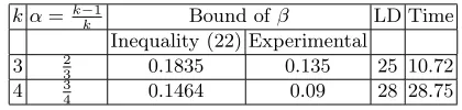
However, we get results in such situations using the results of Section 3. In Table 5, we present few such examples.
k α=k−1
k Bound ofβ LD Time
Inequality (22) Experimental
3 2
3 0.1835 0.135 25 10.72
4 3
4 0.1464 0.09 28 28.75
Table 5.Experimental results for 1000-bita(0)i .
To conclude this section, we like to point out the following issues.
– The method of this section works better than the idea of Section 3 experimentally for larger values of k.
– There are some situations for small values of k, where the idea of Section 3 works better than the strategy in this section.
5
EGACDP
So far we have concentrated on EPACDP, i.e., we considered that the first item is exactly known. However, the more general problem is when the first item is also not known exactly and some approximation is available. This is what we study in this section and we like to refer to EGACDP (see Definition 2). Towards solving EPACDP, we presented two different techniques, one in Section 2 and another in Section 4. We will try similar methods in this section as Method I and Method II respectively. In EGACDP, we have,
a(0)1 = gq1−x(0)1 ,
a(0)2 = gq2−x(0)2 , . . . ,
a(0)k = gqk−x
(0)
k ,
where a(0)1 , . . . , a(0)k are known. We want to find g froma(0)1 , . . . , a(0)k .
5.1 Method I
Towards solving the EGACDP in a manner similar to Section 2, consider the polynomials
h1(x1, x2, . . . , xk) = a
(0) 1 +x1,
. . . ,
hk(x1, x2, . . . , xk) = a(0)k +xk, (23)
wherex1, x2, . . . , xkare the variables. Clearly g(of Definition 2) divides hi(x(0)1 , x (0) 2 , . . . , x
(0)
k )
for 1≤ i≤k.
Now let us define the shift polynomials
hs1,...,sk(x1, x2, . . . , xk) = h
s1
1 . . . h
sk
k , (24)
for non-negative integers u, m such that u≤s1+. . .+sk ≤ m where the integers u, m ≥0
are fixed.
LetX1, . . . , Xk be the upper bounds ofx(0)1 , . . . , x (0)
k respectively. Now we define a lattice
L using the coefficient vectors of h...(x1X1, . . . , xkXk). Let the dimension of L be ω. One
gets x(0)1 , . . . , x(0)k (under Assumption 1 and following Lemma 1 and Lemma 2) using lattice reduction over L, if det(L)ω1 < gm, i.e., when det(L) < gmω (neglecting the lower order
Since the lattice dimension ω=
m
X
s=u
k+s−1
s
is exponential in k, the running time of
this strategy will be poly{loga1,exp(k)}. Thus, for small fixedk this algorithm is polynomial in loga1. To summarize we get the following result.
Theorem 7. Under Assumption 1, the EGACDP can be solved in poly{loga1,exp(k)}time
when det(L)< gmω.
Since in this case matrix corresponding to the LatticeLis not square, finding det(L) may not be easy for generalk. Further, for largek, dimension ofLwill be very large. Experimental results corresponding to this idea are presented in Table 6.
5.2 Method II
Here we follow the idea of Section 4. We have
a(0)1 = gq1−x(0)1 , a(0)2 = gq2−x(0)2 ,
. . . ,
a(0)k = gqk−x(0)k ,
where a(0)1 , . . . , a(0)k are known and a(0)i ≈ a for 1 ≤i ≤k. Suppose, x(0)i ≈ aβ for 1≤ i ≤k
and g ≈a1−α. Then q
i ≈aα fori∈ [1, k].
LetM =
2ρ a(0)
2 a (0)
3 . . . a (0)
k
0 −a(0)1 0 0 0
. . . . . . . .−a(0)1
, where 2ρ ≈2x(0)
1 . One can note that (q1, q2, . . . , qk)·
M = (2ρq
1, x(0)1 q2−q1x(0)2 , . . . , x (0)
1 qk−q1x(0)k ) =b, say.
It can be checked that
||b||<2√kaα+β. (25) Moreover, |det(M)| = 2ρ(a(0)
1 )k−1 ≈ 2aβ+k−1. Following Minkowski’s theorem, there is a vector v in the lattice L corresponding to M such that
||v||<√k21ka β+k−1
k . (26)
Under Assumption 2 (Section 4), and from (25), (26), one can obtain b from L if
aα+β < aβ+kk−1,
neglecting the terms 2 and 2k1; from which we get β < 1− k
k−1α. With the knowledge of
b, one can find q1, from which g is obtained if x(0)1 ≤ q1. So we need 1− k−k1α ≤ α, i.e.,
α ≥ k−1
2k−1. The running time is determined by the time to calculate a shortest vector in L which is polynomial in loga but exponential ink.
Theorem 8. Consider EGACDP with g ≈ a1−α
1 and x (0) 1 ≈ x
(0)
2 ≈ . . . ≈ x (0)
k ≈ a β
1. Then,
under Assumption 2, one can solve EGACDP in poly{loga,exp(k)} time when,
β <1− k
k−1α, (27)
provided α≥ k−1 2k−1.
5.3 Experimental Results
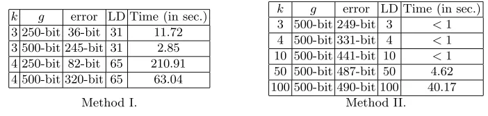
In this section we present a few experimental results for both the methods. When k = 3 and 1−α = 0.25, we have 1− k
k−1α <0. In such a situation one can not get results using Method II, but the Method I will succeed. As example, Method I succeeds given 250-bit g
for k = 3,4, whereas Method II does not provide results in such a scenario.
For large values of k, we can not perform experiments corresponding to Method I due to high lattice dimensions. The statement of Theorem 8 states that the time complexity is poly{loga,exp(k)}. However, under the assumption that “the shortest vector of the latticeL
can be found by the LLL algorithm”, the complexity becomes poly{loga, k}. Thus, Method II will work successfully and we can easily obtain the experimental results using LLL up to
k ≤100.
k g error LD Time (in sec.) 3 250-bit 36-bit 31 11.72 3 500-bit 245-bit 31 2.85 4 250-bit 82-bit 65 210.91 4 500-bit 320-bit 65 63.04
k g error LD Time (in sec.) 3 500-bit 249-bit 3 <1 4 500-bit 331-bit 4 <1 10 500-bit 441-bit 10 <1 50 500-bit 487-bit 50 4.62 100 500-bit 490-bit 100 40.17
Method I. Method II.
Table 6.Experimental results for 1000-bita(0)i .
6
Conclusion
In this paper we present a generalization of the partially approximate common divisor prob-lem (PACDP) [HOW01] which we term as Extended Partially Approximate Common Divisor Problem (EPACDP). This problem immediately relates to the implicit factorization problem introduced in [MAY09]. We consider the case when some MSBs or LSBs or MSBs and LSBs together of the primesp1, p2, . . . , pk are equal (but unknown). This covers the case when the
LSBs are equal (but unknown) in [MAY09] and MSBs are equal (but unknown) in [FAU10]. Our strategy provides new and improved theoretical as well as experimental results. We also study the extension of GACDP (General Approximate Common Divisor Problem) [HOW01]. Here we did not concentrate on the case when some portions of the bits at the middle of p1, p2, . . . , pk are same. This problem has been discussed in [SAR09,FAU10]. However, it
References
[COP97] D. Coppersmith. Small Solutions to Polynomial Equations and Low Exponent Vulnerabilities. Journal of Cryptology, 10(4):223–260, 1997.
[COR07] J. -S. Coron and A. May. Deterministic polynomial-time equivalence of computing the RSA secret key and factoring. Journal of Cryptology, 20(1):39–50, 2007.
[DJK09] M. v. Dijk, C. Gentry, S. Halevi and V. Vaikuntanathan. Fully Homomorphic Encryption over the Integers. Proceedings of Eurocrypt 2010, To be published in Lecture Notes in Computer Science, Springer, 2010. Cryptology ePrint Archive, Report 2009/616, Available at http://eprint.iacr.org/2009/616.
[FAU10] J. -C. Faugere, R. Marinier and G. Renault. Implicit Factoring with Shared Most Significant and Middle Bits. Proceedings of PKC 2010, To be published in Lecture Notes in Computer Science, Springer, 2010. [HOW97] N. Howgrave-Graham. Finding Small Roots of Univariate Modular Equations Revisited. Proceedings of
Cryptography and Coding, Lecture Notes in Computer Science, Volume 1355, pages 131–142, Springer, 1997.
[HOW01] N. Howgrave-Graham. Approximate integer common divisors. Proceedings of CALC 2001, Lecture Notes in Computer Science, Volume 2146, pages 51–66, Springer, 2001.
[ELN07] E. Jochemsz. Cryptanalysis of RSA Variants Using Small Roots of Polynomials. Ph. D. thesis, Technische Universiteit Eindhoven, 2007.
[LLL82] A. K. Lenstra, H. W. Lenstra and L. Lov´asz. Factoring Polynomials with Rational Coefficients. Mathe-matische Annalen, 261:513–534, 1982.
[MAY03] A. May. New RSA Vulnerabilities Using Lattice Reduction Methods. PhD thesis, University of Paderborn, 2003.
[MAY09] A. May and M. Ritzenhofen. Implicit factoring: on polynomial time factoring given only an implicit hint. Proceedings of PKC 2009, Lecture Notes in Computer Science, Volume 5443, pages 1–14, Springer, 2009. [RGV04] O. Regev. Lattices in Computer Science (Lecture Notes), 2004. Available at:
http://www.cs.tau.ac.il/˜ odedr/teaching/lattices fall 2004/index.html [last accessed December 19, 2009]. [RSA78] R. L. Rivest, A. Shamir and L. Adleman. A Method for Obtaining Digital Signatures and Public Key
Cryptosystems. Communications of ACM, 21(2):158–164, February 1978.
[SAR09] S. Sarkar and S. Maitra. Further Results on Implicit Factoring in Polynomial Time. Advances in Mathe-matics of Communications, 3(2):205–217, 2009.
[SAR10] S. Sarkar and S. Maitra. Approximate Integer Common Divisor Problem relates to Implicit Factorization. All the versions available at http://eprint.iacr.org/2009/626. Submitted: 18 Dec 2009, 1st revision: 11 Feb 2010, 2nd revision: 11 May 2010.
![Fig. 1. Comparison of our theoretical result [case (i), works for both MSBs and LSBs] with that of [MAY09] [case(ii), works for LSBs], [FAU10] [case (ii), works for MSBs] and [SAR09] [case (iii), works for MSBs].](https://thumb-us.123doks.com/thumbv2/123dok_us/1863264.1242171/8.612.111.494.287.474/comparison-theoretical-result-works-works-works-works-msbs.webp)
![Table 1. For 1000 bit N, theoretical and experimental data of the number of shared LSBs in [MAY09] and sharedLSBs in our case](https://thumb-us.123doks.com/thumbv2/123dok_us/1863264.1242171/13.612.147.467.460.548/table-theoretical-experimental-data-number-shared-lsbs-sharedlsbs.webp)
![Table 2. For 1024 bit N, theoretical and experimental data of the number of shared MSBs in [FAU10] and sharedMSBs in our case.](https://thumb-us.123doks.com/thumbv2/123dok_us/1863264.1242171/14.612.151.461.248.350/table-theoretical-experimental-data-number-shared-msbs-sharedmsbs.webp)
![Table 3. For 1000 bit N, theoretical (same bound for [MAY09] and in our case) and experimental data of the numberof shared LSBs in [MAY09] and shared LSBs in our case.](https://thumb-us.123doks.com/thumbv2/123dok_us/1863264.1242171/16.612.150.465.344.509/table-theoretical-bound-experimental-numberof-shared-lsbs-shared.webp)