Quantification of Surface Roughness of Lava Flows on Mars

(1)

Western University Western University

Scholarship@Western

Electronic Thesis and Dissertation Repository

12-6-2019 10:30 AM

Quantification of Surface Roughness of Lava Flows on Mars

Carolina Rodriguez Sanchez-Vahamonde

The University of Western Ontario

Supervisor Neish, Catherine

The University of Western Ontario Graduate Program in Geology

A thesis submitted in partial fulfillment of the requirements for the degree in Master of Science © Carolina Rodriguez Sanchez-Vahamonde 2019

Follow this and additional works at: https://ir.lib.uwo.ca/etd

Part of the Geology Commons, Other Earth Sciences Commons, Tectonics and Structure Commons,

The Sun and the Solar System Commons, and the Volcanology Commons

Recommended Citation Recommended Citation

Rodriguez Sanchez-Vahamonde, Carolina, "Quantification of Surface Roughness of Lava Flows on Mars" (2019). Electronic Thesis and Dissertation Repository. 6754.

https://ir.lib.uwo.ca/etd/6754

This Dissertation/Thesis is brought to you for free and open access by Scholarship@Western. It has been accepted for inclusion in Electronic Thesis and Dissertation Repository by an authorized administrator of

(2)

i

Abstract

Volcanism has played a significant role throughout Mars’ geologic history. Extensive lava flows are widely spread across Mars’ equatorial region, shaping the surface in a very distinct way. In radar images (at the decimeter scale), these flows are bright, which is a typical characteristic of extremely rough, blocky lava flows seen on Earth. Although the source of the extreme roughness of Martian lava flows is unknown, their surface roughness parameters can be constrained to 1) gain information about Mars’ interior processes, 2) find appropriate analogues on other planetary bodies, and 3) ideally infer the emplacement style of such lavas. Here, we utilized very detailed high-resolution images of Mars to measure the surface roughness parameters of Martian lava flows at a scale never before examined on the Martian surface (meter scale). Our results determined that at the meter scale, Martian lava flows are smoother than blocky flows seen on Earth, somewhat similar to pāhoehoe and rubbly flows seen in Hawaii and Iceland (which are smooth at the decimeter scale), and similar to young lunar lava flows (also smooth at the decimeter scale). The differences observed in the surface roughness of Martian lava flows at the decimeter and meter scales compared to analogue lava flows on Earth and the Moon might be the result of: 1) the differences in the emplacement style of the lava flows, 2) the differences in post-emplacement modification processes on the surface of the lava flows, and/or 3) the limitations of the technique used to characterize the lava flows.

Keywords

(3)

ii

Summary for Lay Audience

(4)

iii

Co-Authorship Statement

(5)

iv

Acknowledgments

(6)

v

List of Tables

Table 1.1: Types of magma found on Earth with their corresponding characteristics (Winter, 2010). ... 5

Table 1.2: Characteristics of common volcanoes seen on Earth (Earle, 2019). ... 6

Table 1.3: Description and roughness of common lava flows morphologies found on Earth (Kuntz et al., 2007; Guilbaud et al., 2005; Duraiswami et al., 2008; Keszthelyi et al., 2000; Sehlke et al., 2014; Tolometti et al., 2019, submitted). ... 8

Table 2.1: The characteristics of the HiRISE instrument at a 300km altitude (McEwen et al., 2007). ... 27

Table 3.1: HiRISE Digital Terrain Models processed by the HiRISE team in SOCET SET and utilized in this project. Radar-dark DTMs are bolded. ... 41

Table 3.2: HiRISE stereo-pairs processed into digital terrains models using the Ames Stereo Pipeline software. Radar-dark DTMs are bolded. ... 41

Table 3.3: Detailed description of the PDS product naming convention for HiRISE DTMs (https://www.uahirise.org/dtm/about.php; last accessed 18.09.2019). ... 42

Table 3.4: Elevation variations (minimum, maximum, and standard deviation) of ASP and SOCET SET derived DTMs and the elevation difference map derived from these two DTMs. ... 42

Table 3.5: Average RMS slope (Cs) and Hurst exponent (H) extracted for each lava flow region examined in this work. These were extracted in 100 m long topographic profiles from left to right (expressed as Cs and H) and top to bottom (expressed as CsY and HY). ... 46

(10)

ix

(11)

x

List of Figures

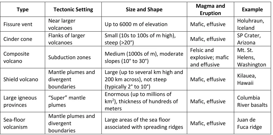
Figure 1.1: Different settings of volcanism on Earth showing different volcanic features formed in different areas (Earle, 2019). ... 3

Figure 1.2: Different types of volcanism on occurring on Earth. A) fissure vent, B) cinder cone volcano, C) shield volcano, D) composite volcano (USGS), E) Large Igneous Province (Bass, W., 2017), F) Pillow lavas formed by sea floor volcanism (D. Kelley/University of Washington). ... 6

Figure 1.3: Different types of lava flow morphologies found on Earth. A) smooth pāhoehoe, B) hummocky Pāhoehoe, C) rubbly Pāhoehoe, D) slabby Pāhoehoe, E) `a`ā flow, F) blocky flow (A_USGS,B, C, E, F_{G. Tolometti,}D_{Neish et al., 2017). ... 9}

Figure 1.4: True color image of Mars taken with the OSIRIS instrument onboard the European Space Agency (ESA) Rosetta spacecraft. ... 10

Figure 1.5: Diagram showing the geologic activity of Mars through time (Modified from: Carr and Head, 2010). ... 14

Figure 1.6: MOLA (Mars Orbiter Laser Altimeter) shaded relief map (Smith et al., 2001), showing the location of the 24 major volcanoes on Mars (Robbins et al., 2011). ... 16

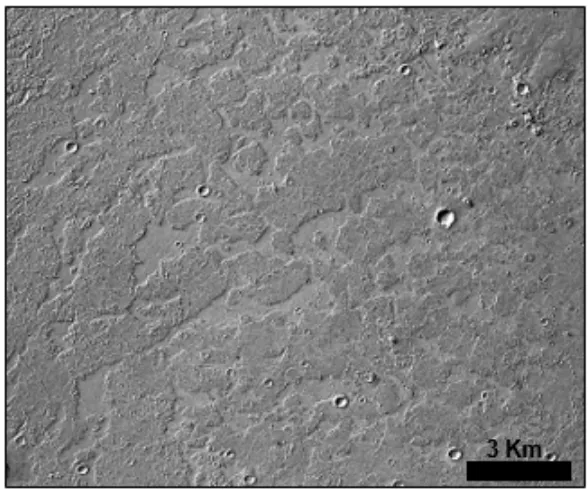
Figure 1.7: A Context Camera image (B19_017097_1541) taken from the Mars Reconnaissance Orbiter spacecraft, showing a platy ridge flow texture located in the Tharsis volcanic region of Mars. ... 17

(12)

xi

Figure 1.9: Diagram showing how the roughness of a planetary surface affects the Circular Polarization Ratio (Neish and Carter, 2014). ... 20

Figure 1.10: (Top) Arecibo radar image of Mars at 12.6 cm wavelength (S-band). Terrains with bright radar returns represent the volcanic regions of the planet (i.e., Elysium, Marte Vallis, Tharsis) (Harmon et al., 2012). (Bottom) Optical global map of Mars (http://www.planetary.brown.edu/planetary/rough/) taken with the Mars Orbiter Camera instrument onboard the Mars Global Surveyor Spacecraft. North is up in both images. . 22

Figure 1.11: Arecibo circular polarization ratio image of Mars at 12.6 cm wavelength (S-band) (Harmon et al., 2012). ... 22

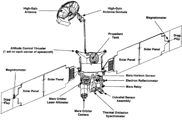
Figure 2.1: A sketch of NASA’s MRO spacecraft labeling its scientific and engineering instruments (Taylor et al., 2014). ... 25

Figure 2.2: Sketch of the HiRISE instrument with the MRO support ring showing its main devices (focal plane electronics, power supply, and remote electronics) on the back of the telescope (McEwen et al., 2007). ... 27

Figure 2.3: Drawing of a CCD push broom scanning motion in a satellite (Campbell, 2007). ... 28

Figure 2.4: Sketch of (a) the CCD array in the focal plane subsystem of the HiRISE instrument, and (b) reference data on every Detector Chip Assembly (DCA). Each DCA is made of a CCD and a Computer Processing Memory Module (CPMM). Here the motion of the MRO spacecraft is looking down (McEwen et al., 2007). ... 28

Figure 2.5: A sketch of the Mars Global Surveyor spacecraft showing its instruments and major components (Albee et al., 2001). ... 29

Figure 2.6: Global Map of the TES Dust Cover Index on top of the Mars Orbiter Laser Altimeter shaded relief base map (NASA/JPL/Goddard). ... 31

(13)

xii

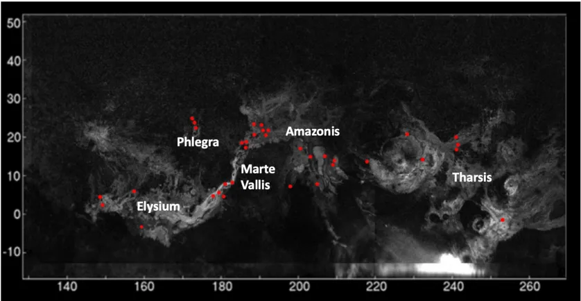
Figure 2.8: Radar backscatter image of Mars showing the areas where the HiRISE stereo pairs were processed into DTMs. Number located at the edges of the map represent the latitude and longitude coordinates. Modified from: (Harmon et al., 2012) ... 33

Figure 2.9: Workflow to create a HiRISE Digital Terrain Model using Ames Stereo Pipeline (Beyer et al., 2018). ... 34

Figure 2.10: Topographic profile of a smooth Martian lava flow located in the Tharsis volcanic region. The topographic profile was extracted from the HiRISE DTM: DTEED_045395_1980_045817_1980_Z01. ... 36

Figure 2.11: A variogram plot of a smooth lava flow located in the Tharsis region of Mars. The Points are plotted every 2 meters between 2 meters and 12 meters (the baseline utilized in this work). The Hurst exponent is the slope of the line and the RMS is related to the y-intercept. ... 37

Figure 2.12: (A) HiRISE image (ESP_045395_1980) of a smooth lava flow located on the Tharsis volcanic region of Mars. Black outline represents the area in which the Hurst exponent and the RMS slope were calculated. (B) DTM of the region of study. Red line represents the first row in which these parameters are being calculated. (C) Hurst exponent and (D) RMS slope results of the entire portion of the lava flows. ... 37

Figure 2.13: (Left) The MGS-TES DCI map over the MRO-MOLA shade-relief global map of Mars. The black box represent the HiRISE image of the volcanic feature studied. (Right) Close up image of the area of interest showing the custom shape files created (inside the HiRISE image) to extract the DCI parameters of two lava flow portions. North is up in all images. ... 38

(14)

xiii

Figure 3.2: RMS slope (Cs) versus Hurst exponent (H) for the Martian lava flows we analyzed, divided into five different regions: Amazonis (red), Elysium (orange), Marte Vallis (yellow), Phlegra (green), and Tharsis (blue). ... 45

Figure 3.3: RMS slope versus Hurst exponent for the Martian lava flows analyzed in this study, divided into radar-bright (red) and radar-dark (orange) volcanic surfaces. ... 45

Figure 3.4: RMS slope versus TES Dust Cover Index for the Martian lava flows analyzed in this study, divided into radar-bright and radar-dark volcanic surfaces. ... 47

Figure 3.5: (A) MRO context image (G18_025207_1976_XI_17N150W) of a lava flow covered in dust on Mars. Black box in image shows the portion of the surface used to calculate the Hurst Exponent and the RMS slope of the lava flow. North is up in this image (B) Close up of a HiRISE image of the region of interest. (C) Hurst Exponent and (D) RMS slope calculated from left to right for this region. (E) Hurst exponent and (F) RMS slope calculated from top to bottom for this region. (G) DTM of the region of interest (E = elevation from spacecraft), and (H) TES DCI of the surface. ... 49

Figure 3.6: (A) MRO context image (G16_024_587_1465_XN) of a relatively dust-free lava surface on Mars. Black box in image shows the portion of the surface used to calculate the Hurst Exponent and the RMS slope of the lava flow. (B) Close up of a HiRISE image of the region of interest. (C) Hurst Exponent and (D) RMS slope calculated from left to right for this region. (E) Hurst exponent and (F) RMS slope calculated from top to bottom for this region. (G) DTM of the region of interest, and (H) TES DCI map of Mars over the HiRISE image of the region. North is up in all images. ... 50

Figure 4.1: (Left) Optical image (ESP_026461_2080) and (Right) Arecibo radar backscattered image of a Martian flow observed to be smooth at the meter scale and decimeter scale (Harmon et al., 2012). ... 55

(15)

xiv

Figure 4.3: (Left) HiRISE image (ESP_013249_1805) and (Right) Arecibo radar backscattered image of a Martian flow observed to be rough at the meter scale and smooth at the decimeter scale (Harmon et al., 2012). ... 56

Figure 4.4: (Top) UAVSAR-L-Band CPR image of Sabancaya lava flow in Peru (C. Neish). (Bottom) Sabancaya as seen with optical imagery from the International Space Station (NASA) ... 57

Figure 4.5: RMS slope and Hurst Exponent parameters at the meter scale derived from this work (upper plot) and Neish et al. 2017 (lower plot) for the Earth and Moon. ... 58

Figure 4.6: Image of the lunar crater Gerasimovich D (far side of the Moon) as seen at (a) optical wavelengths by the LRO wide-angle camera, and (b) radar wavelengths (S-Band: 12.6 cm) by Mini-RF instrument onboard the LRO spacecraft. Note that the impact melt flow (white arrow) is not easily observed in image (a) but is visible in image (b) due to the radar’s sensitivity to buried, rough surfaces. From: (Neish et al., 2014) Here, the flow is buried by lunar regolith, rather than Martian dust. ... 61

(16)

xv

List of Appendices

(17)

1

Chapter 1

1 Introduction

Mars has been of particular interest to the planetary science community for decades as it is the only planetary body, besides Earth within the habitable zone of our Solar System. Evidence of flood lavas and massive volcanoes suggests that volcanism on Mars has played a significant role throughout its entire geologic history. Extensive lava flows are spread widely across Mars’ equatorial region, shaping the surface in a very distinct way (Keszthelyi, et al., 2000; 2004; 2006). On radar images (at the decimeter scale), these surfaces are observed to be extremely rough (Harmon et al., 2012), which produce radar bright signal returns; a typical characteristic of blocky lavas flows seen on Earth (Neish et al., 2017). The source of such extreme roughness for Martian lava flows has not yet been identified. However, we can measure and constrain its roughness at different scales using high-resolution datasets of Mars that have been acquired over the years from different Mars spacecraft missions (McEwen et al., 2007).

Surface roughness can be defined as the topographic expression of a surface over different horizontal scales (i.e., centimeters, meters, kilometers) (Shepard et al., 2001). Planetary scientists often measure the surface roughness of lava flows at different scales on different planetary bodies as they give clues about the emplacement style of the lava flows and the interior processes of the planetary body being studied. Here, we measure the surface roughness of Martian lava flows because 1) in radar data, Martian lava flows are extremely rough in comparison with most other lava flows in the solar system (Harmon et al., 2012); and 2) Mars has very detailed high-resolution topographic datasets (1 - 2m for HiRISE) which allows us to quantify the roughness of large regionsat a scale never before attempted on the Martian surface (McEwen et al., 2007).

(18)

2

1.1 Volcanism

Volcanism is a fundamental geologic process that has played a significant role in the formation and evolution of the solid bodies of our Solar System. It can be defined as the process in which molten rock (magma), pyroclastic fragments, steam, and/or hot water reach the surface of a solid body from its interior. On Earth, volcanism occurs in three different geologic settings: 1) divergent boundaries, 2) convergent boundaries, and 3) mantle plumes / hot spots (see Figure 1.1; Francis and Oppenheimer, 2004; Earle, 2019; Winter, 2010). These three systems work in different ways and produce different types of volcanic features (i.e., eruption and volcano styles, lava flows) which will be briefly explained in the following subsections.

1.1.1 Tectonic Settings of Volcanism on Earth

1.1.1.1 Divergent Boundaries

A divergent plate boundary, also known as constructive boundary, is a tectonic boundary in the lithosphere where two adjacent plates diverge and magma flows upward to fill the gap, creating new sea crust (see Figure 1.1; Earle, 2019; Winter, 2010). On Earth, divergent boundaries form submarine mountain chains, “mid-ocean ridges”. These mountainous features extend roughly 65,000 km long, expand 2,000 km wide, and reach 1 to 3 km in height. Divergent plates boundaries can occur in both ocean settings and within continents. When they occur in the ocean, they create new sea crust, and when within continents, they separate continents and/or generate rift valleys (Winter, 2010).

1.1.1.2 Convergent Boundaries

(19)

3

continental-continental boundaries, where the two boundaries push against each other, generating folds, faults and chains of mountains of uplifted rocks in land. The volcanic rocks formed in these three different setting differ from one another, as their magma composition varies (see Section 1.1.2; Earle, 2019; Winter, 2010). An ocean-ocean convergent boundary, for example, will mainly form basaltic volcanic rocks, while an ocean-continental convergent boundary will form basaltic-andesitic volcanic rocks. Magma, however, is unable to penetrate the thick crust of a continental-continental boundaries, so it cools and metamorphoses intrusively, forming granite and gneiss (Earle, 2019).

1.1.1.3 Mantle Plumes - “Hot Spots”

A mantle plume is defined as an ascending column of hot rock that emanates from the mantle (see Figure 1.1). At the base of the lithosphere the mantle plume undergoes partial melting, forming mafic magma that eventually rises onto the surface of the planet forming volcanic eruptions. As the tectonic plate moves over the stationary hot spot, the volcanoes are rafted away and new ones form in their place. This results in chains of volcanoes, such as the Hawaiian Islands (Earle, 2019; Winter, 2010).

(20)

4

1.1.2 Magma Composition and Eruption Style

As alluded to above, the composition of a magma varies with tectonic setting. At divergent oceanic boundaries and mantle plumes, for example, the magma will tend to be mafic in composition as there is little to no interaction with crustal materials and magma fractionation to form felsic melt. At subduction zones, on the contrary, the magma will tend to be more felsic and alkaline in composition, as it will be able to rise through the crust, creating an interaction between the magma itself and the crustal rock (Francis and Oppenheimer, 2004; Earle, 2019; Winter, 2010).

The properties of a magma depend on its 1) chemical composition (i.e., silica and alkaline content); 2) volatile content, which are components that behave as gases in a volcanic eruption such as water (H2O), carbon dioxide (CO2), and Sulphur dioxide (SO2); and 3)

temperature, which ranges from 800°C to 1200°C (a value linked to its chemical composition). Felsic magmas are rich in silica and volatile content, and are produced at low temperature, resulting in high viscosity magmas (see Table 1.1; Winter, 2010). Conversely, mafic magmas are silica poor, have low levels of volatiles, and are produced at high temperature, resulting in low viscosity magmas (see Table 1.1; Winter, 2010). There are, however, magmas with intermediate compositions that have intermediate silica and volatile contents, and are produced at intermediate temperatures which generate magmas with intermediate viscosities (see Table 1.1). The most common volatiles found in magmas are H2O, CO2, and SO2 (Earle, 2019).

(21)

5

Magma type SiO2 _{Temperature (◦C)}Eruption Viscosity Gas Content Eruption Style

Mafic ~50% ~1100 Low Low Effusive

Intermediate ~60 % ~1000 Intermediate Intermediate Intermediate

Felsic ~70% ~800 High High Explosive

Table 1.1: Types of magma found on Earth with their corresponding characteristics (Winter, 2010).

1.1.3 Types of Volcanoes

On Earth, there are different types of volcanoes that are formed at different tectonic settings. They vary in shape, size, magma composition, eruption style, and produce different types of lava flows. In this section, we briefly mention and describe the most common types of volcanoes seen on Earth (see also Table 1.2).

Fissure vents are fractures near a volcano where mafic lava rises to the surface (see Figure 1.2). Cinder cones are also small volcanoes that are often found at the flanks of large volcanoes. They are monogenic (i.e., formed by one single eruption) small-size volcanoes (up to hundreds of meters high) made up of fragments of vesicular mafic rock (i.e., scoria). Such vesicular loose fragments make these volcanoes easy to erode as they have little strength (see Figure 1.2). Composite volcanoes, on the other hand, are medium-size volcanoes (up to thousands of meters high) formed at subduction plate boundaries. They typically produce intermediate magmas, but their magma composition may vary from felsic to mafic (see Figure 1.2). Large-size volcanoes on Earth include shield volcanoes, which can go up to several km high and hundreds of km across and have gentle slopes (2° to 10°). They are formed, however, at mantle plumes and divergent boundaries and produce mafic magmas (see Figure 1.2). Large igneous provinces (i.e., the 160, 000 km2_{Columbia River}

(22)

6

Type Tectonic Setting Size and Shape Magma and _Eruption Example

Fissure vent Near larger

volcanoes Up to 6000 m of elevation Mafic, effusive

Holuhraun, Iceland Cinder cone Flanks of larger _volcanoes Small (10s to 100s of m high), _{steep (>20°)} Mafic, effusive SP Crater, _Arizona

Composite

volcano Subduction zones Medium (1000s of m), moderate slopes (10° to 30°)

Felsic and explosive; mafic and effusive Mt. St. Helens, Washington Shield volcano

Mantle plumes and divergent

boundaries

Large (up to several km high and 200 km across), not steep

(typically 2° to 10°) Mafic, effusive

Kilauea, Hawaii Large igneous provinces “Super” mantle plumes

Enormous (up to millions of km2_{), thickness of hundreds of}

meters Mafic, effusive

Columbia River basalts

Sea-floor volcanism

Mantle plumes and divergent

boundaries

Large areas of the sea floor

associated with spreading ridges Mafic, effusive Juan de Fuca ridge

Table 1.2: Characteristics of common volcanoes seen on Earth (Earle, 2019).

(23)

7

1.1.4 Lava Flows

Lava flows are streams of molten rock that emanate from a volcano. They have different compositions that range from basaltic (low viscosity), to andesitic (intermediate viscosity), to dacitic and rhyolitic (high viscosity), that lead to different lava flows morphologies (Francis and Oppenheimer, 2004). Their physical properties also depend on their emplacement style and the cooling environment in which they were emplaced (Francis and Oppenheimer, 2004).

Basaltic flows (low viscosity) generate two primary lava flows morphologies: 1) à`ā, and 2) pāhoehoe. An à`ā flow consists of two distinct zones: 1) an upper rubbly zone, and 2) a lower zone of solidified lava that cooled down slowly, isolated by the upper zone. Centimeter-size vesicles are normally present within this type of lava flow, making this morphology rough at the decimeter and at the meter scale (see Table 1.3; Francis and Oppenheimer, 2004). Pāhoehoe flows, on the other hand, may generate different surface textures as they flow across a surface. Some of the textures that they form are: smooth pāhoehoe: smooth glassy surfaces; shelly pāhoehoe: smooth surfaces composed of thin shells that break easily when disturbed; hummocky pāhoehoe: undulating, smooth surfaces; rubbly pāhoehoe: brecciated surfaces composed of broken rubble; slabby pāhoehoe: broken surfaces composed of slabs of the originally smooth pāhoehoe flow (see Table 1.3; Francis and Oppenheimer, 2004; Neish et al., 2017). Each of these surface textures present different roughness at multiple scales, which are shown in Table 1.3 (Glaze & Baloga, 2007; Glenn et al., 2006; Rosenburg et al., 2011; Whelley et al., 2017; 2014). Pāhoehoe and à`ā flows have similar chemical compositions and they may even emanate from the same vent. À`ā, flows are typically formed at higher effusion rates (i.e., 5-10 m3_s-1 _in

Hawaii) than pāhoehoe flows (Rowland and Walker, 1990), and are also present in some andesitic flows. A pāhoehoe may transition to an`a`ā when the lava flow encounters a steep slope, as a response to sudden changes in the shearing stress of the flow, and in turn, may transition back to a pāhoehoe at shallow slopes (Francis and Oppenheimer, 2004).

(24)

8

“blocky” lava flows, typically consist of decimeter to meter-size angular blocks laying on top of one another on the surface of the lava flow, resulting in a high roughness at the decimeter to meter scale and low roughness at other scales (i.e., the rough surface texture will be indistinguishable at smaller scales (see Table 1.3). Blocky lava flows are usually andesitic flows, however, they can also form in dacitic lava flows. Dacitic flows, however, have higher viscosities and yield strength than those types of lava discussed above (basaltic and andesitic). They usually form thick, steep, crystal-rich (~50%) extrusions, usually referred as “lava domes”. A less common lava flow found on Earth are rhyolitic lava flows, which are found within calderas, where they form extrusions similar to dacitic flows. However, they form rocks of pure glass (i.e., obsidian) rather than rocks with phenocrysts, as seen in dacitic flows (Francis and Oppenheimer, 2004).

Lava Flow Morphology Description Roughness

Smooth Pāhoehoe A smooth lava flow with a _{thin, glassy crust.} Smooth at cm- and m-scales

Hummocky Pāhoehoe Undulating pāhoehoe lava. Smooth at km-scales; Rough at cm- and m-scales due to hummocks

Rubbly Pāhoehoe

A lava flow with a preserved flow base and brecciated

pāhoehoe crust. Rough at m and dm-scales

Slabby Pāhoehoe Fractured slabs of pāhoehoe _crust. Smooth at cm-scales; Rough _{at m- and km-scales}

`A`ā Lava flow with a rough _{clinkered surface.} Rough at m and dm-scales

Blocky Lava flows composed of dm _{to meter-size blocks} Smooth at cm-scale; Rough at _{dm- and m-scales}

(25)

9

Figure 1.3: Different types of lava flow morphologies found on Earth. A) smooth pāhoehoe, B) hummocky Pāhoehoe, C) rubbly Pāhoehoe, D) slabby Pāhoehoe, E) `a`ā flow, F) blocky flow (A_USGS,B, C, E, F_{G. Tolometti,}D_{Neish et al., 2017).}

1.2 Mars

1.2.1 The Geologic History of Mars

(26)

10

volcanism, impact cratering, erosion, and aeolian and atmospheric processes. The red-colored appearance of its soil is due to iron minerals that have undergone oxidation (see Figure 1.4; Carr and Bell, 2014). Mars has a thin atmosphere composed of CO2, nitrogen

(N2), argon (Ar), and small amounts of water vapor and oxygen (Carr and Bell, 2014).

Several orbiting and lander/rover missions has been sent to Mars to study the planet in detail, as it is the only other planet within the habitable zone of our Sun besides Earth (Carr and Bell, 2014). These missions have provided us with invaluable information about Mars geologic history, which we briefly discuss in this section.

The geology of Mars is dominated by the dichotomy between the smooth northern plains and heavily cratered southern highlands (Frey and Schultz, 1988; Lenardic et al., 2004; McGill & Dimitriou, 1990). The geological history of Mars is divided into three periods: Noachian (4.1 - 3.7 Ga), Hesperian (3.7 - 3.0 Ga), and Amazonian (3.0 Ga – Present), which are going to be briefly explained in the following subsections.

(27)

11

1.2.1.1 Pre-Noachian

The pre-Noachian covers the time from Mars’ formation (4.5 Ga) to the formation of the impact basin Hellas (4.1 Ga) (Frey, 2003). During this period the magnetic field, large basins, and Mars’ dichotomy formed (McGill and Squyres, 1991; Nimmo and Tanaka, 2005). Mars’ dichotomy is characterized by differences in elevation, crustal thickness, and crater densities (Aharonson et al., 2001). The difference in elevation at the boundary of the dichotomy is around 5 km (Aharonson et al., 2001), and the thickness of the crust is estimated to be 60 km to the south and 30 km to the north (Neumann et al., 2004). The formation mechanism for the dichotomy is still unknown, but may have been caused by a single giant impact, or a cluster of impact basins (Frey, 2003; Lenardic et al., 2004; McGill & Dimitriou, 1990). However, recent studies support the idea that it was formed by one giant impact (Andrews et al., 2008).

1.2.1.2 Noachian

The Noachian period (4.1 - 3.7 Ga) is mainly characterized for its high rates of cratering, erosion and valley formation, and the formation of Tharsis, the largest volcanic region on Mars (see Figure 1.5; Carr and Head, 2010). Most of the volcanism during this period occurred in Tharsis, which resulted in a large volume of volcanic material being emplaced in and around this region (Philips et al., 2001). On a global scale, the formation of Tharsis led to a deformation of the Martian lithosphere. This created a trough all around the rise of Tharsis, an antipodal rise, and gravity anomalies around Tharsis (Philips et al., 2001). Most Noachian volcanic terrains are covered by younger deposits and cannot been seen (Carr and Head, 2010). However, some of them are exposed as primary and/or deformed volcanic rocks in cratered uplands (Bandfield et al., 2000; Mustard et al., 2005) and are mainly characterized by basalt with low calcium pyroxene and different amounts of olivine (Bibring et al., 2006; Poulet et al., 2005).

(28)

12

Gulick, 1998). Deltas and fans observed in most valleys share similar stream draining to those seen on Earth, such as, Eberswalde crater (Fassett and Head, 2005; Malin and Edgett, 2000; Moore et al., 2003). Chlorine and sulfate rich deposits found within the valleys are the result of the evaporation of lakes and inter-dune lakes (Osterloo et al., 2004; Grotzinger et al., 2005).

The Noachian period is also known for the presence of phyllosilicate minerals all over the planet. These are minerals that are formed by the aqueous alteration of basalts (i.e., saponite, Fe-rich chlorites, nontronite, and montmorillonite). They are observed to be present in olivine-rich rocks, and have also been exposed to the surface by erosion (Mustard et al., 2007). Evidence found in the Noachian terrains (i.e., valleys, phyllosilicates, groundwater sapping) strongly suggests that the surface conditions during this period were consistent with extensive aqueous erosion and the climate was much wetter in comparison to other, younger geologic periods (Bibring et al., 2006; Fassett and Head, 2008; Grotzinger et al., 2005; Carr, 2006; Murchie et al., 2008).

1.2.1.3 Hesperian

The Hesperian period (3.7 - 3.0 Ga) is characterized by continuous and/or periodic volcanism that led to the formation of massive lava plains, and the formation of canyons and extensive outflow channels on the surface of Mars (Hartmann et al., 2001). During this period, the rates of erosion, weathering and valley formation decreased in comparison to the Noachian period (see figure 1.5; Carr and Head, 2010).

(29)

13

Olympus Mons, the largest volcano in our Solar System, and Valles Marineris started to form during the Hesperian period (Head et al., 2002).

The erosion rate of Mars decreased by 2-5 orders of magnitude during this period in comparison to the Noachian (Golombek et al., 2006). The weathering rate also dropped significantly, leading to fewer phyllosilicates and more sulfate-rich deposits in the surface (Bandfield et al., 2000). This drastic climate change resulted in a thick global cryosphere.

1.2.1.4 Amazonian

The Amazonian period (3.0 Ga – Present) covers two thirds of Martian history (Hartmann and Neukum, 2001). Surface processes involving ice and wind are the two main processes operating during this period. The volcanic rates during this period are generally low; in comparison with the Hesperian, the average rate is a factor of ten lower in this period. Most of the volcanic activity took place in Tharsis and Elysium volcanic regions in this period (see Figure 1.5).

(30)

14

Figure 1.5: Diagram showing the geologic activity of Mars through time (Modified from: Carr and Head, 2010).

1.3 Volcanism on Mars

Volcanism has played a significant role throughout Mars’ geologic history. Volcanic features (i.e., mons: large volcanoes; patera: irregular craters; tholi: small mountains; small construct: low shield and fissures; basins, and volcanic plains) are widely spread across Mars’ surface. Mars has four major volcanic regions (Tharsis, Elysium, Syrtis Major, and Hellas) and 24 major volcanoes within these regions, which are briefly described in this section.

1.3.1 Tharsis

(31)

15

Olympus Mons, Ascraeus Mons, Pavonis Mons, and Arsia Mons), and 7 small ones (Ceraunius Tholus, Uranius Tholus, Tharsis Tholus, Jovis Tholus, Biblis Tholus, and Ulysses Tholus), which are shown in Figure 1.6. Its major volcanoes are similar to shield volcanoes seen on Earth but at a much larger scale (Zimbelman et al., 2015). For example, Olympus Mons is 500 km wide and 25 km high, almost three times higher than Mt. Everest on Earth.

1.3.2 Elysium

The Elysium region consists of three volcanoes: Elysium Mons, Hecates Tholus, and Albor Tholus (see Figure 1.6; Robbins et al., 2011). The morphology of Elysium Mons is similar to the central volcanoes located in Tharsis, but with much steeper slopes (up to 12°) (Zimbelman et al., 2015). The lava flows from Elysium Mons exceed 700 km in length and their morphology is also similar to those seen in Tharsis (Keszthelyi et al., 2006).

1.3.3 Syrtis Major and Hellas Basin

(32)

16

Figure 1.6: MOLA (Mars Orbiter Laser Altimeter) shaded relief map (Smith et al., 2001), showing the location of the 24 major volcanoes on Mars (Robbins et al., 2011).

1.3.4 Martian Lava Flows

Flood lavas are extensive lava flows that can cover a large portion of a planetary surface (Geikie, 1880; Washington, 1922; Tyrell 1937). The mode of formation of these flows can be associated with the presence of a mantle plume in the lithosphere of the planet and/or the movement of its continents (Morgan, 1972; White and McKenzie, 1995). The majority of flood lavas are characterized by basalt (Coffin and Eldholm, 1994). On Earth, however, they are also seen to be characterized by more siliceous basaltic andesite (i.e., Columbia River Basalt Group) (Hooper, 1997), as well as dacites and rhyolites (i.e., Etendeka-Paraná flood basalts) (Marsh et al., 2001).

(33)

17

On Mars, flood lavas are basaltic in composition and are seen to be widely spread across the surface (Keszthelyi et al., 2004). Martian flood lavas are typically young (Amazonian age) (Plescia, 1990; Lanagan, 2004), massive (>1500 km) (Lanagan, 2004), and have shallow slopes. They are also observed to be pāhoehoe flows with a “platy-ridge” texture (see Figure 1.7) (Keszthelyi et al., 2000), which is thought to form when surges of lava disrupt a solidified pāhoehoe sheet flow (Keszthelyi et al., 2004). This type of texture is seen in parts of the Laki lava flow in Iceland, the closest terrestrial analogue to Martian flood lavas ever identified (Keszthelyi et al., 2000).

As stated above, the majority of flood lavas on Mars are located near its equatorial region. Some of the youngest and best-preserved Martian flood lavas are observed in Elysium Planitia (Plescia, 1990), Amazonis Planitia (Zimbelman et al., 2015), and Marte Vallis (Zimbelman et al., 2015). The Tharsis region is also home to a large number of Martian flood lavas. Layers of flood lavas are also exposed in the walls of Valles Marineris. These are, however, older than those seen in Elysium, Amazonis, and Marte Vallis (Zimbelman et al., 2015).

(34)

18

1.4 Planetary Radar Remote Sensing

In this work, we utilized RAdio Detection And Ranging (RADAR) datasets of Mars to quantify the surface roughness of Martian lava flows. RADAR is an active remote sensing technique that uses the echo of a radio wave transmission to study the physical and electrical properties of the surface and near surface of a planetary body (see Figure 1.8; Neish and Carter, 2014). There are three main techniques - radar imagery, radar sounding, and radar topography – that can be used to measure different aspects of a planetary surface (Neish and Carter, 2014). Radar imagery uses Doppler shift and time delay to generate two dimensional images of a specific target at centimeter to decimeter scale wavelengths (Harmon et al., 2012; Neish and Carter, 2014). Radar sounding, on the other hand, uses long wavelengths (meters to hundreds of meters) to measure the subsurface structure of an object (Neish and Carter, 2014; Seu et al., 2007). Radar altimeters can be used to measure the topography of a planetary surface. In this work, we utilize radar imagery obtained from the Arecibo Observatory S-Band (12.6 cm) radar.

1.4.1 Surface Properties

The albedo of optical and radar images is sensitive to different surface properties. Optical images detect the light reflected by the surface of a planetary body, which is influenced by its chemical composition. Radar images sense the physical and electrical properties (i.e., change in slope, roughness, dielectric constant) of a planetary surface (Neish and Carter, 2014). Short wavelengths (i.e., 12.6 cm or S-band) are used to measure the roughness of various planetary surfaces (Harmon et al., 2012). This is because different surface roughness values will result in different radar backscatter values. Smooth surfaces result in very low backscatter returns, and rough surfaces result in high backscatter returns (see Figure 1.8; Neish and Carter, 2014; Farr, 1993).

(35)

19

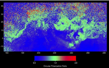
backscatters off an interface, the polarization of such wave will change; as a consequence, smooth surfaces will tend to have high OC returns and low CPR values (0 - 0.4) because the radar wave will only bounce once, flipping its polarization. Moderately rough surfaces, on the other hand, will tend to have equal OC and SC returns and moderate CPR values (0.5-1), because the radar wave will have multiple bounces that will randomize the polarization. Blocky surfaces, however, will have high SC returns and have high CPR values (>1), because the radar wave will reflect in the corners of the surface causing a double bounce backscattering (see Figure 1.9; Neish and Carter, 2014).

(36)

20

Figure 1.9: Diagram showing how the roughness of a planetary surface affects the Circular Polarization Ratio (Neish and Carter, 2014).

1.4.2 Radar Data for Mars

(37)

21

(38)

22

Figure 1.10: (Top) Arecibo radar image of Mars at 12.6 cm wavelength (S-band). Terrains with bright radar returns represent the volcanic regions of the planet (i.e., Elysium, Marte Vallis, Tharsis) (Harmon et al., 2012). (Bottom) Optical global map of Mars (http://www.planetary.brown.edu/planetary/rough/) taken with the Mars Orbiter Camera instrument onboard the Mars Global Surveyor Spacecraft. North is up in both images.

Figure 1.11: Arecibo circular polarization ratio image of Mars at 12.6 cm wavelength (S-band) (Harmon et al., 2012).

1.5 Summary and Aim

(39)

23

silicic, a result of the unique tectonic environment of our home planet. Plate tectonics are not thought to operate on Mars, and most lava flows there are basaltic in composition, which do not typically produce blocky flows. Thus, the unique roughness properties of Martian lava flows have motivated us to further study their physical characteristics. In the process, we hope to 1) gain information about Mars’ interior processes, 2) find appropriate analogues to Martian flows on other planetary bodies, and 3) ideally, infer the emplacement style of such lavas. In this work, we utilized high-resolution images of Mars to measure the surface roughness parameters of these flows at a scale never before examined on the Martian surface (meter scale).

(40)

24

Chapter 2

2 Datasets and Methodology

In this project, we used datasets from: 1) the High-Resolution Imaging Science Experiment (HiRISE) instrument onboard the Mars Reconnaissance Orbiter (MRO) spacecraft, and 2) the Thermal Emission Spectrometer (TES) instrument onboard the Mars Global Surveyor (MGS) spacecraft, to constrain the surface roughness of Martian lava flows. More specifically, we used HiRISE datasets to generate Digital Terrain Models (DTM) of volcanic surfaces on Mars to extract their surface roughness at the meter scale. We also calculated the Dust Cover Index (DCI) derived from MGS-TES datasets for each of the lava flows studied. In the following sections we give details on the datasets utilized and methodology for this work.

2.1 Mars Reconnaissance Orbiter

The NASA MRO is a science mission that has been orbiting Mars since 2006. Its general science objective is to enable our understanding of the evolution of the Martian surface, subsurface and atmosphere through time and to identify potential sites for future landed missions to the planet (Zurek and Smrekar, 2007). To meet these goals, the spacecraft was designed to include six science instruments (three imaging systems, one visible-near infrared spectrometer, one shallow-probing subsurface radar, and one thermal-infrared profiler) that acquire dataof Mars; three engineering instruments that allow the spacecraft to navigate and communicate between Earth, MRO, and landed missions on Mars; and two science-facility experiments that depend on engineering data to map Mars’ gravitational field and understand its atmospheric structure (Zurek and Smrekar, 2007). Figure 2.1 shows the NASA MRO spacecraft with its instruments.

(41)

25

Figure 2.1: A sketch of NASA’s MRO spacecraft labeling its scientific and engineering instruments (Taylor et al., 2014).

2.1.1 High Resolution Imaging Science Experiment Instrument

The NASA MRO HiRISE instrument was designed to acquire very high resolution (25 cm to 1.3 m per pixel) images of the surface of Mars from an altitude of 300 km (McEwen et al., 2007). It mainly consists of 1) a telescope with an aperture of 25 cm, 2) a focal plane subsystem containing 14 Charged Couple Device (CCD) detectors, and 3) two remote electronics boxes for the power supply and instrument controller (see Figure 2.2; McEwen et al., 2007).

(42)

26

color image of the instant field of view in a single swath, while providing a three-color image of a 1.2 km wide swath across the central stripe (see Figure 2.4; McEwen et al., 2007). In 2011, the electronics for the RED-9 CCD, located on the right site of the swath, were lost. This narrowed the swath width of the subsequent images by 10%, rather than creating a gap within the image (McEwen et al., 2018). Table 2.1 provides details on the parameters of the HiRISE instrument.

A HiRISE observation is made of a set of Experiment Data Record (EDR) products for each CCD channel, resulting in a total of 28 EDR products per observation. The generation of such EDR products is: 1) the decompression of the image and accommodation of all data gaps, 2) the organization of the image data by the CCD channel, 3) the extraction of the information needed for the Planetary Data System (PDS) labels, and lastly 4) the organization of additional metadata within the file (McEwen et al., 2007). The size of a single EDR product varies within observations and depends on its commanding parameters (i.e., number of observation lines, pixel binning, and image pixel data type). Typically, the largest file sizes are those observations of highest priority (i.e., landing site assessment campaigns). The majority of the EDR products used in this project are 10 to 80 megabytes in size.

(43)

27

Parameters Characteristics

Ground sampling dimension 30 cm/pixel (1 µrad IFOV) Resolution ~90 cm (3 pixels across an object) Swath width (RED CCDs) 6 km (1.14⸰ FOV)

Color swath width 1.2 km (0.23⸰ FOV)

Maximum image size (pixels) 20,000 x 63,780 (14-bit data) SNR (anywhere on Mars in the optimal

season)

From 90:1 to 250:1 in RED channels with TDI 128 and full resolution

Color band passes RED: 570– 830 nm, BG: <580 nm, NIR: >790 nm Stereo topographic precision ~25 cm vertical over ~1 m² areas

Pixel binning none (1 x 1), 2 x 2, 3 x 3, 4 x 4, 8 x 8, 16 x 16

Bits per pixel 14, can be compressed to 8 via look-up tables (LUTs) Compression (8-bit images only) FELICS, compression >1.6:1

Table 2.1: The characteristics of the HiRISE instrument at a 300km altitude (McEwen et al., 2007).

(44)

28

Figure 2.3: Drawing of a CCD push broom scanning motion in a satellite (Campbell, 2007).

(45)

29

2.2 Mars Global Surveyor Mission

The Mars Global Surveyor (MGS) mission was a spacecraft that orbited Mars from 1997 to 2006, and whose science goals were to study the interior, surface and atmosphere of the planet (Albee et al., 2001). To be able to complete these goals, the spacecraft carried four science instruments and a Radio Science Experiment. The four science instruments onboard this spacecraft included: 1) Mars Orbiter Camera (MOC) which produced wide-angle images of the Martian surface, 2) Mars Orbiter Laser Altimeter (MOLA) which produced topography profiles of the surface of Mars, 3) Thermal Emission Spectrometer (TES) which studied the atmosphere and surface using thermal infrared spectroscopy, and 4) Magnetometer/Electron Reflectometer (MAG/ER) which studied Mars’ magnetic field to gain insights into its interior (see Figure 2.5; Albee et al., 2001). In this project we used datasets from the TES instrument, which we will explain in more detail in the following subsection.

(46)

30

2.2.1 Thermal Emission Spectrometer Instrument

The MGS’s Thermal Emission Spectrometer (TES) used thermal infrared spectroscopy (between 5.8-50 µm), in combination with bolometric thermal (5.1-150 µm) and visible/near-infrared (0.3-2.9 µm) solar reflectance radiometry to study the surface and atmosphere of Mars. Its main objectives were: 1) to map the composition of the minerals, rocks, and ices on the Martian surface, 2) to determine the temperature and dynamics of the Martian atmosphere, as well as, 3) the properties of the atmospheric aerosols and clouds, 4) to find the origin of the polar regions, and lastly 5) to measure the thermophysical properties of the surface materials (Christensen et al., 2001; Albee et al., 2001).

Using emissivity spectral data (5.9 - 50 µm) from the MGS-TES, Ruff and Christensen (2002) developed a Dust Cover Index (DCI) global map of the surface of Mars (see Figure 2.6). The DCI is a measure of the relative abundance of the spectrally obscuring dust across the surface of Mars, and allows for the identification of dust-covered to dust-free surfaces. DCI is independent of albedo and it is based on the fact that surfaces with a high abundance of silicate particulates (dust-covered) show low emissivity from 1350 cm-1_{(7.4 µm) to}

1400 cm-1 _{(7.1 µm), and surfaces with an absence of silicates particulates (dust-free) show}

high emissivity in this region (Ruff and Christensen, 2002).

The TES DCI values range from 0.89 to 1.00, where low values (closer to 0.89) represent dust-covered surfaces and high values (closer to 1) represent dust-free surfaces. Ruff and Christensen (2002) identified dust-covered surfaces as locations where the thermal inertia is ≤ 100 Jm-2_s1/2_{K, and dust-free surfaces as locations with an albedo ≤ 0.10. Dust-covered}

(47)

31

Figure 2.6: Global Map of the TES Dust Cover Index on top of the Mars Orbiter Laser Altimeter shaded relief base map (NASA/JPL/Goddard).

(48)

32

2.3 Methodology

2.3.1 Generating Digital Terrains Models using Ames Stereo

Pipeline

In the last decade, the generation of DTMs has become very important within the planetary science community. This is because DTM datasets provide us with topography that helps us understand and interpret the geology of a planetary body. A “round” feature, for example, will be seen as a circle in a 2D image, while in a 3D DTM, it will be seen as a “dome” or a “crater”. Currently, there are different commercial and open-source software packages that generate these datasets. Some of them require human intervention and others are completely automated. In this project, we utilized a completely automated open-source software, the NASA Ames Stereo Pipeline (ASP), to process HiRISE stereo-pairs of volcanic surfaces on Mars into DTMs (see Figure 2.8). We also utilized HiRISE DTMs processed by the HiRISE team in SOCET SET, a commercial software created and owned by the ®BAE Systems company, that requires manual editing of DTMs. HiRISE DTMs created by the HiRISE Team are posted for public use on the Planetary Data System (Kirk et al., 2003).

The NASA ASP was created by the Intelligent Robotics Group at the NASA Ames Research Centre. It is an automated pipeline with geodesy and stereo-photogrammetry tools, compatible with data from satellites orbiting Earth and other planetary bodies, as well as rovers and airborne sensors to produce DTMs, ORtho-projected Images (ORI) and 3D point cloud models with minimal human intervention (Beyer et al., 2018; Moratto et al., 2010). This pipeline was built on top of the United States Geological Survey (USGS) Integrated Software for Imagers and Spectrometer (ISIS: http://isis.astrogeology.usgs.gov) and uses all of its internal databases for stereo processing. ISIS is a software package that provides processing support for NASA flight missions (Anderson, 2008).

(49)

pre-33

processing, which includes: a) left-right image alignment, b) map projection, which enables locations on a spherical surface to be represented onto a flat map, c) normalization of the image to be able to bring the two images into the same dynamic range, and d) filtering to reduce noise and extract edges in the images; then 2) creation of a disparity map to find similarities between pixels in the left and right images; (3) sub-pixel refinement that creates a sub-pixel correlation from the integer estimates; (4) triangulation to find the point of “intersection” of the two camera rays from the disparity map to create a point cloud; and (5) generation of DTM and/or ORI using the point cloud file (Beyer et al., 2018; Moratto et al., 2010; Tao et al., 2018). Figure 2.9 shows a schematic of the ASP workflow to generate a DTM using HiRISE datasets.

(50)

34

Figure 2.9: Workflow to create a HiRISE Digital Terrain Model using Ames Stereo Pipeline (Beyer et al., 2018).

2.3.2 Quantifying Surface Roughness for Martian Lava Flows

For decades, the planetary science community has been using topographic data to quantify surface roughness on different planetary bodies at a number of different scales. Surface roughness allows us to understand how different surfaces are emplaced and can give clues as to the interior processes of the planet (Shepard et al., 2001). In this project, we used topographic data (HiRISE DTMs) of Mars to quantify the roughness of its lava flows because: 1) in radar data, Martian lava flows are extremely rough in comparison with most other lava flows in the solar system at the decimeter scale (Harmon et al., 2012); and 2)

'hiedr2mosaic.py'

•Aligment of HiRISE stereo-pair images

'cam2map4stereo.py'

• Map Projection of Images

• Normalization and Noise Reduction

'stereo'

• Disparity Map Generation • Sub-Pixel Refinement

• Outlier Rejection / Hole Filling • Triangulation / Point Cloud

Generation

'point2dem'

• DTM Generation

Pre-Processing

(51)

35

Mars has very detailed high resolution topographic datasets (~1 m for HiRISE) which allow us to quantify the roughness of large regions at a scale never before attempted on the Martian surface (McEwen et al., 2007). These results will help us to constrain the surface roughness of Martian lava flows, will give us insights into Mars’ interior processes, and will help us infer how these lava flows were emplaced.

Shepard et al. (2001) defined surface roughness as the topographic expression of a surface over different horizontal scales (i.e., centimeters, meters, kilometers). To quantify it, we need topographic data to show differences in height along a surface (i.e., DTMs). There are different parameters that can be used to quantify surface roughness of various geologic surfaces (Shepard et al., 2001). Here, we use Shepard et al.’s (2001) suggestion to use the RMS slope and H metrics to report these values. The RMS slope refers to the average slope along a two-dimensional profile, and it depends on the scale at which it is measured (Shepard et al., 2001). The Hurst exponent describes how the roughness of the surface changes with scale (Turcotte, 1997). It ranges from zero to one, having values closer to zero for surfaces that become smoother or rougher as the scale increases, and values closer to one for surfaces that maintain their roughness or smoothness as the scale increases (Sheppard et al., 2001; Turcotte, 1997).

We can extract the RMS slope using the Allan variance (𝑣"₎_{(Equation 1), which samples}

the topographic profile (𝑧$) (see Figure 2.10) at every step (Dx) and calculates the RMS

slope as follows:

𝑣"_{(∆𝑥) =} *

+∑ [𝑧 (𝑥$) − 𝑧( 𝑥$ + ∆𝑥 )] " +

$2* (1)

Here, n is the number of sample points, and 𝑧 (𝑥$) is the height of the surface at point 𝑥$.

From this equation, we get the RMS slope, 𝑆₄₅₆.

(52)

36

The Hurst exponent can be calculated using Equation 3. Typically, the Allan variance is plotted versus the step size in log-log space, and the Hurst exponent is inferred from the slope of the line (see Figure 2.11).

𝑣(∆𝑥) = 𝐶₆:_∆8∆8

;<

=

(3)

Here, ∆𝑥_> is the reference scale (we use 2 meters because it is the resolution of our data), and 𝐶₆ is the RMS slope at the reference scale.

Figure 2.10: Topographic profile of a smooth Martian lava flow located in the Tharsis volcanic region. The topographic profile was extracted from the HiRISE DTM: DTEED_045395_1980_045817_1980_Z01.

(53)

37

starting point that increased by one pixel until the end of the first row (and column, for the perpendicular flow) was reached, and repeated this procedure for every row (and column, for the perpendicular flow) until each pixel of the profile had an associated Hurst exponent and RMS slope (see Figure 2.12).

Figure 2.11: Avariogram plot of a smooth lava flow located in the Tharsis region of Mars. The Points are plotted every 2 meters between 2 meters and 12 meters (the baseline utilized in this work). The Hurst exponent is the slope of the line and the RMS is related to the y-intercept.

(54)

38

Red line represents the first row in which these parameters are being calculated. (C) Hurst exponent and (D) RMS slope results of the entire portion of the lava flows.

2.3.3 Identifying the Dust Cover Index for Martian lava flows

As mentioned in Section 2.2.1, the MGS-TES DCI is a measure of the relative abundance of the spectrally obscuring dust across the surface of Mars (Ruff and Christensen, 2002). Here, we extracted the MGS-TES DCI values for Martian lava flows using the map sampling tool in the Java Mission-planning and Analysis for Remote Sensing (JMARS) software.

JMARS is a software suite that permits the visualization and analysis of spacecraft data from different planetary bodies in our Solar System. The map sampling tool in JMARS gives us the maximum, minimum, average, and standard deviation of the DCI for each of the 48 lava flow portions studied. To extract this data, we created custom shape files for each portion of the lava flows studied and extracted the DCI parameters (average and standard deviation) for the area (See Figure 2.13).

(55)

39

Chapter 3 3 Results

A total of 41 HiRISE DTMs of volcanic surfaces on Mars were utilized in this work. Six of them were processed by the HiRISE team in SOCET SETand posted for public use on the Planetary Data System (See Table 3.1;Kirk et al., 2003). We generated the other 35 DTMs using ISIS3 and ASP (See Table 3.2; See Appendix A). These datasets were used to extract the surface roughness (RMS slope and Hurst exponent) of different Martian lava flows. For these lava flows, we found a range of ~ 0° to 8° for the RMS slope and ~ 0.4 to 0.9 for the Hurst exponent. We also calculated the TES DCI for each lava flow studied in this project and got a range of 0.92 to 0.98. A detailed explanation of our results can be found in the following subsections.

3.1 HiRISE Digital Terrain Models

We utilized a total of 41 HiRISE DTMs of Martian volcanic surfaces in this work. Eight were of radar-dark surfaces, and thirty-three were of radar-bright surfaces at S-Band (12.6 cm). HiRISE stereo images typically have a spatial sampling of 25 - 50 centimeters, providing us with DTMs of 1 - 2 meters per pixel. We also converted the HiRISE stereo-pair ID for each product into its proper DTM ID using the NASA Planetary Data System product naming convention for HiRISE DTMs which are also shown in Table 3.2. The HiRISE DTM ID is a combination of the (a) type of data product, (b) projection, (c) grid spacing, (d) orbit number and latitude bin from the stereo-pair product, (e) institution that produced the DTM, and (f) the version number of the product (see Table 3.3; https://www.uahirise.org/dtm/about.php; last accessed 18.09.2019).

(56)

40

range of values in the difference map is shown in Table 3.4, and the relevant figures are shown in Figure 3.1.

At first sight, there is a notable difference between the two DTMs. The ASP-derived DTM shows a linear trend that is not present in the SOCET SET-derived DTM. We do not think this should affect our results, though, because we remove linear trends from our profiles prior to extracting the surface roughness. In addition, the ASP-derived DTM shows more variation in elevation than the SOCET-SET-derived DTM (a standard deviation of 15 m vs. a standard deviation of 5 m). This is not surprising, given that the SOCET-SET software requires manual editing when geo-referencing the stereo dataset, resulting in a more precise DTM. ASP was designed to process multiple data sets, more quickly and efficiently than is possible with manual editing. The elevation difference map showed a minimum of -58 meters, a maximum of 41 meters, and a standard deviation of 14. In the end, the effect of these differences is minimal when calculating the surface roughness, as the obtained results for the same lava flow portion in both DTMs are the same within errors (H: 0.85 ± 0.08, 0.82 ± 0.10, Cs: 2.1 ± 1.1°, 2.2 ± 1.0°).

There are also, multiple known artifacts present in some HiRISE DTMs. HiRISE DTMs may show (1) boxes: square areas with 0.5 to 1 meter differences in elevation from their surrounding areas, (2) CCD seams: visible lines along the DTM where two CCD frames overlap, (3) faceted areas: areas with an approximate shape terrain, and (4) manually interpolated areas: geometric patterns caused by the manual editing of the HiRISE image. The DTMs utilized in this project, however, only showed CCD seam lines (see Figure 3.1), which are created when the HiRISE image is being stitched together from the multiple CCD detectors (note: the HiRISE image is composed of 10 individual images). It is very difficult to remove these artefacts from the HiRISE images, so to avoid discrepancy in our results, we avoided these artefacts when identifying regions to extract surface roughness.

Digital Terrain Model ID Region Resolution (m)

DTEEC_018747_2065_018457_2065_U01 Phlegra 1

DTEEC_003543_1910_003398_1910_A01 Amazonis 1

DTEEC_024877_1465_024587_1465_P01 Tharsis 1

DTEEC_009610_1880_008753_1880_A01 Elysium 1

(57)

41

Table 3.1: HiRISE Digital Terrain Models processed by the HiRISE team in SOCET SET and utilized in this project. Radar-dark DTMs are bolded.

HiRISE Stereo-Pairs Pixel

spacing

(cm) Digital Terrain Model ID Region

Resolution (m)

Left Image ID Right Image ID

ESP_013076_1990 ESP_012799_1990 50 DTEED_013076_1990_012799_1990_Z01 Amazonis 2 ESP_014184_2070 ESP_020276_2070 50 DTEED_014184_2070_020276_2070_Z01 _Amazonis 2 ESP_016835_1895 ESP_016202_1895 50 DTEED_016835_1895_016202_1895_Z01 _{Marte Vallis} 2 ESP_016227_1975 PSP_009225_1975 50 DTEED_016227_1975_009225_1975_Z01 _Tharsis 2 ESP_018457_2065 ESP_018747_2065 25 DTEEC_018457_2065_018747_2065_Z01 _Phlegra 1 ESP_043219_1570 ESP_045263_1570 50 DTEED_043219_1570_045263_1570_Z01 Tharsis 2 ESP_046386_1885 ESP_046531_1885 50 DTEED_046386_1885_046531_1885_Z01 _{Marte Vallis} 2 ESP_051882_2040 ESP_052383_2040 25 DTEEC_051882_2040_052383_2040_Z01 _Tharsis 1 ESP_052347_1860 ESP_052993_1860 50 DTEED_052347_1860_052993_1860_Z01 Elysium 2 PSP_003398_1910 PSP_003543_1910 25 DTEEC_003398_1910_003543_1910_Z01 _Amazonis 1 ESP_017836_1970 ESP_017981_1970 50 DTEED_017836_1970_017981_1970_Z01 _Amazonis 2 ESP_030232_2015 ESP_021964_2015 50 DTEED_030232_2015_021964_2015_Z01 _{Marte Vallis} 2 ESP_022320_2050 ESP_023032_2050 25 DTEEC_022320_2050_023032_2050_Z01 _Amazonis 1 ESP_025207_1975 ESP_025563_1975 25 DTEEC_025207_1975_025563_1975_Z01 Amazonis 1 ESP_026738_2080 ESP_026461_2080 25 DTEEC_026738_2080_026461_2080_Z01 _Phlegra 1 ESP_028215_2085 ESP_028149_2085 50 DTEED_028215_2085_028149_2085_Z01 _Phlegra 2 ESP_034544_1885 ESP_034834_1885 25 DTEEC_034544_1885_034834_1885_Z01 Marte Vallis 1 ESP_034557_2025 ESP_034346_2025 25 DTEEC_034557_2025_034346_2025_Z01 _{Marte Vallis} 1 ESP_035058_2025 ESP_035348_2025 25 DTEEC_035058_2025_035348_2025_Z01 _{Marte Vallis} 1 ESP_036271_2055 ESP_036205_2055 25 DTEEC_036271_2055_036205_2055_Z01 _Amazonis 1 ESP_045041_1885 ESP_044975_1885 25 DTEEC_045041_1885_044975_1885_Z01 _{Marte Vallis} 1 ESP_045977_1920 ESP_046267_1920 25 DTEEC_045977_1920_046267_1920_Z01 Marte Vallis 1 ESP_046425_2055 ESP_045647_2055 25 DTEEC_046425_2055_045647_2055_Z01 _Amazonis 1 PSP_003490_1990 PSP_003213_1990 25 DTEEC_003490_1990_003213_1990_Z01 _Amazonis 1 PSP_003701_1915 PSP_004202_1915 25 DTEEC_003701_1915_004202_1915_Z01 Amazonis 1 PSP_003570_1915 PSP_003926_1915 25 DTEEC_003570_1915_003926_1915_Z01 _{Marte Vallis} 1 PSP_009226_2055 PSP_008804_2055 25 DTEEC_009226_2055_008804_2055_Z01 _Amazonis 1 PSP_009463_2010 PSP_009608_2010 25 DTEEC_009463_2010_009608_2010_Z01 _Amazonis 1 ESP_017281_2005 ESP_017426_2005 50 DTEED_017281_2005_017426_2005_Z01 _Tharsis 2 ESP_019193_2010 ESP_018560_2010 50 DTEED_019193_2010_018560_2010_Z01 Tharsis 2 ESP_018033_2045 ESP_018323_2045 50 DTEED_018033_2045_018323_2045_Z01 _Tharsis 2 ESP_026867_1820 ESP_027223_1820 25 DTEEC_026867_1820_027223_1820_Z01 _Tharsis 1 PSP_010269_1900 PSP_010414_1900 25 DTEEC_010269_1900_010414_1900_Z01 Elysium 1 ESP_013249_1805 ESP_038646_1805 50 DTEED_013249_1805_038646_1805_Z01 _Elysium 2 PSP_010281_2075 PSP_008290_2075 25 DTEEC_010281_2075_008290_2075_Z01 _Amazonis 1

(58)

42

PDS product naming convention for HiRISE DTMs Product ID: aabcd_xxxxxx_xxxx_yyyyyy_yyyy_Vnn

aa Indicates it is a DTM

DT DTM ID

b Indicates type of data

E Aeroid elevations

c Indicates the projection

E Equirectangular

P Polar stereographic

d Indicates grid spacing

A 0.25 m

B 0.5 m

C 1.0 m

D 2.0 m

xxxxxx_xxxx Orbit number and latitude bin from source product ID

[1]

yyyyyy_yyyy Orbit number and latitude bin from source product ID

[2]

V Indicates institution that produced the DTM

U USGS

A University of Arizona

C Caltech

N NASA Ames

J JPL

O Ohio State

P Planetary Science Institute

Z Other

nn ## 2-digit version number of the product

Table 3.3: Detailed description of the PDS product naming convention for HiRISE DTMs (https://www.uahirise.org/dtm/about.php;last accessed 18.09.2019).

Name ID Software Minimum _(meters) Maximum _(Meters) _DeviationStandard

DTEEC_018747_2065_018457_2065_U01 SOCET-SET -10 55 5

DTEEC_018747_2065_018457_2065_Z01 Ames Stereo Pipeline -30 75 15

Elevation Difference Map N/A -58 41 14

(59)

43

Figure 3.1: (A) SOCET-SET derived DTM, (B) ASP derived DTM, and (C) elevation differences map derived from upper-left and right DTMs (NASA / JPL / University of Arizona).

CCD seam line

Quantification of Surface Roughness of Lava Flows on Mars

Scholarship@Western

Scholarship@Western

Quantification of Surface Roughness of Lava Flows on Mars

Quantification of Surface Roughness of Lava Flows on Mars

Abstract

Keywords

Summary for Lay Audience

Co-Authorship Statement

Acknowledgments

Table of Contents

List of Tables

List of Figures

List of Appendices

Chapter 1

1

Introduction

1.1

Volcanism

1.1.1

Tectonic Settings of Volcanism on Earth

1.1.1.1

Divergent Boundaries

1.1.1.2

Convergent Boundaries

1.1.1.3

Mantle Plumes - “Hot Spots”

1.1.2

Magma Composition and Eruption Style

1.1.3

Types of Volcanoes

1.1.4

Lava Flows

1.2

Mars

1.2.1

The Geologic History of Mars

1.2.1.1

Pre-Noachian

1.2.1.2

Noachian

1.2.1.3

Hesperian

1.2.1.4

Amazonian

1.3

Volcanism on Mars

1.3.1

Tharsis

1.3.2

Elysium

1.3.3

Syrtis Major and Hellas Basin

1.3.4

Martian Lava Flows

1.4 Planetary Radar Remote Sensing

1.4.1

Surface Properties

1.4.2

Radar Data for Mars

1.5

Summary and Aim

Chapter 2

2

Datasets and Methodology

2.1

Mars Reconnaissance Orbiter

2.1.1

High Resolution Imaging Science Experiment Instrument

2.2 Mars Global Surveyor Mission

2.2.1 Thermal Emission Spectrometer Instrument

2.3 Methodology

2.3.1 Generating Digital Terrains Models using Ames Stereo

Pipeline

2.3.2

Quantifying Surface Roughness for Martian Lava Flows

'hiedr2mosaic.py'

'cam2map4stereo.py'

'stereo'

'point2dem'