SIMPLE CROSSTALK MODEL OF THREE WIRES TO PREDICT NEAREND AND FAREND CROSSTALK IN AN EMI/EMC ENVIRONMENT TO FACILITATE EMI/EMC MODELING
A. Roy, S. Ghosh, and A. Chakrabarty
Kalpana Chawla Space Technology Cell Department of E&ECE
Indian Institute of Technology Kharagpur-721302, W.B., India
Abstract—Electromagnetic coupling to cables has been a major source of EMC and EMI problems. In this paper, the methods of predicting the EM coupling and propagation in multiconductor transmission lines are presented. Crosstalk is an important aspect of the design of an electromagnetically compatible product. This essentially refers to the unintended electromagnetic coupling between wires and PCB lands that are in close proximity. Crosstalk is distinguished from antenna coupling in that it is a near field coupling problem. Crosstalk between wires in cables or between lands on PCBs concerns the intra-system interference performance of the product, that is, the source of the electromagnetic emission and the receptor of this emission are within the same system. With clock speeds and data transfer rates in digital computers steadily increasing, crosstalk between lands on PCBs is becoming a significant mechanism for interference in modern digital systems. To predict the crosstalk we designed a simple model of three conducting wires and took measurements for both nearend and farend crosstalk. Also the same model is being simulated by CST Microwave Studio (3D Electromagnetic Solver).
1. INTRODUCTION
conductors within a cable are also sources of noises. Voltages and currents on a multiconductor cable can be obtained by solving the matrix set of transmission line equations.
There are also cases where crosstalk can affect the radiated and/or conducted emissions of the product. Crosstalk between the two cables can induce signals on the peripheral cable that may radiate externally to the product, causing the product to be out of compliance with the radiated emission regulatory limits. If this internal coupling occurs to the power cord of the product, these coupled signals may cause it to fail the conducted emission regulatory requirements. Crosstalk can also affect the susceptibility of a product to emissions from another product. For example, emissions from some other product that are coupled to a peripheral cable of this product may couple, internal to the product, to some other cable internal to it where the susceptibility to this signal may be enhanced. For a two-conductor transmission line there is no crosstalk. In order to have crosstalk, we must have three or more conductors [1, 2].
2. THREE CONDUCTOR TRANSMISSION LINE MODEL
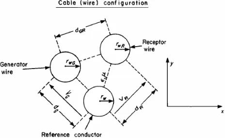
Adding a third conductor to the two-conductor system provides the possibility of generating interference [3–6] between the circuits attached to the ends of the line conductors resulting from crosstalk. In order to illustrate this important phenomenon, consider the three-conductor line shown in Fig. 1.
2.1. The Transmission Line Equations for Lossless Lines
In order to predict the crosstalk and understand the basic mechanism as well as the parameters affecting it, we will ignore these losses in formulating the multiconductor transmission-line equations in order to simplify their solution. Ignoring losses gives first-order and reasonably accurate predictions of the crosstalk. To obtain the MTL equations that we must solve in order to ∆z section as shown in Fig. 2. The generator and receptor circuits have per-unit-length mutual inductance lm between the two circuits. The line current
produce magnetic fluxes penetrating each loop formed by the conductor and the reference conductor, and these inductances represent the effect of those fluxes via Faraday’s law. The line voltages (between each conductor and the reference conductor) produced charges on the conductors that generate electric fields between each pair of conductors. This effect is represented by capacitances. The per-unit-length self-capacitances between the generator conductor and the reference conductor and between the receptor conductor and the reference conductor are represented by cG and cR, respectively. The
per-unit-length mutual capacitance between the generator and receptor conductors is represented by cm. In a ∆z section of the line the total
inductance or capacitance is the per-unit-length value multiplied by ∆z.
The MTL equations can again be determined from this per-unit-length equivalent circuit using circuit analysis principles and letting ∆→0, giving
∂VG(z, t)
∂z = −lG
∂IG(z, t)
∂t −lm
∂IR(z, t)
∂t (1a)
∂VR(z, t)
∂z = −lm
∂IG(z, t)
∂t −lR
∂IR(z, t)
∂t (1b)
and
∂IG(z, t)
∂z = −(lG+cm)
∂VG(z, t)
∂t −cm
∂VR(z, t)
∂t (1c)
∂IG(z, t)
∂z = −cm
∂VG(z, t)
∂t −(CR+cm)
∂VR(z, t)
∂t (1d)
An important observation can be made that aids greatly in the solution of these equations. Writing these equations in matrix form yields
∂
∂zV(z, t) = −L ∂
∂tI(z, t) (2a) ∂
∂zI(z, t) = −C ∂
∂tV(z, t) (2b) where
V(z, t) =
VG(z, t)
VR(z, t)
(3a)
I(z, t) =
IG(z, t)
IR(z, t)
(3b) And the per-unit-length parameter matrices are
L =
lG lm
lm lR
(4a)
C =
(cG+cm) −cm −cm (cR+cm)
The MTL equations in (1) are in the time domain. For single-frequency, sinusoidal steady-state excitation (phasor form) we simply replace time derivatives with jω, where ω = 2πf is the radian frequency of the source and f is its cyclic frequency. This method is
d
dzVˆ(z) = −jωLIˆ(z) (5a) d
dzIˆ(z) = −jωCVˆ(z) (5b)
3. THE PER-UNIT-LENGTH PARAMETERS
The configurations in Fig. 3 are considered to be lines immersed in a homogeneous medium [8]. The surrounding medium for the cases of three wires in Fig. 3 is logically considered to be free space with parameters ε0 and µ; that is, the wires are considered to be bare.
Dielectric insulations severely complicate the determination of the per-unit-length capacitances for wires, but do not affect the per-per-unit-length inductances since dielectrics have µ = µ0. For the lines in Fig. 3 we
will ignore the presence of dielectric insulations and consider the wires to be bare.
Figure 3. Wire type line cross sections whose reference conductors is a another wire.
If the surrounding medium is homogeneous, as for the lines in Fig. 3, the per-unit-length parameter matrices given in (4) have important, special relationships that parallel those found for two-conductor lines. In particular these relationships are
where the surrounding homogeneous medium is characterized by µ, and ε, and 12 is the 2×2 identity matrix:
12=
1 0 0 1
(7) Therefore we only need to determine one of the parameter matrices, since the other can be found form (6) as
C = µεL−1 = 1
v2L−
1 (8)
wherev= 1/√µεis the usual phase velocity for uniform plane waves, and is also the velocity of waves on the line for example, for the three-conductor line in a homogeneous medium we obtain from (8)
cG+cm −cm −cm cR+cm
= 1
v2(l
GlR−l2m)
lR −lm −lm lG
(9) Comparing the two sides, we obtain the per-unit-length capacitance parameters in terms of the per-unit-length inductance parameters as
cm =
lm
v2(l
GlR−l2m)
(10a) cG+cm =
lR
v2(l
GlR−l2m)
(10b) cR+cm =
lG
v2(l
GlR−l2m)
(10c)
4. THE INDUCTIVE-CAPACITIVE COUPLING APPROXIMATE MODEL
mutual inductance lm and mutual capacitance cm. In turn, these
induced currents and voltages in the receptor circuit will, as a second-order effect, induce currents and voltages back into the generator circuit. By assuming weak coupling, we mean that these voltages and currents induced in the generator circuit due to the currents and voltages that were induced in the receptor circuit may be ignored, that is, the induction of currents and voltages from one circuit to another is a one-way effect from the generator circuit to the receptor circuit. From the standpoint of the MTL equations in (1), the condition of weak coupling means that the equation for the generator circuit are approximated, by neglecting the mutual term as
∂VG(z, t)
∂z
+lG
∂IG(z, t)
∂t
= 0 (11a) ∂lG(z, t)
∂z
+ (cG+cm)
∂VG(z, t)
∂t
= 0 (11b) and the equations for the receptor circuit are unchanged
∂Vg(z,t)
∂z
+lg
∂lg(z, t)
∂t = −lm
∂lG(z,t)
∂t
(12a) ∂lG(z, t)
∂z
+ (cR+cm)
∂VR(z, t)
∂t
= Cm
∂lG(z,t)
∂t
(12b) The equations have also been rewritten by moving the self terms to the left-hand side in order to present them in the form of those for isolated two-conductor lines. Observe in the equations governing the current and voltage of the generator circuit (the circuit being driven by the source) in (11) we have omitted the mutual coupling terms lm∂IR(z,t)∂t and cm∂VR(z,t)∂t , which cause the back interaction of
inducing voltages and currents in the generator circuit due to currents and voltages and currents in the generator circuit due to currents and voltages in the receptor circuit. Thus we can solve for the voltage and current in the generator circuit,VG(z, t) andIG(z, t), as though it were
an isolated, two-conductor transmission line [11].
Once the voltage and current of this (isolated) generator circuit are obtained, we place induced sources due to these via the mutual inductance and mutual capacitance into the receptor circuit. The sources induced in the receptor circuit are represented by the terms on the right-hand-sides of the equations in (12).
−lm
∂IG(z, t)
cm
∂VG(z, t)
∂t (13b)
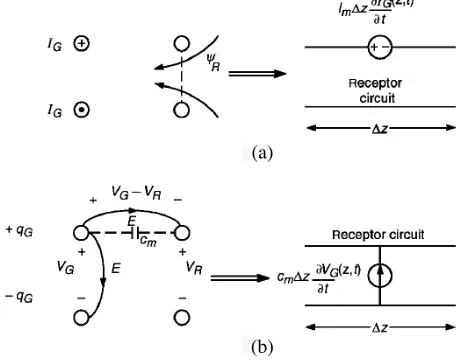
These sources induced in the receptor circuit are visualized as shown in Fig. 4.
(b) (a)
Figure 4. Explanation of the two components of crosstalk: (a) magnetic field or inductive coupling, (b) electric field or capacitive coupling.
Faraday’s law provides that a per-unit-length voltage will be induced in the receptor circuit that is due to the time rate of change of the magnetic flux penetrating the loop formed by the conductors of the receptor circuit. Hence two per-unit-length sources will be induced in the receptor circuit:
Vs1=lR
∂IR
∂t (14a)
and
Vs2 =lm
∂IG
∂t (14b)
Source VS1 is produced by the self-inductance of the receptor circuit.
Source VS2 is produced by the mutual inductance between the two
circuits and the current of the generator circuit. As a first-order model we will ignore the effect ofVS1. Hence we may represent the receptor
source is due to magnetic field coupling, it is referred to as inductive coupling. The total for a ∆zsection length will be the per-unit-length source multiplied by ∆z.
Current is the time rate-of-change of charge and hence per-unit-length current sources will be induced between the two conductors of the receptor circuit of
IS1 = (cR+cm)
∂VR
∂t (15a)
IS2 = −cm
∂VG
∂t (15b)
The first current source, IS1, in (16a) is simply the current source
induced by the receptor circuit self-capacitance. SourceIS2is produced
by the mutual capacitance between the two circuits. Again, as a first-order model we will ignore the effect of IS1. Hence we will represent
the receptor circuit with one source, IS2, as illustrated in Fig. 4(b).
Because this source is due to electric field coupling, it is referred to as capacitive coupling. Hence we will represent the receptor circuit by combining the two sources in (14b) and (15b) and lumping them together to represent the entire line with total mutual inductance and total mutual capacitance of Lm = lml and Cm = cml, respectively,
wherel is the total line length [12].
This is referred to as the inductive-capacitive coupling model. The crosstalk takes place via two distinct coupling mechanisms [13, 14], magnetic field coupling due to mutual inductance between the two circuits and electric field coupling due to mutual capacitance between the two circuits. There are two key assumptions in this model: (1) we assume weak coupling between the generator ands receptor circuits, that is, the coupling is a one-way effect from the generator circuit to the receptor circuit; and (2) the line is assumed to be electrically short at the frequency of the driving source in the generator circuit,Vsthat
is,lλ=v/f.
5. FREQUENCY DOMAIN INDUCTIVE CAPACITIVE COUPLING MODEL
Our first main interest is for driving sources in the generator circuit, Vs(t) in Fig. 1, that are single-frequency sinusoids; that is, we first
(a)
(b)
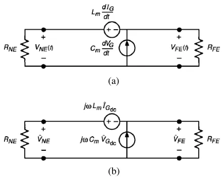
Figure 5. The simplified inductive-capacitive coupling crosstalk model: (a) time domain model, (b) frequency-domain model.
effectively the same as being effectively the same as though the driving source wasdc:
ˆ IGdc ∼=
1 Rs+RL
ˆ
VS (16a)
ˆ VGdc ∼=
RL
RS+RL
ˆ
VS (16b)
This is because we assume that the line is electrically short at the frequency of the driving source, i.e., l λ, where λ = v/f is a wavelength at the frequency f of the driving sinusoidal source, and hence the voltage and current do not vary appreciably in magnitude along the generator line. Hence they are virtually the same as those produced by a dc source. From this equivalent circuit we may determine the near-end and far-end phasor crosstalk voltages using superposition as [1]
ˆ VN E =
RN E
RN E+RF E
jωLmIˆGdc
inductive coupling
+ RN ERF E RN E+RF E
jωCmVˆGdc
capacitive coupling
(17a)
ˆ
VF E = −
RF E
RN E+RF E
jωLmIˆGdc
inductive coupling
+ RN ERF E RN E+RF E
jωCmVˆGdc
inductive coupling
and Lm = lml and Cm = cml are the total mutual inductance and
mutual capacitance of the line, respectively. ˆ
VN E =
RN E
RN E+RF E
jωLm
1 Rs+RL
inductive coupling
ˆ Vs+
RN ERF E
RN E+RF E
jωCm
RL
Rs+RL
ˆ Vs capacitive coupling (18a) ˆ
VF E =
RF E
RN E+RF E
jωLm
1 Rs+RL
inductive coupling
ˆ Vs+
RN ERF E
RN E+RF E
jωCm
RL
Rs+RL
ˆ Vs
capacitive coupling
(18b) The crosstalk can be viewed as a transfer function between the input
ˆ
Vs and the outputs ˆVN E and ˆVF E. These transfer functions can be
obtained by factoring out ˆVs and jω to give
ˆ VN E
ˆ Vs
= jω
RN E
RN E+RF E
Lm
Rs+RL
+
RN ERF E
RN E+RF E
RLCm
Rs+RL
(19a) ˆ
VF E
ˆ Vs
= jω
− RF E
RN E+RF E
Lm
Rs+RL
+
RN ERF E
RN E+RF E
RLCm
Rs+RL
(19b)
6. EXPERIMENTAL SETUP
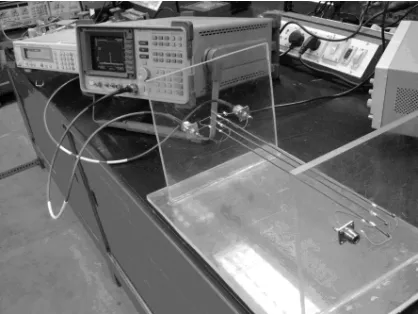
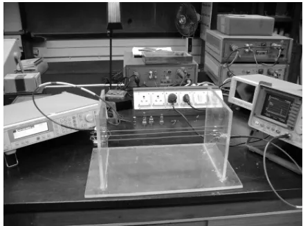
The three wire crosstalk model is shown in Fig. 6. The experiment setup for the measurements are shown in Fig. 7 and Fig. 8 respectively. In this setup the generator conductor and the reference conductor is terminated by 50 ohms at the far end side. Here the power received by the spectrum analyzer due to excitation voltage from the signal generator is studied over a wide frequency range from 100 MHz to 2 GHz.
Figure 6. Simple crosstalk model (Top view).
Figure 7. Experimental setup (Measuring near-end crosstalk).
at the input side or nearend side. Similarly for the measurement of the farend crosstalk voltage across the receptor conductor and generator conductor due to the presence of the third wire that is the reference conductor, we are using the same spectrum analyzer at the output side or farend side.
We are providing 10 dBm power from the signal generator to excite the crosstalk model. At the receiving side we are using the spectrum analyzer for practical measurement.
Figure 8. Experimental setup (Measuring far-end crosstalk).
L = 20 cm (Length of the wire), S = 1.3 cm (Distance between two adjacent wires) and Diameter of the wire = 3.5 mm
For simulating the whole model using CST (Computer Simulation Technology), we excited the three wire crosstalk model using discrete port [15]. For the measurement of the nearend and farend crosstalk voltage using CST, we are using 50 ohms lumped element, across which we are getting the nearend and farend voltage.
7. RESULTS AND ANALYSIS
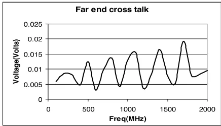
Figure 9 and Fig. 10 shows the simulated and measured results of nearend crosstalk voltage between the receptor wire and reference wire respectively when placed in an EM environment. Similarly Fig. 11 and Fig. 12 shows the simulated and measured results of farend crosstalk voltage between the receptor wire and reference wire respectively. The results show that both simulated and measured results are following the same pattern. The only small difference that we are getting is because of the whole experiment is performed in Microwave measurement laboratory, IIT Kharagpur where the environment is very much crowded. If the same experiment would have been performed in an anechoic chamber or an OAT site the results would have been quite better.
Near end Cross talk
0 0.05 0.1 0.15 0.2 0.25
100 600 1100 1600
Freq(MHz)
A
m
pl
it
ude
(V
ol
ts
)
Figure 9. Near-end crosstalk (CST simulated result).
Near End Crosstalk
0 0.005 0.01 0.015 0.02 0.025
0 500 1000 1500 2000
Freq(MHz)
V
o
lt
ag
e(
V
o
lt
s)
Figure 10. Near-end crosstalk (Measured result).
Far end cross talk
0 0.05 0.1 0.15 0.2 0.25
100 600 1100 1600
Freq(MHz)
A
m
pl
it
ude
(v
ol
ts
)
Far end cross talk
0 0.005 0.01 0.015 0.02 0.025
0 500 1000 1500 2000
Freq(MHz)
V
o
lt
ag
e(
V
o
lt
s)
Figure 12. Far-end crosstalk (Measured result).
simulated results are summarized as follows:
• The mismatch produced by the cables on transmit and receive side will contribute to the measurement error significantly.
• Though the scattering by other reflecting bodies in the vicinity are tried to minimize, can not be removed totally.
8. CONCLUSIONS
This paper presents the initial investigation of a simple crosstalk model by predicting the nearend and farend crosstalk voltage. in an EMI/EMC environment. The results from EMI/EMC stand point of view are very important for system design where implementation of multiconductor is necessary in any electronic system. Also the study can be extended for two wires with PEC as the reference conductor. The measurement of the nearend and farend crosstalk is an important part of the certification process needed before a device or system can be marked. This process has to be undertaken for all levels of devices from personal electronic devices up to large aircraft.
REFERENCES
1. Paul, C. R., Introduction to Electromagnetic Compatibility, 2nd edition, John Wiley & Sons Inc., New York, 1992.
2. Paul, C. R., Crosstalk, Handbook of Electromagnetic Compatibil-ity, Chapter 2, Part II, Academic Press, San Diego, CA, 1995. 3. Tripathi, R., R. Gangwar, and N. Singh, “Reduction of crosstalk
systems,” Progress In Electromagnetics Research, PIER 77, 367– 378, 2007.
4. Chen, H. and Y. Zhang, “A synthetic design of eliminating crosstalk within MTLS,” Progress In Electromagnetics Research, PIER 76, 211–221, 2007.
5. Kirawanich, P., J. R. Wilson, N. E. Islam, and S. J. Yakura, “Min-imizing crosstalks in unshielded twisted-pair cables by using elec-tromagnetic topology techniques,” Progress In Electromagnetics Research, PIER 63, 125–140, 2006.
6. Kirawanich, P., N. E. Islam, and S. J. Yakura, “An electromagnetic topology approach: Crosstalk characterizations of the unshielded twisted-pair cable,” Progress In Electromagnetics Research, PIER 58, 285–299, 2006.
7. Paul, C. R. and A. E. Feather, “Computation of the transmission-line inductance and capacitance matrices from the generalized capacitance matrix,”IEEE Trans. Electromagn. Compat., Vol. 18, No. 4, 175–183, Nov. 1976.
8. Paul, C. R., “Solution of the transmission line equations for three-conductor lines in homogeneous media,” IEEE Trans. Electromagn. Compat., Vol. 20, 216–222, 1978.
9. Bernardi, P., R. Cicchetti, G. Pelosi, A. Reatti, S. Selleri, and M. Tatini, “An equivalent circuit for EMI prediction in printed circuit boards featuring a straight-to-bent microstrip line coupling,”Progress In Electromagnetics Research B, Vol. 5, 107– 118, 2008.
10. Paul, C. R., “Solution of the transmission-line equations under the weak-coupling assumption,” IEEE Trans. Electromagn. Compat., Vol. 44, No. 3, 413–424, Aug. 2002.
11. Chai, C., B. K. Chung, and H. T. Chuah, “Simple time-domain expressions for prediction of crosstalk on coupled microstrip lines,”
Progress In Electromagnetics Research, PIER 39, 147–175, 2003. 12. Paul, C. R., “On the superposition of inductive and capacitive
coupling in crosstalk prediction models,”IEEE Trans. Electromag. Compat., Vol. 24, 335–343, 1982.
13. Xiao, F. and Y. Kami, “Modeling and analysis of crosstalk between differential lines in high-speed interconnects,” PIERS Online, Vol. 3, No. 8, 1293–1297, 2007.
14. Xiao, F., R. Hashimoto, K. Murano, and Y. Kami, “Analysis of crosstalk between single-ended and differential lines,” PIERS Online, Vol. 3, No. 1, 16–20, 2007.