Multivariate statistical methods to determine changes in botanical composition Vegetation.

(1)

Multivariate Statistical Methods to Deter-

mine Changes in Botanical Composition

WALTER W. STROUP AND J. STUBBENDIECK

Abstract

Confusion exists over the proper statistical methodology to use in analyzing the effect of treatments on changes in botanical com- position over time. A rationale for using multivariate statistics is presented. Basic considerations involved in the use and interpreta- tion of multivariate statistics specifically appropriate to the botani- cal composition problem are given. An example of how such an analysis can be performed using a common statistical computing package (SAS) is demonstrated.

Change in botanical composition over time is one way of meas- uring the effect of applied treatments on vegetation. The point method was developed by Levy and Madden (1933) and has been commonly used to determine botanical composition based on the proportion of the ground or area occupied by plant bases or covered by foliar portions of the vegetation (Brown 1954, Cain and de Castro 1959, Greig-Smith 1964, Kershaw 1975, Tothill 1978). These point data, along with cover data collected by other tech- niques, have been analyzed by various methods, and some confusion generally exists as to the proper method of evaluation of the effect of “v” different treatments (v 2 2) on changes in botanical composition over time. The researcher needs to know how such an experiment should be designed and analyzed so that this evaluation can be made. Analysis of data collected from an experiment of this type is complicated by the fact that the response variables of interest (i.e. counts or percentages of the various species) are highly correlated.

The objectives of this paper are: (I) to suggest an experimental design which will provide data addressing the above research question without ambiguity, (2) to make the range scientist aware of the statistical problems inherent in analyzing sets of correlated response variables, and (3) to suggest procedures which should be utilized to correctly yet clearly analyze these data. These procedures require use of statistical computing packages. While several good packages exist, examples will be given for implementation using the Statistical Analysis System (SAS) (Barr et al. 1979) probably the most widely available statistical package at agricultu- ral experiment stations.

Statistical Problems Inherent in Analyzing Botanical Com-

position Data

Suppose an experiment is conducted in which v treatments (v 2 2) are applied to plots within each of r blocks (r2 2). At each oft times (t 1 2) the percent composition for each of s plant species is observed for each plot. The objective is to decide whether the changes in species composition are affected by the treatments. How shall a question be addressed?

To answer this question, it is necessary to recognize the experimental design implied by the procedure described above. This experiment can be viewed as a split-block, with treatment as the whole-plot effect and time as the split-block effect. The basic appioach to the analysis of this type of experiment, the method

Authors are assistant professor of biometry and professor of agronomy (range man- agement), University of Nebraska, Lincoln 68583.

This report is published as Paper Number6619, Journal Series, Nebraska Agricul- tural Experiment Station.

206

presented in most introductory classes in experimental design, is univariate analysis of variance (ANOVA). This analysis is appropriate if the objective is to evaluate only one response variable or a set of uncorrelated response variables one at a time. For example, suppose the change in only one species is of interest: all other species are simply ignored. Granted, this is unrealistic but it is important to understand the basics before elaborating the problem.

In the one variable case, the split-block experiment described above gives rise to the following ANOVA.

Source of Variation df

Block r-l

Treatment V-l

error a Time

if;; (v-l)

error b (r-l) (t-1)

Time X Treatment (v-l)(t-I) error c (v-l)(t-I)(r-I)

The research question posed by the experimenter can be phrased in terms of the statistical hypothesis H,: no time X treatment interaction exists versus HA: a time X treatment interaction does exist. That is, H, corresponds to stating that the changes over time in the percent of the species are identical for all treatments; HA corresponds to stating that these changes over time are different for at least one of the treatments. The mechanics of this analysis can be found in Steel and Torrie (1980).

A more complex situation arises, however, when the

experimenter is interested in the total relative species composition of the plot. Let yijkl denote the proportion of the lth species at the

kth time period for the jth treatment in the ith block. Then d yijkl ‘I=1 = 1; that is, for a given plot at a given time, the sum of the proportions for each species must be one. From a statistical analysis point of view, this is a critical point: within a given plot at a particular time the observations on the various species are nega- tively correlated. That is, an increase in the YAM for one of the “s”

species must necessarily be accompanied by a decrease in the yijkl for one or more of the other species being studied. Therefore, the collection of proportions of each species must be analyzed taking this negative correlation structure into account. The proper way to do this statistically is to utilize multivariate statistical methods, specificially, multivariate analysis of variance (MANOVA).

The similarities and distinctions between the appropriate linear models and hypotheses tested for the usual univariate ANOVA and MANOVA in the context of the botanical composition experiment are reviewed. In addition, the range scientist will be aquainted with the assumptions underlying thedata which must be satisfied to validly apply MANOVA to such data. Finally, the method for programming such analyses using the Statistical Anal- ysis System (SAS) will be demonstrated. No attempt will be made to present a detailed account of MANOVA theory. Readers interested in pursuing this topic are encouraged to read further in such multivariate textbooks as Morrison (1976).

(2)

Hypotheses Tested and Assumptions Involved in MAN- OVA for Botanical Composition Problem

To understand the hypotheses tested and the assumptions underlying MANOVA for the species composition problem, hypotheses and assumptions involved for the univariate ANOVA case must be understood. Consider, as an example, data from an experiment conducted as described above with the number of species observed s = 1. Let yijk denote the count or percent for that species for the ith block, jth treatment, and kth time period. The linear model for this experiment can be represented by the following equation:

yik = /J -t bl -t Vj ‘t (bvh -t tk t (bt)ik ‘t (vt)jk -t (bVt)ijk (1)

where p = the overall mean

bi = the effect of the ith block, i=1,2 ,..., r

Y = the effect of the jth treatment, j=1,2...,v

(bv)ii = random error associated with the ijth block treatment combination (error a)

= the effect of the kth period, k= ,2 ,..., t

;&k = random error associated with the ikth block-time combination (error b)

(vt)jk = interaction effect for the jkth time-treatment combination

(bVt)ijk = random error for the ijkth block-treatment-time combination (error c).

The null hypothesis of no interaction between treatments and time periods can be stated in terms of (1) as H: (vt)jk = 0 for all j=1,2 ,..., v, k=1,2 ,...,t. This hypothesis can be validly tested using ANOVA provided each of the error c terms (bvt)ijk has a normal distribution with constant variance, ~3, for each block-treatment- time combination. Note that species counts for this example would actually follow a binomial distribution, but ifthe number of points per plot is large the counts will approximate a normal distribution. It is important that this consideration be kept in mind when designing and conducting the experiment. The equality of the variance of the error c terms is a more severe requirement and should be check using an appropriate procedure such as Bartlett’s * test (Steel and Torrie 1980). If this requirement is not satisfied, ANOVA on the percents should not be performed (see below).

Now consider an experiment using the same design as above but for which s > 1 species are observed. Let yd~. denote the count or percentage on the ijk-tk block-treatment-time combination for the lth species. Analogousto the univariate model (l), the multivariate linear model can be expressed as:

yijkl = /.&I .fbil -t Vii -t (bvki ‘f tkl -t (btku t (Vt)jkl -t (bVt)iiki (2) where the terms on the right-hand side of the equation correspond to the effects for model (1) for the lth species, 1=1,2,...,s. Then the hypothesis of no interaction for model (2) can be expressed as H,: (vt)jkl = 0 for every treatment combination, i.e. (3)

the changes over time for each species are identical for every treatment.

The hypothesis given in (3) can be validly tested using MAN- OVA if the following assumptions hold for the destribution of the (bvt)ijM or error c, terms.

1) The error c terms must be normally distributed. As in the univariate case, satisfying this condition requires a large number of points per plot. Additionally, species with very small counts occurring for a large number of block-treatment- time combinations should either be left out of the analysis or grouped together into classes of related species. NOTE: To insure that the statistics used to test the hypothesis given in (3) can be calculated, the number of species or species classes should be less than the number of treatments.

2) Let ozju denote the variance of the error c term for the jkl-th combination, and let Ujkl’l denote the covariance of the error c term for two species 1 and l’, where 1 # 1’. The error structure among the error c terms for the s species for the jkth

treatment-time combination can be represented by the following matrix:

I

Ujk12 UjklZ- - - Uj,kls

l.

. .

Ujkb-1)s

. Ujks2

The requirement for the error structure for valid application of MANOVA is that the matrices cjk must be eqUd for each treatment-time combination. This assumption corresponds to the requirements of equal variances in univariate ANOVA. If the data show gross deviation from this assumption alternative methods of analysis should be considered such as the alternative presented below in the section “Some Suggestions for Analyzing Botanical

Composition Experiments when the Assumptions of MANOVA

are Violated.”

In univariate ANOVA, the hypothesis of no interaction istested by calculating the Sum of Squares for Treatment X Time and the Sum of Squares for error c and then ‘calculating the ratio

F= SS(treatment X time)/@-l)(t-1) SS(error c)/(r-l)(v-l)(t-I)

and comparing F to a table value of the F-distribution with (v-l)(t- 1) and (r-l)(v-l)(t-1) degrees of freedom at an o-level correspond- ing the experimenter’s willingness to risk committing a type I error.

The situation becomes more complex when testing the multivariate hypothesis of no interaction given by (3). Rather than using a single sum of squares to measure variability attributable to time- by-treatment interaction for a single response variable, the multivariate procedure utilizes a matrix consisting of sum of squares terms measuring treatment-by-time effects for each of the correlated response variables and sum of products terms to account for the covariance among treatment-by-time effects of the various species. In place of a single sum of squares for error, a matrix is used which is similar to the above matrix except time-by-treatment terms are replaced by error terms. These matrices are known in the literature as the hypothesis, or H, matrix, and the error, or E, matrix respectively. The mechanics of calculating these matrices is beyond the scope of this paper; readers interested in pursuing the subject are referred to Morrison (1976).

The matrices H and E cannot be divided to produce a single test statistic as in the case of a univariate F-test. However, there are methods for comparing H and E, that is, testing the multivariate hypothesis of no interaction, which are commonly accepted multivariate procedures. Four which are computed by SAS are (1) the Hotelling-Lawley trace, (2) Pillai’s trace, (3) Wilk’s Lamda, and (4) Roy’s Maximum Root Criteria. There is no general agreement among statisticians which of these statistics is “best.”

For the purposes of the range scientist it is sufficient to now that the H and E matrices and their associated test statistics will be calculated by SAS. Any of the test statistics would be considered acceptable for publication. The levels of significance associated with the comparison of H and E corresponds to the level of significance for the test of the hypothesis of no interaction. Addi- tionally, an important practical consideration is that at most s-l species or species group counts should be included in a single MANOVA run. For matrix algebra considerations beyond the

8

scope of this paper, the fact that c yuki = 1, i.e. y ijks is determined I=1

by yjkl,...,yijL, @-I, makes it algebraically impossible fo’r any of the test statistics to be calculated. However, if a time-by-treatment interaction is detected for s-l species, it follows that it must apply as well to the sth species, because of this dependency. If the hypothesis of no interaction is rejected, the biological interpretation is that changes in the counts over time are affected by the treatments for at

(3)

least one species or species group. Specific hypotheses concerning which species are involved in the interaction and the components of that interaction can be pursued using multivariate contrasts. The mechanics of these contrasts involve considerable,matrix algebra manipulation and are beyond the scope of this paper. How- ever, a simple method for the range scientist to visualize the nature of the interaction is to obtain a three-dimensional plot of the relationship between time and treatment for each species, (See

appendix). /

Suggestions for Analyzing Botanical Composition Experi-

ments When Assumptions of MANOVA Are Violated

It is important to emphasize that the test of the hypothesis of no interaction using MANOVA is valid only if the assumptions given in section IV are satisfied, i.e., that the counts are approximately normally distributed and, more importantly, that the & matrices are approximately equal for each treatment-time combination.

The assumption of approximate normality can best be dealt with by keeping the central limit theorem firmly in mind while designing the experiment. Specifically, the experimenter should plan to read a relatively large number of points per plot per occasion and plan on grouping together related species in situations where counts for the individual species are small or zero. While no absolute rule exists for exactly how many points should be read, with a lo-point frame, the authors have had good success using several hundred points per plot in short and midgrass vegetation types and feel that less than this number would present the experimenter with problems in determining significant treatment differences.

The assumption of equal Ct matrices is not as easily handled. To understand this, consider the following argument. Strictly speak- ing, the counts of the various species for a given plot on a given occasion are distributed according to a multinomial distribution. That is, let pijkl = the probability of sampling the Ith species in the ijth plot on the kth occasion, let N be the number of points per plot per occasion, and, as before, you be the count for the Ith species. Note that

* *

cpijlrl= 1 and ,$tr=N I=1

Then probability of a particular configuration of counts Yijkl, yij- tiv..Yijkss is given by

N

yijkl!j'iikS!...&jb!

Moreover, the variance of a particular count, denoted U’ijkt, is

U*iju = Npijkl(I-fikI)

and the covariance, denoted by a~u I, is

(4)

Oijkl I = -NPtiu ~II (5)

As mentioned earlier, if the bjkl are not too close to 0 and if N is large, the multinomial is approximated by a multivariate normal distribution. But, if the pijkl change dramatically for the various treatments or times, then o’ikl and Oiikfl will be altered and hence the Ct matrices will not be equal. This fact follows directly from formulae (4) and (5) and thus cannot be addressed by the experimental design.

One approach to this problem involves a variance-covariance stabilizing transformation appropriate for multinomial data. A particularly useful transformation is

&iu = arcsin (dx

Let C’,* be the variance-covariance matrix of the Xijkr, which will have the same form as C,,t except the transformed variables are used in the calculation. If the C’- are shown to be approximately equal then, MANOVA can be calculated using the x+t.

Unfortunately, variance stabilizing transformations are not always successful. A common situation in this type of experiment arises when differences in the C, are due primarily to difference in

the yrju over time. If the data suggest that the Ct are different, an

appropriate way of looking at the data is to use the following model:

yiikl = ,&I -t hiU t tjkl -t %jkl

where /lkl = overall mean for time k, species 1. b&l = ith block effect for time k, species 1.

tjkl = jth treatment.effect for time k, species 1.

eijkl = random error for time k, species 1.

In essence, one is looking at the species by time counts as a set of correlated responses for each plot. The statistical theory and methods for analyzing problems similiar to the species composition problem are described in full by Grizzle and Allen (1969). Specific SAS programming considerations are given by Courtright (1978). An elaboration of this technique specific to botanical composition problems is given by Stroup (1982).

A final alternative approach to the problem is to look at the counts as categorical data. That is, the response variable in this experiment for each hit within a plot is actually a category, i.e. a species. Grizzle et al. (1969) presented a method of analyzing categorical data from a linear models point of view. The programming for this approach can also be accomplished in SAS, using the procedure entitled FUNCAT. A drawback to this approach is that if any of the )‘ijkl= 0, a small positive number must be substituted in its place. The authors warn that the effects of this on the validity of levels of significance for the hypotheses tested, specifically in this case, the hypothesis of no time X treatment interaction, are not known. Therefore, if this approach is used, it is important that species be grouped so that no zero counts occur in the data. Recall, however, that rare counts also present theoretical problems in MANOVA. The advantages and disadvantages of FUNCAT versus MANOVA for this type of data are not well understood by statisticians at this time and require further study.

Conclusion

When analyzing data from a botanical composition experiment, correlation among the various species counts is inevitable. Univar- iate analysis one species at a time does not account for correlation among species whereas a multivariate approach does. For this reason, the multivariate procedure is recommended. The principal advantage to the experimenter is that by exploiting the informa- tion about correlations, the power of the test for interaction, that is, the likelihood of detecting an interaction if it exists, is increased. Several multivariate approaches exist. MANOVA is generally applicable, its statistical properties are well understood, and it is

relatively easy to program using SAS. Among the newer

approaches, a linear model approach to the analysis of categorical data, which can be programmed in SAS using the FUNCAT procedure, appears to be very promising. However, the statistical properties of this procedure need to be better understood before it

can be generally recommended as an analytic tool.

Literature Cited

Barr, A J., J.H. Goodnight, J.R. SalI, W.H. Blair, and D.M. Chilk. 1979. SAS Users Guide. SAS Institute, Raleigh, North Carolina.

Brown, D. 1954. Methods of surveying and measuring vegetation. Com- monwealth Bur. of Pastures and Field Crops. Hurley, Berkshire, Eng- land. Bull. 42.

Cain, S.A., and GM. deCastro. 1959. Manual of vegetation analysis. Harper, N.Y.

Courtwright, J.A. 1978. Repeated Measures in SAS. Proceedings of the Third Annual SAS Users Group International Conference. SAS Insti- tute, Raleigh, NC.

Greig-Smith, P. 1964. Quantitative plant ecology. Butterworths. London. Grizzle, J.E., and D.M. Alien. 1969. Analysis of growth and dose response

curves. p 357-381. Biometrics. 25.

Grizzle. J.E.. C.F. Starmer. and G.G. Koch. 1969. Analysis of categorical

databy linear models. p: 489-W. Biometrics 25. _ -

Kershaw, A. 1975. Quantitative and dynamic plant ecology. Amer. Elsevier Publ. Co. N.Y.

Levy, E.B., and E.A. Madden. 1933. The point method of pasture analysis. New Zealand J. Agr. 34145-164.

(4)

MorrIson, D.F. 1976. Multivariate statistic methods. McGraw-Hill. New York.

Steel, R&D., and J.H. Torrie. 1980. Principles and procedures of statistics-a biometrical approach. 2nd ed. McGraw-Hill. New York. Stroup, W.W. 1982. Use of SAS to Analyze Experiments with Multivariate Response Variable and Autocorrelated Errors. Proceedings of the Sev- enth Annual SAS Users Group International Conference. SAS Institute, Gary, N.C.

Totbill, J.C. 1978. Measuring botanical composition. p. 22-67. In: &asure- ment of grassland vegetation and animal production. Ed. L.

l

tMannetje. Commonwealth Bur. Pastures and Field Crops. Hurley, Berkshire, B.M. 52.

Appendix

Example of Use of SAS-MANOVA

Consider an experiment in which the effects of five herbicides on rangeland containing an undesirable shrub are compared. Four blocks containing five plots each are used. To each block, the five herbicides are assigned at random for application, one herbicide to a plot. Basal cover data are collected using the point method during the first growing season after application. These data are subse- quently converted to botanical composition. Let the data for this season correspond to time 1. This procedure is repeated during the next growing season (time 2) using the same assignment of herbicides to plots and again during times 3 and 4. Basal cover data are grouped into these categories: species group 1, species group 2, . . . . species group 4. The four species groups are then analyzed using MANOVA.

Using SAS, MANOVA is programmed by the following statements:

DATA A,

INPUT BLK TRT TIME SP_l SP-2 . . . SP-4

CARDS:

data-one card per block-treatment-year combination. NOTE: each card will consist, in order, of an identification number for the block, followed by a space, followed by treatment identification number, space, time (year) identification,

space, frequencies or percentages for each species, each separ- ated by a space. After all data cards are placed in the program,

then the cards for MANOVA are specified: PROC GLM; CLASSES BLK TRT TIME;

MODEL SP-I - SP-4 = BLK TRT BLK*TRT

TIME BLK*TIME TRI*TIME/NOUNI; MANOVA H = TRT*TIME/PRINTE;

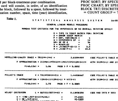
The NOUN1 option suppresses univariate analyses of variance which would otherwise be printed for each species. The PRINTE option causes correlations among the species groups to be printed. While the table of correlations is self-explanatory, the MANOVA output requires some explanation. The output is given in Table 1.

The important result is the PROB > F value under Wilk’s Criterion. The value .0050 indicates that the hypothesis of no time X treatment interaction is to be rejected forany alpha levelexceed- ing .0050. In other words, for at least one species, there is a difference among the treatments in botanical composition over time, aside from a 0.5% chance of type I error.

To visualize this interaction, PROC CHART (a univariate approach) is used to examine changes in botanical composition over time for each treatment. One such chart is printed for each species. The SAS program for obtaining these charts is as follows. The statements assume the charts will be programmed immediately after MANOVA in the same run as MANOVA.

DATA B; SET A;

SPECIES = 1; COUNT = SP-I; OUTPUT;

SPECIES = 4; COUNT = SP-4; OUTPUT; DROP SP-I - SP-4;

PROC SORT; BY SPECIES; PROC CHART; BY SPECIES;

BLOCK TRT/ DISCRETE TYPE = MEAN SUMVAR = COUNT GROUP = TIME;

Table 1. _SlATISllCAL _ANAl.vsIs _SVSlCI(

lb105 IWXSOAV. MAY Zvr 19.2 ,

GENEXAL LINEAl MODELS PAOCEOUAE

MNOVA TESr CRIvEfIIA FOX TrY HlPOlMESlS OF NO OVERALL vXv*lll#E EFFECI

M l WCC IV SSCCP NATXIX FOX; lRl*lfllE E l EAROX SSLCP UXRIX

P l WC. VAAIAOLES . 6

0 l HVPOvnESIS OF -

NE= OF OF E . ::

5 - MIllO*Ol . A

I4 l .slAeslP-o1-1~ -

N . .ItNE-P-11 = 1:::

---~~~~~---~~~~~~~~~~~~~~~~~~~~~~~~~~~~~~~~~~~~~~~~~~~~~~~________

MOTELLIWG-LAnLEv 1xACE I TIIEW-IWI . 2.3359,959 (SEE PILLAt’S IAOLE 931

F APPRUxl~AllON = 2~S~~1~9tR~E9~-l*rll~S9S*~2x*S*llI YITH St2M*S+ll AN0 2lS*N*ll DF

Fl4A112bl = 1. Xb PLOD > F = 0.0032

----~_~~__~___~___~_____~____~~_~_~_~~_~_____~_______~___~____________~___~_~~~~_~_~____~_____

PILLAl’S IMCE v - IXL~INV~~*E~ - 1 .W939bbV #SEE PILLAl’S TAOLE I21

F APPRUXtIulION = (2N6~1l1l21(6+1~ 9 VItS-VI YITM St2lWS+ll AN0 SIZN*S*lt OF

Fik3.lIII 0 1.10 PRO0 > F = 0.0095

______~__~_~~_~_~___~_~____~~~~~~I__~___~___________~____I_______________~~~~~~~~~~______~

Yl LXS’ CRI vER10N L = OE~lE)/OEllM~El . 0.1395025. (SEE RAO 1973 P 5551

W - -~NE-.5IP-O+II~*LN~L~ I 17.3021

u - te-.5lP-G7*ll I 39.5900

2 = SOIIll~P*y~P-*~llP*P*Q*P-5l - 3.9521

9 = (PW-2114 I 11.5090

F APPIOXI~UION = IU92-2ol/~P*a~*~l-L**l/zl/L**l~2 YIlM P*P AN0 WI-29 OF

F(49tl29l = 1.30 PROI > F = 0.0050

____~-_~_~__~_--_~_~~~~~~~_~-_-___~________~__~_______________~__~~~~~~~~__~_~_____~__~

101’5 #AXtWM A001 ClllIEAION . l&3*31 7bA lSEE US VOL 31 l b25)

FIRS1 CANONlCAL VYIAIYE VlELOf AN F UPPER BOUWD

Fll2,3bl - l .30 (UPPEX UJUNOJ

_~_________~____-________~______~~~~~~~~~~~~~~~~~~-_-________-__~~I~_____-_______~

(5)

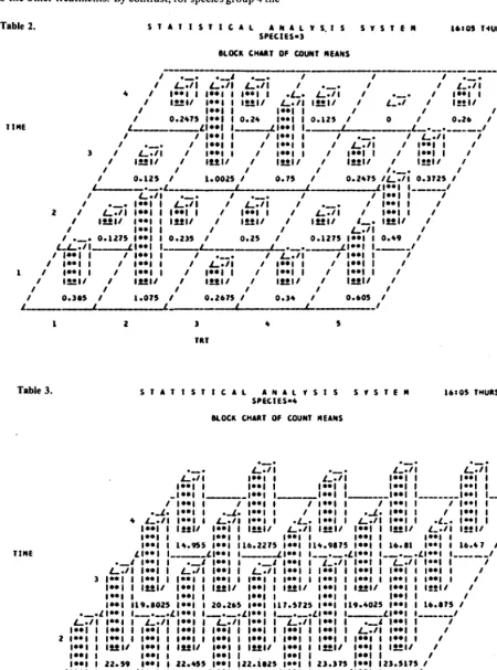
As examples of the output, consider the block charts for species 3 and 4. The output is given in Tables 2 and 3.

Notice that for species group 3 there are pronounced differences in the development of botanical composition based on basal cover over time, particularly for treatment 2 and for treatment 5 compared to the other treatments. By contrast, for species group 4 the

trends in botanical composition over time are virtually identical for each treatment. In this fashion the effect of the treatments among species can be described qualitatively. As mentioned in the text of this article, this can be further pursued quantitatively using contrast methods discussed in detail in Morrison (1976).

TIME

SIAIISTICAL ANALVS.IS 5VSlCM IbIOS IWRSOAV. MAV Zlr. 1992 11

SPECIES=3

ROCK CWAT OF COUNT MEANS

___---_ -- ---_____---__-__

I’

i7i

iZiS:

iTii

I

If

I

I.01 I I*+1 I I**1 I .Li. iTii

I r:Zi f'

4 I I**1 I ,

If 1~1, I**1 I I*11 L./I IzLlf I/ L:z' // I%11

I

I**1 I I**1 I I / I

/ 0.24?5 I**I I 0.24 I**1 I 0.125 I 0 0.2b I

_m- Ll**l 1_,11**1 I

I

0.2475 /;si 0.3725 I'

2 Ii

//

. 0.1275 I**1 i 0.235 I 0.25 I 0.127) IGI I 0.49 I

_-L-

/ I+*1 I I I**1 I I .__.

I I**1 I I I**1 I

I**I I ,' &'l I

I I**1 I I I**1 I I

1 / IL.1 I I I..1 I , I**1 I

/ lfzll

I, IMII /, 1**1/ I lfi.1,

l~l, ,,

I,

,

0.305 , 1.075 , 0.2b75 /' 0.34 , O.bOS I

Table 3.

1 2 3 4 5

1117

TINE

SlA71SlICAL ANALVSIS SVSTEM lb:05 TWASDAV, IlAY 27, 1992 12

SPECIES=4

MOCK CIiAR7 OF COUNT MEANS

iT?i iZii

rlrii iTii

I**1 I LZi I**1 I I..1 I

I**1 I I**1 I I**1 I I**1 I

_I**1 I ._I.'1 I -- ;::I 1 _-__-l**l I,. .I**1 I _I___

I I+*1 I / I**1 I I I*+1 I I I**1 I I I**1 I /

._L. I*'1 I ._f. I**1 I I I**1 I ._f. I**1 I I 1.01 I I

4 L./I I..1 I L./I I..1 I

I I 12*1/ I*+1 i 1221'

.L_. I**1 I L./I I**1 I

LQiI lrl/ I**1 I Lfii I*.1 I

I**1 I"11 l2?l/ f'

I**1 I I**1 I I**1 I I**1 I ,..I ,--. . 1 ,

I**1 I 14.955 I**1 116.2275 I**I 114.9975 l**l I lb.8 I ID.1 I lb.47 /’

Ll**l I _a-_ LWI I __/I**I I ._.LI..l I__._.LI**l I______/

._I 1.91 I .,I 1.01 1 ._I Ieel I-i-./l l*+I I , .,I I**1 1 ,

L./I I**1 I L./l I**1 I L./I I*+1 I I**1 I I**1 i lisi i i**i i 1~

3 I**1 I 1.01 I I**1 1 I**1 I IGI I I.'1 I I**1 I I**1 I I**1 I I**1 I ,

I**1 I Ial/ I**1 I 11111 I+*1 I l*I/ I**1 I Ifi I**1 I ILtl,

I**1 I I..1 I I**1 I I**1 I I**1 I I,

I**I 119.8025 I**1 I 20.265 I**1 117.5725 I**I 119.4025 I**I I lb.875 I

._.fl**l I _-.__. Ll**l I _._.LI**l I -.__. LI**l I__ LI..l I _---/

L./I I**1 I L./l I**1 I L./l I**1 I L./I 1.01 I .__1 I.'1 I I

I**1 I I**1 I I**1 I I**1 I I**1 I I**1 I I*+1 I I**1 I L./l I**1 I I

2 I**1 I I.01 I IO.1 I I**1 I I**1 I I**1 I I**1 I I**1 I I..I I I..1 I

I**1 I la!l, I**1 I ls$l/ I**1 I 11111 I+*1 I IlLI/ I**1 I IEI, ,'

I**1 I I*+1 I I**1 I I**1 I

I**I I 22.59 I**l I 22.4S5 I**1 l22.iO25 1::; f 23.375 I**1 I23.517S I'

LI..l 111**1 1,r1*+1 1.L1r.1 I__ LI.'l I

I I*+1 I I I**1 I I WI I I l..I I I I*.1 I -+

I I**1 I / I**1 I / I**1 I I I**1 I I I**1 I 1

I,

I**1 I / I.'I I

ISI/ /'

I**1 I I 1.01 I , I..I I

lP.~l, I,

Is!2l/ I 1111, , I*11 ,

, ,

23.675 I 24.495 /'

I/--_

23.9925 , 23.375 Ii

I , 22.w25,/,

1 2 3 4 5

IIT